Computing Active Power Losses Using a Mathematical Model of a Regulated Street Luminaire

Abstract

Before the use of regulated street luminaires with variable power and luminous flux, computations were performed using constant values for their electrical and photometric parameters. At present, where such lighting is in use, it is no longer possible to base calculations on such assumptions. Computations of energy and power losses, for example, need to be performed for all dimming levels and based on the applied regulation algorithm. Based on measurements carried out on regulated luminaires, it was found that certain electrical parameters have a nonlinear dependence on the dimming level. Electrical parameters were also observed to depend on the value of the supply voltage. The results of the measurements are presented in this article. Failure to take account of power losses in computations of the energy efficiency of street lighting in accordance with the applicable EN 13201 standard causes values of energy efficiency indicators to be overstated. Power loss computations are presented in this article for a sample street lighting system with regulated luminaires, for the whole range of dimming levels and additionally for fluctuations of ±10% in the supply voltage. In addition, a mathematical model of a regulated luminaire is constructed with the use of regression methods, and a practical application of that model is described.

1. Introduction

European Union recommendations concerning improvement in energy efficiency cover 25 areas of action under seven priorities. One of these priorities is lighting, the others being buildings, equipment, transport, industry, power plants, and interdepartmental issues [1,2]. Lighting is an area where energy efficiency can be improved by means of a relatively small financial expenditure [1,3,4,5,6]. It is achieved most often by replacing light sources or by modernising or replacing luminaires. The use (although not exclusively) of modern light sources or luminaires based on LED technology makes possible the use of regulation systems [6,7,8]. The simplest regulation system, and the kind most commonly used in practice, is based on an illumination schedule implemented in a luminaire controller [8]. These schedules may be identical for all days and seasons, or may include seasonal variation. The illumination schedule determines the degree of reduction of power and luminous flux at particular times in the evening and night. The PN-EN 13201 standard [9] permits changes in the lighting class of a road at times of lower traffic volume. A change of lighting class allows a reduction of the luminous flux of the luminaire, which is equivalent to a reduction of its power. The power reduction should not cause the illumination conditions to fall below those laid down in PN-EN 13201 [9]. Often in practice, during the modernisation of street lighting, insufficient care is taken to ensure that the requirements of PN-EN 13201 [9] are satisfied at reduced levels of power and illumination. Advanced (intelligent) systems of street lighting control enable the regulation of individual luminaires and of whole systems. They also enable diagnostics of luminaires and monitoring of electricity consumption [10].

Section 5 of the standard [9] defines indicators for evaluating the energy efficiency of street lighting, taking account of the consumption of energy when adequate street lighting parameters are maintained. One of the indicators for evaluating the energy efficiency of a lighting system is the power density index (PDI), D_P. This represents the electrical power needed to provide an adequate level of road illumination. It is computed by dividing the active power P of the lighting system by the sum, over a set of considered horizontal planes, of the product of the average illuminance on a plane E_i and the area of the plane A_i:

$$D_P=P/{\displaystyle \sum _{i=1}^n\left(E_i·A_i\right)},$$

(1)

Another indicator is the annual energy consumption index (AECI), D_E:

$$D_E={\displaystyle \sum _{j=1}^m\left(P_j·t_j\right)}/A$$

(2)

This is computed as the sum, over periods of operation of the system during the year, of the product of the power of the lighting system in a period (P_j) and the duration of the period (t_j), divided by the area illuminated (A). The power of the lighting system P (P_j) is computed as the sum of the powers of the light sources and the total power of devices of the system necessary for its proper functioning. The value of the power of the system affects both of the above-mentioned indicators of street lighting efficiency. The standard does not specify whether power losses are to be considered in the computations, although in precise computations they should be taken into account. It would therefore appear important to estimate how the accuracy of computations of these indicators is affected by the decision to neglect or to consider power losses in the street lighting system.

Analysis of the energy efficiency of street lighting in accordance with the PN-EN 13201 standard [9] requires knowledge of the mean illuminance on the road, the size of the area illuminated, and the power of the lighting system being considered. Computations are usually performed based on the rated powers of the luminaires, neglecting power losses in the system components. An increase in power losses will lead to an increase in consumption of active power and in electricity charges. Failure to take this issue into account during an energy audit may lead to discrepancies between the results of theoretical computations and the actual consumption of active power. The losses of active power in a street lighting system depend on the complexity of the network, the number of circuits and the numbers of luminaires in each circuit, the power supply and control devices used, the level of reactive power in the network, etc. In making an economic analysis of the losses, it is possible to describe in detail the impact of just one component of the power supply system, which may be significant in this context [11,12].

Active power losses in lighting networks can be reduced by using devices with regulated parameters [13] and by limiting the reactive power in those networks [14]. During laboratory tests of LED street luminaires with regulated power, the authors have observed that the displacement power factor and the THD (Total Harmonic Distortion) of the current depend greatly on the dimming level. In a real supply network, the voltage very often deviates from the rated value. The EN 50160 standard [15] permits fluctuation in a supply voltage within limits of ±10%. For a single-phase network rated at 230 V, the voltage in accordance with EN 50160 [16] may range between 207 V and 253 V. Power supply devices are currently used with different input voltage ranges, such as 198–264 V or 200–240 V. In the latter case, if the voltage supplied is greater than 240 V, the device will be operating in conditions for which it was not designed. To determine the effect of the supply voltage at different dimming levels, measurements were made on a street luminaire, and based on those measurements a calculation was made of the power losses in a sample lighting system; this is the chief topic of this article. Both single-phase and three-phase systems were considered. Computations were performed for supply voltages in the interval 230 V ±10% and for ten dimming levels.

The article is structured as follows: Section 2 describes the methodology for computing power losses in individual elements of a lighting system. Section 3 presents the characteristics of the tested luminaire and the measurement results. Section 4 contains the results of computations of power losses in the analysed street lighting system based on a mathematical model of a luminaire.

2. Computing Power Losses in Street Lighting Systems

This chapter concerns the formulae used to compute active power losses in a single-phase or three-phase street lighting system. In view of the low values of the reactance of elements of the system, reactive power losses are neglected here. Active power losses are denoted by ΔP_TOTAL^1p for a single-phase system and by ΔP_TOTAL^3p for a three-phase system. Total active power losses are the sum of the power losses occurring in the power supply cable (ΔP_CABLE), the safety device for the supply cable located in the lighting system distribution board (ΔP_PPB), the relay controlled by an astronomical clock (or other control device) in the distribution board (ΔP_RELAY), the safety device located in a recess in the pole (ΔP_PPOLE) and the wire connecting the pole fuse box to the luminaire (ΔP_WIRE). In the case of a three-phase system, account is also taken of the active power loss ΔP_NEUTRAL in the neutral conductor of the cable. Total active power losses for a three-phase lighting system ΔP_TOTAL^3p are given by:

$$\Delta P_{TOTAL}{}^{3p}=\Delta P_{CABLE}+\Delta P_{NEUTRAL}+\Delta P_{WIRE}+\Delta P_{PPB}+\Delta P_{PPOLE}+\Delta P_{RELAY},$$

(3)

For a single-phase system, total active power losses amount to:

$$\Delta P_{TOTAL}{}^{1p}=\Delta P_{CABLE}+\Delta P_{WIRE}+\Delta P_{PPB}+\Delta P_{PPOLE}+\Delta P_{RELAY},$$

(4)

For a three-phase lighting system, active power losses in the power supply cable can be computed from Equation (5) described in [17]:

$$\Delta P_{CABLE}=3R_L\left({\chi }_1^{3p}+{\chi }_2^{3p}\right)I_{Lum}{}^2,$$

(5)

where:

$$R_L=l/\left({\gamma }_C{S}_C\right),$$

(6)

$${\chi }_1^{3p}=n^2\left((l_{01}+l)/l\right),$$

(7)

$${\chi }_2^{3p}=\left(n(n-1)(2n-1)\right)/2,$$

(8)

In the case of a single-phase system, power losses in the supply cable can be computed from Equation (9):

$$\Delta P_{CABLE}=2R_L\left({\chi }_1^{1p}+{\chi }_2^{1p}\right)I_{Lum}{}^2,$$

(9)

where:

$${\chi }_1^{1p}=n^2\left(l_{01}/l\right),$$

(10)

$${\chi }_2^{1p}=\left(n(n-1)(2n-1)\right)/6,$$

(11)

In formulae (5)–(11) the symbols have the following meanings:

• R_L—resistance of the cable wire between poles (Ω);
• n—number of luminaires per phase;
• l₀₁—distance of the first luminaire from the lighting system distribution board (m);
• l—distance between poles (m);
• γ_C—specific conductance of the conductors of the supply cable (m/Ωmm²);
• S_C—cross-sectional area of the conductors of the supply cable (mm²);
• I_Lum—RMS (Root Mean Square) current of the luminaire (A).

Active power losses in the neutral conductor of the supply cable are generated by the flow of higher harmonics in the zero sequence whose orders are multiples of three. These losses can be computed from Equation (12) or (17):

$$\Delta P_{NEUTRAL}=R_{NEUTRAL}\left[{\chi }_1^N+{\chi }_2^N+{\chi }_3^N\right]{\displaystyle \sum _{h=3}^{\infty }{I}_{hLum}{}^2},$$

(12)

$$R_N=l_N/\left({\gamma }_N{S}_N\right),$$

(13)

$${\chi }_1^{1p}=9n^2,$$

(14)

$${\chi }_2^{1p}=l_{01}/l,$$

(15)

$${\chi }_3^{1p}=\left(n(3n-1)(6n-1)\right)/2,$$

(16)

or:

$$\Delta P_{NEUTRAL}=R_N\left({\chi }_1^N+{\chi }_2^N+{\chi }_3^N\right)I_{NLum}^2,$$

(17)

where:

• R_N is the resistance of the neutral wire (Ω);
• I_hLum is the RMS current of the h-th harmonic in the zero sequence for h = 3, 9, 15, …, (A);
• I_NLum is the RMS current flowing in the neutral conductor (A).

Power losses in the wire connecting the pole fuse box to the luminaire are computed from Equation (18):

$$\Delta P_{WIRE}=2I_{Lum}{}^2{R}_{PW}=2I_{Lum}{}^2\frac{l_{PW}}{{\gamma }_C{S}_C},$$

(18)

where:

• l_PW is the length of the wire connecting the pole fuse box to the luminaire (m);
• γ_C is the specific conductance of the conductors of that wire (m/Ωmm²);
• S_C is the cross-sectional area of the conductors of that wire (mm²);
• R_PW is the resistance of cable wire (Ω).

Power losses in safety devices may be computed based on the rated values of active power losses ΔP_PD provided in the manufacturer’s catalogue. Knowing the rated active power losses and the rated current I_RPD, the resistance of the device is given by the simple Equation (19):

$$R_{PD}=\Delta P_{PD}/I_{RPD}^2,$$

(19)

If the value of the resistance is known, then computation of the power losses is a simple task. If a fuse is used as the protective device, then the total active power losses are the sum of the power losses in the fuse base and the fuse element. The value of the power losses in the relay may be computed analogously.

3. Results of Measurements

The device selected for testing was an LED street luminaire with a rated power of 32 W. The luminaire has a power supply with analogue control input on a 1–10 V standard, with rated input voltage 120–277 V. Dimming of the luminaire is regulated by changes in the value of the control voltage U_C between 1 V and 10 V, with a step size of 1 V. A laboratory power supply device was used as the source of the DC control voltage. The luminaire was powered by a 6834B supply device (Agilent, Palo Alto, CA, USA). It was assumed that in the power supply network, in accordance with the EN 50160 standard, the value of the phase voltage will remain in the range 230 V ± 10%, that is, from 207 V to 253 V. Measurements were made for voltages U_S = (207, 210, 215, 220, 225, 230, 235, 240, 245, 250, 253) V and based on the assumption that the supply voltage is pure sinusoidal (without distortions). Measurements of electrical parameters were made using a 1760 electrical energy quality analyser (FLUKE, Everett, WA, USA).

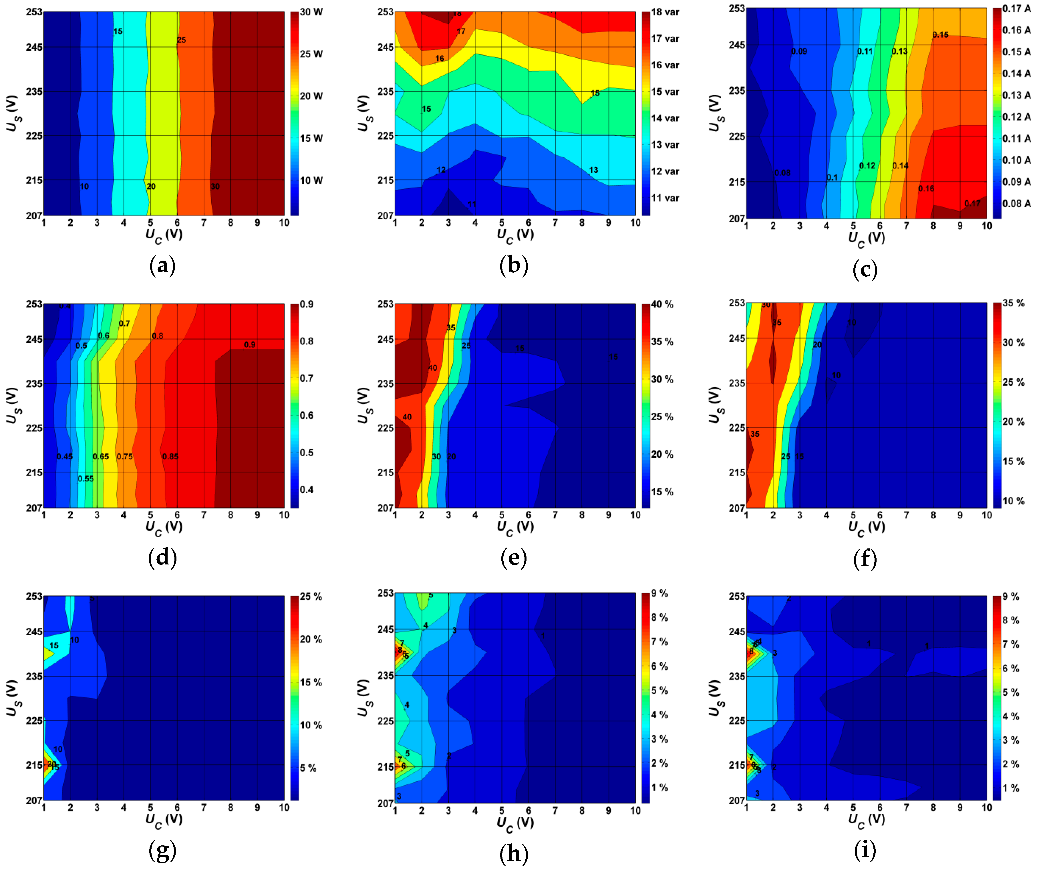
Figure 1a shows changes in the active power of the luminaire as a function of the supply voltage U_S and the control voltage U_C. It shows that the relationship is linear as regards control voltages. In the range U_C = 8–10 V it can be assumed that the luminaire is operating at full power. The value of the active power of the luminaire is practically independent of the supply voltage within the range of variation analysed. The reactive power Q (Figure 1b) increases with a rise in the supply voltage U_S. In contrast to the active power, the reactive power is seen to be strongly dependent on the supply voltage. However, no significant variation in the reactive power is observed depending on the control voltage. Since the current drawn by the luminaire is composed of active and reactive components, it is seen to depend on both the supply and control voltage (Figure 1c).

The luminaire draws its maximum current when it operates at full power and is supplied with a voltage of 207 V. The displacement power factor PF_D as a function of supply voltage and control voltage is shown in Figure 1d. Like other LED luminaires, the tested luminaire has a capacitive power factor for all dimming levels and for the entire range of analysed supply voltages. The power factor is found to be strongly dependent on the control voltage. When the luminaire operates at lower power, the value of this factor decreases, reaching a value of around 0.35 when the supply voltage is 253 V and U_C = 1 V. The next electrical parameter to be analysed is the current distortion factor THD_I (Figure 1e). When THD_I is analysed as a function of the supply voltage U_S and the control voltage U_C, two different zones of variation are observed. For control voltages above 5 V the value of THD_I for current drawn from the network varies over a narrow range. However, as the control voltage falls from 5 V to 1 V, the value of THD_I rises sharply. The maximum value of THD_I is 44.59% (for U_C = 1 V and U_S = 235 V), three times higher than the value obtained when the luminaire operates at full power. Such a large growth in the higher harmonics generated in the supply network may lead to a number of undesirable phenomena, as described widely in the literature [13,18,19,20]. Figure 1f–i show how the higher harmonics of the current of the tested luminaire depend on the voltages U_S and U_C, for the third, ninth, 15th and 21st harmonics respectively. The values of these harmonics are selected because they are used for computation of the power losses in the neutral conductor of the supply cable. The greatest variation can be observed in the case of the third harmonic, which reaches its highest values for control voltages of 1–4 V.

In summary, two ranges of operation of the tested luminaire may be distinguished, based on the value of the control voltage U_C: the first for U_C = 1–5 V, and the second for U_C = 5–10 V. In the first range the current distortion (represented by values of THD_I) is strongly dependent on the dimming level. In the second range there is virtually no such dependence. This leads to the practical conclusion that if it is required that the luminaire should not generate excessive distortions in the supply network in the form of higher current harmonics, then the control voltage should be maintained between 5 V and 10 V. Bearing in mind that in the range U_C = 8–10 V the luminaire operates at full power, the width of the regulating voltage range would then be reduced to 4 V, and the luminaire could be set to operate at between 50 and 100% power. Reducing the range of regulation will reduce variation in the displacement power factor of the luminaire. This is important if the owner of the street lighting system pays for both active and reactive energy consumption, or pays additional charges as a penalty for exceeding the permissible value of the parameter tanϕ.

4. Results of Computations of Power Losses in the Street Lighting System

4.1. Results of Computations of Power Losses in a Three-Phase System

Active power losses were computed for a sample three-phase street lighting system. It was assumed that the number of lamps is 30, giving 10 luminaires per phase. It was also assumed that each luminaire is installed on a separate pole, and that the length of the cable between neighbouring lamps is 30 m. The distance of the first luminaire from the lighting system distribution board was also taken to be 30 m. Cables were assumed to have copper conductors with cross-section 4 × 16 mm² and specific conductance 56 m/Ω·mm². The wire in the pole connecting the fuse box to the luminaire is a copper wire with cross-sectional area 1.5 mm², length 10 m and specific conductance 56 m/Ω·mm². The supply cable is protected with a gG (gL) fuse element with rated current 25 A, with a three-phase fuse base with rated current 160 A. Active power losses for the rated current as stated in the catalogue are 12 W and 2.4 W respectively. The lighting circuit is switched by a relay with rated current 25 A, for which the catalogue power losses for the rated current amount to 7.9 W. The wire connecting the fuse box to the luminaire is protected by a gG (gL) fuse element with rated current 6 A, with a fuse base of rated current 16 A. Power losses for the rated current stated in the manufacturer’s catalogue amount to 1.7 W for the fuse element and 3 W for the base.

Active power losses were computed using the formulae given in Section 2.

Table 1. Power losses ΔP_TOTAL as percentages of the rated power for the three-phase circuit.

Dimming	ΔPTOTAL (%)
	Supply Voltage
	207 V	210 V	215 V	220 V	225 V	230 V	235 V	240 V	245 V	250 V	253 V
1 V	0.40	0.41	0.52	0.46	0.46	0.39	0.45	0.52	0.40	0.40	0.40
2 V	0.32	0.32	0.33	0.34	0.37	0.35	0.41	0.44	0.42	0.43	0.43
3 V	0.22	0.22	0.22	0.22	0.22	0.22	0.27	0.29	0.30	0.32	0.33
4 V	0.24	0.24	0.24	0.23	0.22	0.20	0.22	0.22	0.20	0.22	0.23
5 V	0.26	0.26	0.26	0.25	0.25	0.22	0.23	0.22	0.21	0.21	0.21
6 V	0.29	0.29	0.28	0.27	0.26	0.24	0.25	0.25	0.23	0.22	0.22
7 V	0.32	0.32	0.31	0.30	0.29	0.27	0.27	0.26	0.25	0.24	0.24
8 V	0.35	0.34	0.33	0.32	0.31	0.29	0.30	0.28	0.27	0.26	0.26
9 V	0.34	0.34	0.33	0.32	0.31	0.29	0.29	0.28	0.27	0.26	0.26
10 V	0.35	0.34	0.33	0.32	0.31	0.29	0.29	0.29	0.27	0.26	0.26

gives the losses in the street lighting circuit with 30 luminaires as percentages of the circuit power P_kc, for each dimming level. The circuit power P_kc is the product of the number of lamps n_p and the power of a luminaire P_lum at a given dimming level.

Table 2. Power losses ΔP_a as percentages of the rated power for the three-phase circuit.

Dimming	ΔPa (%)
	Supply Voltage
	207 V	210 V	215 V	220 V	225 V	230 V	235 V	240 V	245 V	250 V	253 V
1 V	0.053	0.053	0.058	0.059	0.060	0.053	0.061	0.062	0.047	0.045	0.043
2 V	0.070	0.069	0.068	0.066	0.081	0.073	0.078	0.084	0.062	0.060	0.060
3 V	0.099	0.099	0.098	0.099	0.097	0.095	0.112	0.119	0.087	0.084	0.083
4 V	0.137	0.141	0.134	0.133	0.128	0.120	0.126	0.130	0.106	0.103	0.102
5 V	0.172	0.171	0.171	0.169	0.161	0.149	0.155	0.150	0.130	0.126	0.121
6 V	0.209	0.209	0.199	0.193	0.190	0.176	0.183	0.176	0.159	0.149	0.146
7 V	0.246	0.242	0.234	0.226	0.222	0.204	0.206	0.201	0.182	0.173	0.170
8 V	0.279	0.272	0.264	0.255	0.245	0.233	0.235	0.226	0.206	0.197	0.193
9 V	0.277	0.272	0.267	0.256	0.248	0.233	0.232	0.226	0.206	0.197	0.192
10 V	0.283	0.276	0.265	0.257	0.249	0.233	0.235	0.229	0.206	0.197	0.193

and

Table 3. Power losses ΔP_r as percentages of the rated power for the three-phase circuit.

Dimming	ΔPr (%)
	Supply Voltage
	207 V	210 V	215 V	220 V	225 V	230 V	235 V	240 V	245 V	250 V	253 V
1 V	0.349	0.362	0.462	0.399	0.405	0.333	0.386	0.461	0.355	0.353	0.355
2 V	0.252	0.254	0.258	0.274	0.291	0.274	0.328	0.357	0.356	0.372	0.368
3 V	0.122	0.122	0.123	0.120	0.126	0.128	0.155	0.172	0.217	0.239	0.248
4 V	0.105	0.104	0.101	0.093	0.094	0.085	0.091	0.093	0.096	0.114	0.128
5 V	0.092	0.089	0.089	0.080	0.085	0.075	0.076	0.073	0.080	0.082	0.085
6 V	0.082	0.081	0.076	0.077	0.073	0.069	0.070	0.069	0.072	0.074	0.075
7 V	0.073	0.073	0.073	0.070	0.070	0.064	0.064	0.061	0.067	0.069	0.070
8 V	0.069	0.067	0.065	0.063	0.064	0.059	0.061	0.057	0.063	0.065	0.065
9 V	0.068	0.066	0.066	0.064	0.064	0.060	0.059	0.058	0.063	0.065	0.066
10 V	0.069	0.068	0.066	0.065	0.064	0.060	0.059	0.058	0.063	0.065	0.065

give the active power losses caused by the flow of active and reactive power respectively.

The percentage total losses relative to the circuit power are found to take their highest values (from 0.4 to 0.52%) at the control voltage U_C = 1 V (Figure 2a). When the luminaire operates at full power, these losses lie between 0.26 and 0.35%. The flow of active current through elements of the supply network leads to active power losses caused by the flow of active power ΔP_a. The flow of reactive current leads to active power losses caused by the flow of reactive power ΔP_r. This is described by the following equations:

$$\Delta P=\left(S^2/U_r\right)/R=\left(\left(P^2/U_r\right)/R\right)+\left(\left(Q^2/U_r\right)/R\right)=\Delta P_a+\Delta P_r,$$

(20)

$$\Delta P_r=\Delta P_a{\mathrm{tg}}^2\varphi ,$$

(21)

Table 2 and Table 3 contain values of active power losses caused by the flow of active and reactive power respectively. As the power factor decreases—that is, as the power of the luminaire decreases—there is an increase in the percentage value of active power losses caused by the flow of reactive power. For control voltages in the range 1–3 V, these losses are dominant. For control voltages of 4 V upwards, active power losses caused by the flow of active power begin to take larger values. It can be seen from Figure 2b and Table 2 that the losses ΔP_a depend both on the dimming level and on the supply voltage. For the losses ΔP_r (Figure 2c) the dependence on the supply voltage is smaller than in the case of ΔP_a. Losses in the neutral conductor caused by the flow of higher current harmonics were treated as active power losses.

For all elements of the supply network for which the active power losses were analysed, there is a clear region in which the losses are not dependent on the control voltage U_c or the supply voltage U_s (Figure 3). This is the region where U_c ranges from 3 V to 10 V. When U_c is below 3 V, the contributions of individual components to the total active power losses are strongly dependent on both the supply voltage U_s and on the control voltage. The dominant contributions to the total losses are those of the supply cable (up to 90%) and the neutral conductor (up to 30%).

4.2. Results of Computations of Power Losses in a Single-Phase System

Computations of active power losses were also made for a single-phase street lighting system consisting of 30 lamps. It was assumed that the length of the cable, with 2 × 25 mm² copper conductors, between the luminaires is equal to 30 m, and that the distance of the first luminaire from the distribution board is also 30 m. As in the case of the three-phase system, it was assumed that the wire in the pole connecting the fuse box to the luminaire is a copper wire with cross-sectional area 1.5 mm² and length 10 m. The supply cable is protected by a gG (gL) fuse element with rated current 25 A, with a single-phase fuse base with rated current 160 A. The active power losses for the rated current given in the manufacturer’s catalogue are 12 W and 2.4 W respectively. It was also assumed that the lighting circuit is switched by a relay with rated current 25 A, for which the catalogue power losses for the rated current amount to 7.9 W. The wire in the pole is protected by a gG (gL) fuse element with rated current 6 A, with a fuse base with rated current 16 A. Power losses for the rated current as stated in the catalogue are 1.7 W for the fuse element and 3 W for the base.

Computations of active power losses were again performed using the formulae given in Section 2.

Table 4. Power losses ΔP_TOTAL as percentages of the rated power for the single-phase circuit.

Dimming	ΔPTOTAL (%)
	Supply Voltage
	207 V	210 V	215 V	220 V	225 V	230 V	235 V	240 V	245 V	250 V	253 V
1 V	1.86	1.88	2.04	2.08	2.12	1.86	2.15	2.18	2.00	2.04	2.07
2 V	1.60	1.61	1.59	1.63	1.76	1.59	1.86	1.99	1.84	1.87	1.87
3 V	1.26	1.26	1.25	1.24	1.25	1.18	1.36	1.44	1.46	1.52	1.54
4 V	1.35	1.37	1.32	1.28	1.26	1.16	1.24	1.26	1.13	1.17	1.21
5 V	1.47	1.45	1.45	1.39	1.38	1.26	1.31	1.27	1.20	1.19	1.17
6 V	1.64	1.62	1.55	1.51	1.47	1.37	1.42	1.38	1.30	1.27	1.26
7 V	1.80	1.78	1.72	1.67	1.64	1.50	1.51	1.48	1.40	1.36	1.35
8 V	1.97	1.92	1.87	1.80	1.74	1.64	1.66	1.59	1.52	1.48	1.45
9 V	1.96	1.92	1.88	1.81	1.75	1.64	1.64	1.60	1.52	1.47	1.45
10 V	2.00	1.95	1.87	1.82	1.76	1.64	1.66	1.61	1.51	1.47	1.45

gives the power losses in the street lighting circuit with 30 luminaires, as percentages of the circuit power P_kc for each dimming level.

Table 5. Power losses ΔP_a as percentages of the rated power for the single-phase circuit.

Dimming	ΔPa (%)
	Supply Voltage
	207 V	210 V	215 V	220 V	225 V	230 V	235 V	240 V	245 V	250 V	253 V
1 V	0.308	0.310	0.341	0.346	0.348	0.310	0.356	0.360	0.275	0.261	0.254
2 V	0.407	0.404	0.400	0.387	0.474	0.425	0.454	0.493	0.365	0.351	0.352
3 V	0.581	0.579	0.571	0.582	0.565	0.556	0.658	0.696	0.507	0.489	0.483
4 V	0.804	0.826	0.782	0.780	0.748	0.700	0.738	0.759	0.620	0.603	0.599
5 V	1.006	1.002	0.998	0.986	0.943	0.870	0.907	0.879	0.758	0.739	0.710
6 V	1.224	1.221	1.166	1.130	1.112	1.029	1.069	1.031	0.928	0.873	0.853
7 V	1.438	1.419	1.369	1.325	1.300	1.191	1.206	1.176	1.064	1.009	0.993
8 V	1.634	1.591	1.546	1.490	1.436	1.363	1.372	1.320	1.205	1.155	1.127
9 V	1.620	1.590	1.560	1.499	1.453	1.362	1.358	1.324	1.204	1.153	1.126
10 V	1.656	1.617	1.549	1.505	1.454	1.362	1.373	1.338	1.203	1.152	1.126

and

Table 6. Power losses ΔP_r as percentages of the rated power for the single-phase circuit.

Dimming	ΔPr (%)
	Supply Voltage
	207 V	210 V	215 V	220 V	225 V	230 V	235 V	240 V	245 V	250 V	253 V
1 V	1.556	1.567	1.703	1.734	1.776	1.547	1.798	1.817	1.724	1.783	1.817
2 V	1.190	1.204	1.187	1.243	1.288	1.169	1.401	1.494	1.477	1.524	1.516
3 V	0.678	0.682	0.677	0.662	0.683	0.627	0.707	0.748	0.950	1.028	1.057
4 V	0.547	0.543	0.539	0.497	0.511	0.461	0.503	0.500	0.512	0.572	0.615
5 V	0.466	0.451	0.453	0.404	0.436	0.387	0.403	0.391	0.440	0.448	0.464
6 V	0.413	0.403	0.382	0.382	0.361	0.342	0.354	0.353	0.376	0.393	0.403
7 V	0.365	0.361	0.355	0.343	0.336	0.310	0.307	0.301	0.340	0.353	0.357
8 V	0.337	0.328	0.320	0.309	0.303	0.282	0.285	0.271	0.313	0.322	0.326
9 V	0.335	0.327	0.323	0.308	0.301	0.282	0.282	0.273	0.313	0.321	0.327
10 V	0.342	0.334	0.319	0.312	0.301	0.282	0.283	0.277	0.311	0.322	0.326

contain the computed active power losses caused by the flow of active power (ΔP_a) and reactive power (ΔP_r) as percentages of the rated power of the single-phase circuit. For supply voltages below 215 V, the loss percentage is smallest for control voltages from 3 V to 5 V, ranging between 1.3 and 1.5%. In the case of control voltages below 3 V or above 5 V the percentage is greater, reaching 2% (Table 4). For supply voltages above 215 V the loss percentage takes minimum values for control voltages in the range 3–5 V. For the lowest analysed control voltage (1 V) the percentage loss is largest, exceeding 2%.

Analysing the components of the losses (Table 5 and Table 6) it is seen that the primary factor determining the component percentage values is the control voltage U_c. As U_c rises from 1 V to 10 V these values may change several fold: for example, ΔP_a for U_s = 230 V varies from 0.31% to 1.36%. Values of ΔP_a are highest for operation at full power, while the reverse holds for P_r. For ΔP_r a slight effect is exerted by changes in the value of the supply voltage U_s, but this is negligible compared with the effect of the control voltage U_c. For ΔP_a, when the control voltage is above 5 V, the percentage loss becomes dependent on the supply voltage U_s, being greatest when U_s takes its lowest value. These relationships are shown on contour diagrams in Figure 4. These make it easy to observe the percentage value of a given component depending on the dimming level and the supply voltage.

Power losses in elements of the lighting system as percentages of the total losses ΔP_TOTAL for three-phase network shown in Figure 5a. For the single-phase system, the largest component of the losses is the loss occurring in the supply cable (97%). The remaining components are approximately equal at around 1% (Figure 5b).

The figures show the percentage share of power losses in the devices calculated for 230 V voltage and a lighting installation composed of 30 luminaires for 100% dimming.

5. Mathematical Model of a Luminaire for Computation of Active Power Losses

To compute power losses in a three-phase network, it is sufficient to have knowledge of parameters of the regulated luminaire such as the active power, power factor and reactive power. If the computations of active power losses for a three-phase network are to take account of losses in the neutral conductor, then it is also necessary to have knowledge of the harmonic currents in the zero sequence with orders being multiples of three.

As has been shown in the foregoing chapters, the electrical parameters of a luminaire and the active power losses depend on two variables: the supply voltage U_S and the dimming control voltage U_C. Using the developed model it is possible to determine the parameters of the luminaire which will serve as input data for the computation of active power losses in the lighting system, namely the active power P, the displacement power factor PF_D, the RMS supply current I, and the RMS values of the current harmonics I_hn, where n is the order of the harmonic. A luminaire, as a nonlinear electrical load, is a source of higher harmonics of the supply current [13,19,20].

The developed model enables computation of the electrical parameters of a luminaire for control voltages in the range 1–10 V and supply voltages in the range 207–253 V. The voltages in a real distribution network usually lie between these limits. Using the model, the active power losses may be determined for any supply voltage from this range and for any dimming level. In this way one may compute both the power losses and the power of the lighting system as a whole. These data will enable precise calculation of the energy efficiency of the street lighting system. Using the method of linear regression, based on the measurement data, approximating polynomials were determined for electrical parameters such as the active power and the displacement power factor PF_D (cosϕ) [21,22,23,24]. Approximating polynomials for the active power of the luminaire, the power factor and the RMS supply current are given in

Table 7. Form of the approximating polynomials for analysed parameters.

Parameter	Form of Polynomial
Active power P	P(UC,US) = 22.91 + 12.41UC − 0.03646US − 0.9593UC2 − 0.0223UCUS − 1.608UC3 − 0.001888UC2US − 0.2163UC4 − 0.002771UC3US
Displacement power factor PFD	PF(UC,US) = −0.8639 − 0.08082UC + 0.003243US + 0.1204UC2 − 0.01196UCUS + 0.01532US2 − 0.09274UC3 + 0.01069UC2US − 0.01501UCUS2 + 0.006405US3 − 0.01472UC4 + 0.005266UC3US − 0.001153UC2US2 − 0.001942UCUS3 + 0.02446UC5 − 0.00424UC4US + 0.005417UC3US2 − 0.000624UC2US3
RMS current I	I(UC,US) = −689.7 + 3.472UC + 14.87US − 0.01839UC2 − 0.05933UCUS − 0.128US2 + 0.0001402UC3 + 0.0002673UC2US + 0.0003809UCUS2 + 0.0005504US3 − 7.59 × 10−5UC4 − 4.929 × 10−7UC3US − 9.726 × 10−7UC2US2 − 1.093 × 10−6UCUS3 − 1.182 × 10−6US4 + 1.364 × 10−5UC5 − 1.458e × 10−6UC4US + 7.956 × 10−8UC3US2 − 7.331 × 10−10UC2US3 + 1.199 × 10−9UCUS4 + 1.013 × 10−9US5

below. For the mathematical description of these phenomena one may use models of a nonlinear load based, for example, on its design [16,25,26]. The method given here for determining power losses may be used not only for luminaires, but also for other load devices with nonlinear current-voltage characteristics [18,27,28,29,30].

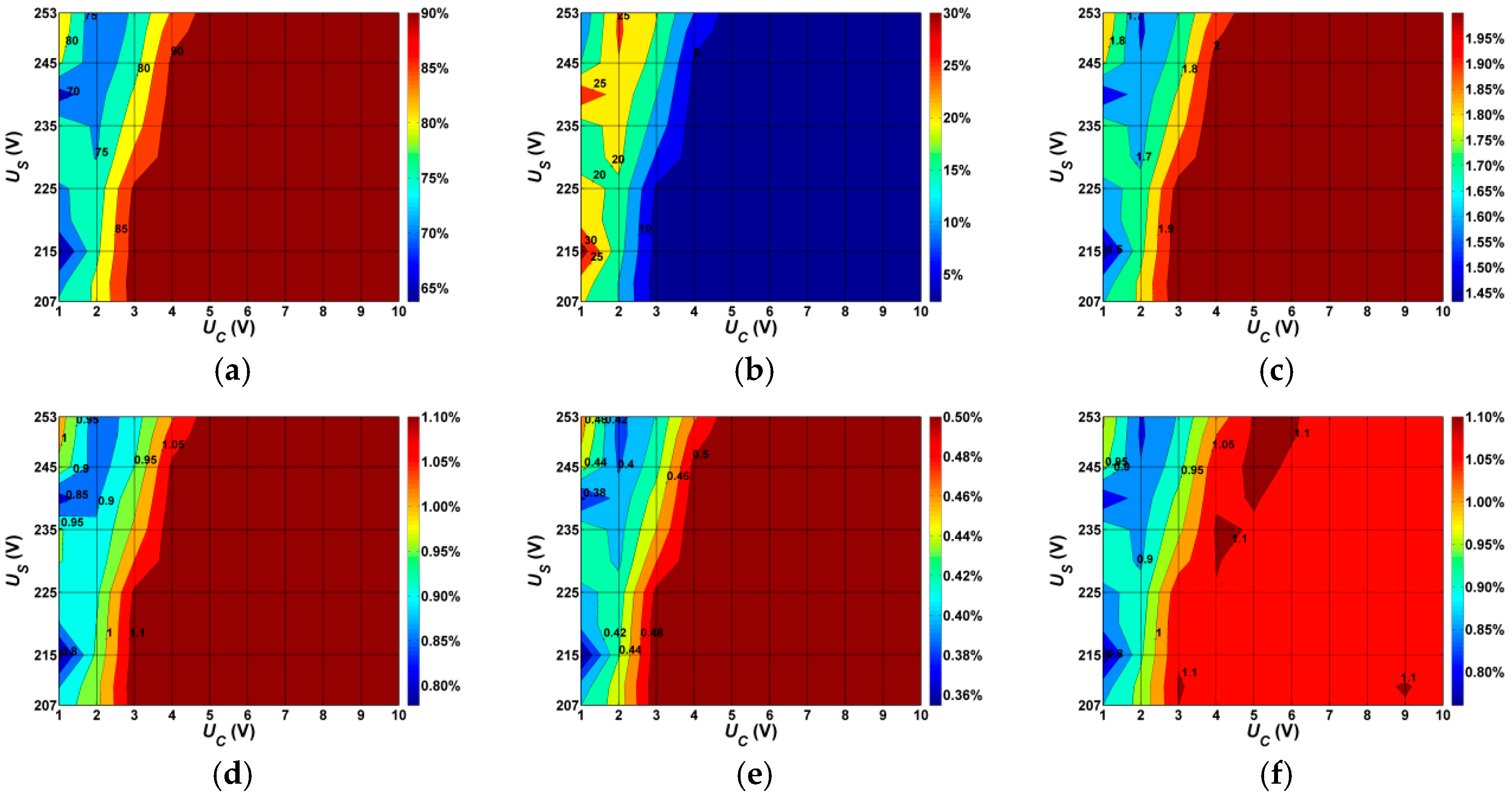
The mean square error R² for the polynomial approximating the value of the active power as a function of the voltages U_C and U_S is 0.9979. For the polynomial approximating the displacement power factor PF_D(U_C,U_S) we have R² = 0.9953, and for the polynomial approximating the value of the RMS current we have R² = 0.9967.

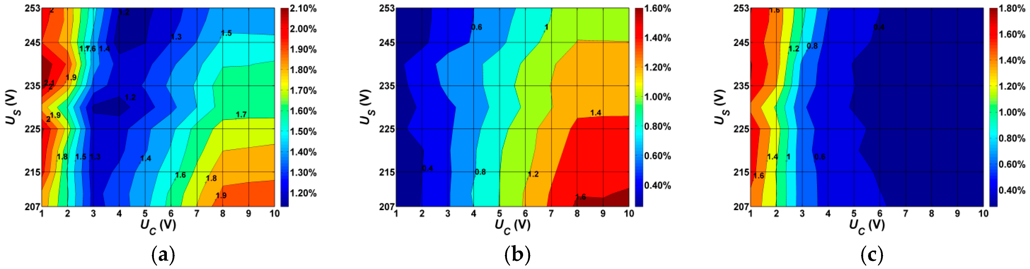
In the computations of power losses, account is taken of such harmonics as I_h3, I_h9, I_h15, I_h21, I_h27, I_h33 and I_h39. The even harmonics are neglected, since they take only small values. Linear regression was used to determine approximating polynomials for these values, but the results were not satisfactory: the R² error exceeded the set limit of 10%. For this reason, to model the harmonics, the method of cubic spline interpolation was used. The matrix notation for cubic spline interpolation is:

$$\left[x\left(u\right)y\left(u\right)z\left(u\right)\right]=\left[u^3{u}^{2}u\right]\left[\begin{array}{ccc}{a}_x& a_y& a_z\\ b_x& b_y& b_z\\ c_x& c_y& c_z\\ d_x& d_y& d_z\end{array}\right],$$

(22)

or:

$$P=UA,$$

(23)

where:

$$P=\left[x\left(u\right)y\left(u\right)z\left(u\right)\right],$$

(24)

$$U=\left[u^3{u}^{2}u\right],$$

(25)

$$A=\left[\begin{array}{ccc}{a}_x& a_y& a_z\\ b_x& b_y& b_z\\ c_x& c_y& c_z\\ d_x& d_y& d_z\end{array}\right],$$

(26)

This method enabled the prediction of higher current harmonics with an accuracy that was adequate from a practical point of view. For regressions of this type, the mean square errors R² are equal to 1.

Using the developed model, electrical parameters may be determined for any supply voltage U_S in the range 230 V ±10% and for dimming levels ranging from 10% to full power. Computations were performed for sample input data; the results are given in

Table 8. Parameters of a luminaire computed using the model.

US	UC	P	I	cosϕ	Ih3	Ih9	Ih15	Ih21	Ih27	Ih33	Ih39
(V)	(V)	(W)	(mA)	(-)	(mA)	(mA)	(mA)	(mA)	(mA)	(mA)	(mA)
209	5.5	22.96	128.27	0.856	16.01	1.80	1.23	1.36	0.98	0.90	0.90
218	4.5	18.58	105.63	0.815	12.96	1.51	1.72	1.00	1.18	0.98	0.88
227	6.2	25.85	132.33	0.878	16.22	2.23	1.09	0.92	0.98	0.68	0.74
238	7.2	29.50	143.74	0.886	17.03	2.20	1.32	1.44	1.11	0.97	1.02
247	5.2	19.83	104.29	0.791	9.91	2.32	1.21	0.63	0.64	0.44	0.42

. In practical computations, account must be taken of the illumination schedule defined for the luminaires and the consequent dimming levels, which must comply with the illumination requirements for the road in question, in accordance with the standard [9]. Values of the RMS supply voltage result from the conditions of the power supply to the lighting system distribution board.

Knowing the values of the electrical parameters for the assumed values of U_S and U_C, it is possible to determine the separate components of the active power losses. To do this, the concrete numerical values of the electrical parameters given in Table 8 were substituted into Equations (3)–(19). The results of the computations appear in

Table 9. Computed power losses.

US	UC	ΔPTOTAL	ΔPa	ΔPr	ΔPCABLE	ΔPNEUTRAL	ΔPWIRE	ΔPPPB	ΔPPPOLE	ΔPRELAY
(V)	(V)	(%)	(%)	(%)	(%)	(%)	(%)	(%)	(%)	(%)
209	5.5	0.28	0.20	0.08	90.88	4.38	2.04	1.11	0.51	1.08
218	4.5	0.23	0.15	0.08	90.94	4.32	2.04	1.11	0.51	1.08
227	6.2	0.26	0.19	0.07	91.03	4.23	2.05	1.11	0.51	1.09
238	7.2	0.27	0.20	0.07	91.26	3.98	2.05	1.11	0.51	1.09
247	5.2	0.21	0.13	0.08	92.48	2.70	2.08	1.13	0.51	1.10

.

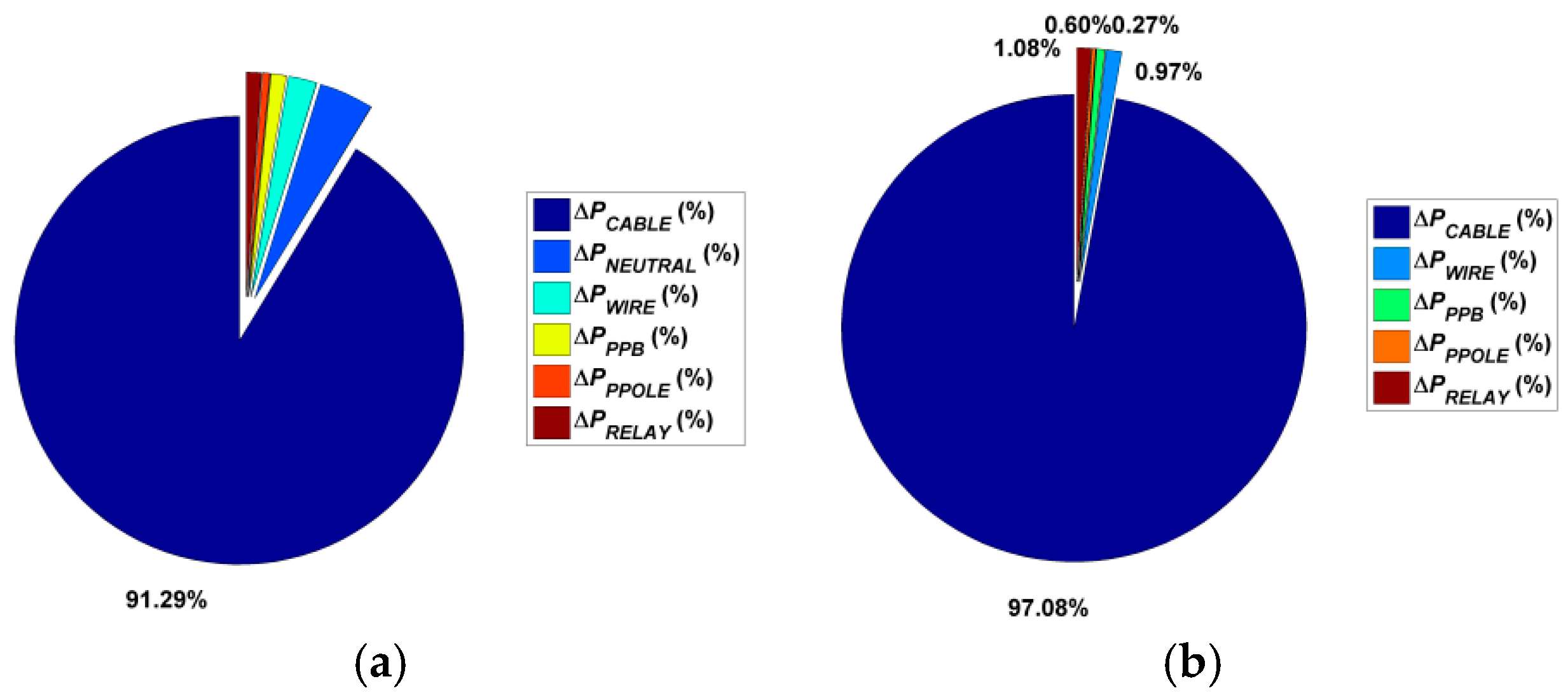
The values of ΔP_TOTAL, ΔP_a and ΔP_r are expressed as percentages of the rated power for the analysed lighting system (30 luminaires). For the remaining parameters, the values represent the percentage contributions of the individual components to the total power losses.

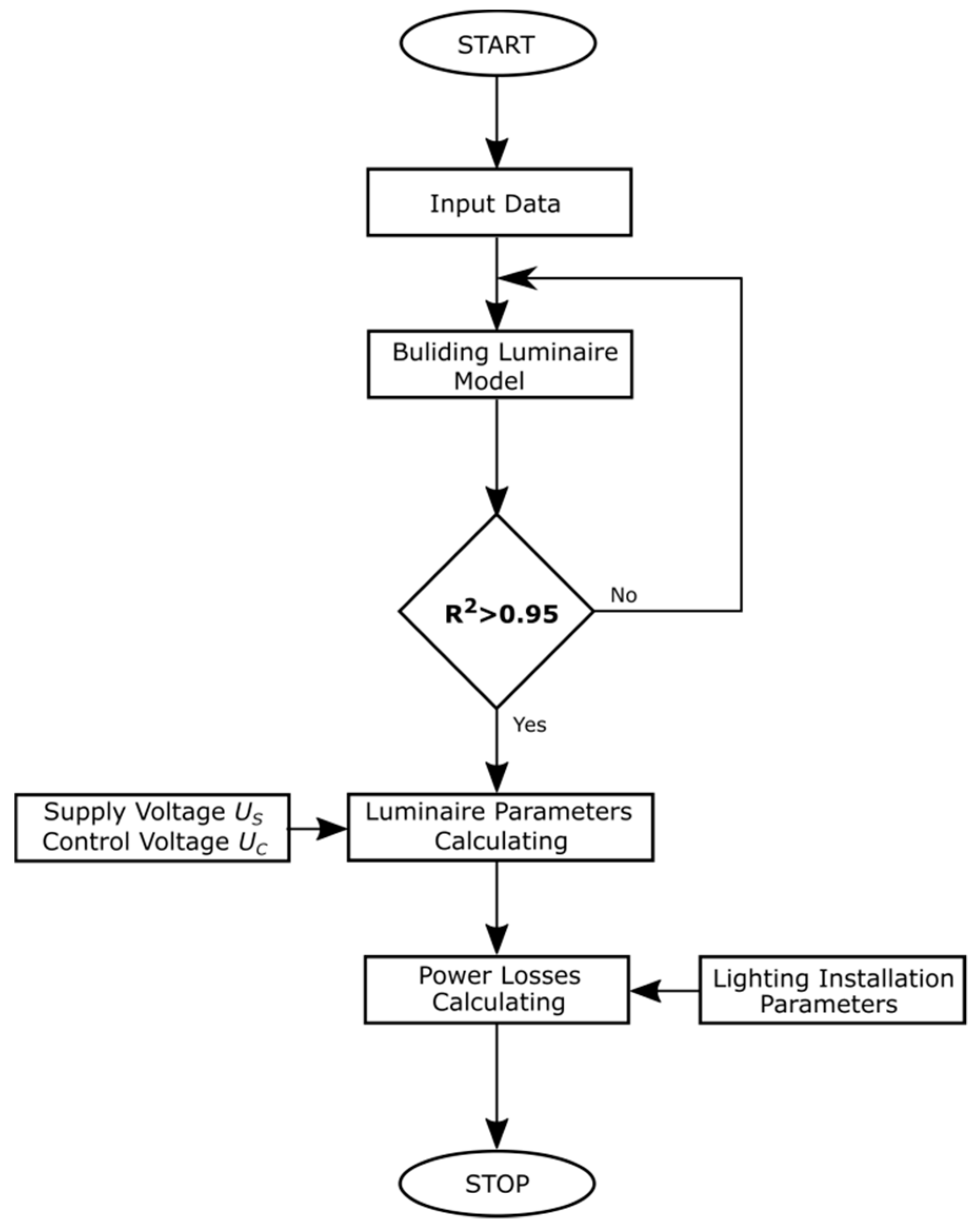
Figure 6 shows the proposed method of determining total losses using the developed model, in the form of an algorithm. The input data are the measured characteristics of changes in the analysed basic electrical parameters depending on the value of the RMS supply voltage and the dimming level. The range of variation of the supply voltage results from the requirements of the EN 50160 standard [16], and the considered variation in the dimming level should cover the complete range available for the luminaire. For obvious reasons, increasing the number of analysed points improves the accuracy of the computed characteristics, but at the cost of increasing the quantity of work. To obtain a desired accuracy of 5%, the number of measurement points given in Table 4 can be considered sufficient.

At the next stage, a mathematical model of the luminaire is constructed, and the mean square error value is checked. If the error exceeds the set limit, the construction process is repeated with an adjustment to the degree of the approximating polynomials, or else a different regression method is adopted. At the start of model construction the degrees of the polynomials are taken as small as possible; higher-degree polynomials are used if the accuracy needs to be improved. When the mean square error is found to be at an acceptable level, work on the construction of the model is complete. For any values of the input data (U_S and U_c) the model can be used to determine the electrical parameters; sample values of these are given in Table 8. Based on the parameters of the lighting system, particular components of the active power losses may be determined (sample values appear in Table 9) based on the analytical equations given in Section 2. The parameters of the lighting system include values such as the number of lamps, the power of each lamp, the cross-sectional area, length and type of the supply cables, and so on.

6. Conclusions

Any lighting system ought to offer high energy efficiency. Lighting is an area in which efficiency can be significantly improved by means of a relatively small amount of financial expenditure. Section 5 of the standard [6] defines indicators for evaluation of the energy efficiency of street lighting, taking account of the consumption of energy while adequate street lighting parameters are maintained. One of the indicators for evaluation of the energy efficiency of a lighting system is the power density D_P. This value is directly proportional to the active power of the system, and inversely proportional to the value of the mean illuminance and illuminated area. One of the components of the active power, alongside the utilised power of the luminaires, is the active power losses occurring in the various components of the system. With regard to the possibility of using luminaires with regulated power, operating according to a defined schedule, it is necessary to choose the technical solution that will provide the best energy efficiency. Analysis of the energy efficiency of street lighting in accordance with the PN-EN 13201 standard [9] requires knowledge of the mean illuminance on the road, the size of the illuminated area, and the power of the lighting system under consideration. Computations are usually performed based on the rated powers of the luminaires, neglecting power losses in the devices of which the system is composed. An increase in power losses will lead to an increase in the active power consumed, and in the cost of the electricity used. Failure to take account of this factor in energy audits may lead to discrepancies between the computed theoretical values and the actual values of active power consumed. An increase in power losses will cause a reduction in the DP factor. that is with the deterioration of energy efficiency of the lighting installation.

This article has described a method of determining the power losses occurring in a lighting system, depending on the power supply conditions and the dimming level. The components of active power losses and analytical methods for their determination are introduced in Section 2. The method used to determine the losses is dependent on the configuration of the supply network, that is, whether it is single-phase or three-phase. Total active power losses are presented here as the sum of individual components, such as the losses in the working conductors of the supply cable, in the neutral conductor for three-phase systems, and in other devices of the power supply system. Since the proposed method of determining losses is based on a mathematical model, Section 3 contains a presentation of results of measurements to determine how the electrical parameters of a luminaire, such as the active power P, the reactive power Q and the factor THD_I, depend on the RMS supply voltage and the dimming level. Construction of the mathematical model for a luminaire involves the use of an approximating polynomial [21,22,29,31] or cubic spline interpolation, depending on the output parameter being analysed. Section 4 includes sample results of computations of active power losses, including values for the losses resulting from the flow of active and reactive power. These computations were performed for assumed parameters of the lighting system. The algorithm for construction of the model is described in detail in Section 5. Results are given for computations of active power losses for arbitrary values of the supply voltage and the dimming level of the luminaire. The algorithm is shown in diagram form in Figure 6. Given the mathematical model for a luminaire, one may determine the level of losses for any chosen value of RMS supply voltage U_S and dimming level (control voltage) U_C, and thereby, for example, select a dimming regulation schedule in such a way as to minimise those losses. This means that, during the design of the system, it becomes possible to select a solution offering the highest energy efficiency, and consequently the lowest operating costs.

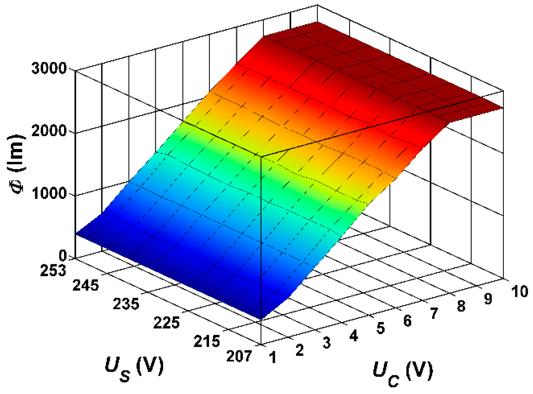
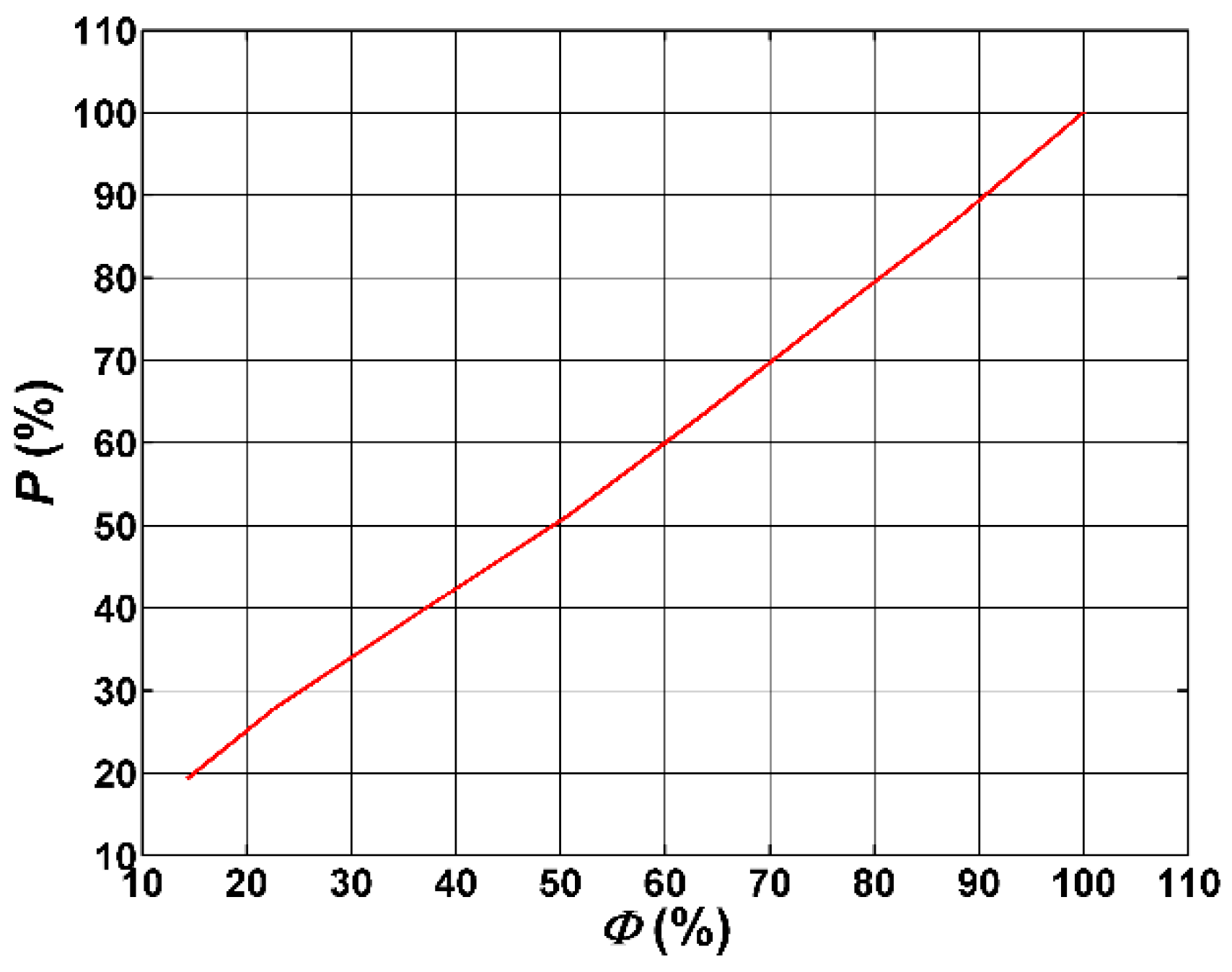
The characteristics of the luminous flux of the tested luminaire as a function of the control voltage U_C and the supply voltage U_S are shown in Figure 5. In the range of control voltages from 1 V to 8 V, the luminous flux increases linearly to the full value (Figure 7). For U_C voltages ≥ 8 V, the luminous flux does not change. The relationship between the percentage of active power and the luminous flux of the luminaire considered is shown in the Figure 8. This dependence is linear.

References

1. Kostic, M.; Djokic, L. Recommendations for energy efficient and visually acceptable street lighting. Energy 2009, 34, 1565–1572. [Google Scholar] [CrossRef]
2. Ożadowicz, A.; Grela, J. Energy saving in the street lighting control system—A new approach based on the EN-15232 standard. Energy Effic. 2017, 10, 563–576. [Google Scholar] [CrossRef]
3. Gutierrez-Escolar, A.; Castillo-Martinez, A.; Gomez-Pulido, J.M.; Gutierrez-Martinez, J.M.; Dominguez González-Seco, E.P.; Stapic, Z. A review of energy efficiency label of street lighting systems. Energy Effic. 2017, 10, 265–282. [Google Scholar] [CrossRef]
4. Hermoso Orzáez, M.J.; de Andrés Díaz, J.R. Comparative study of energy-efficiency and conservation systems for ceramic metal-halide discharge lamp. Energy 2013, 52, 258–264. [Google Scholar] [CrossRef]
5. Lobão, J.A.; Devezas, T.; Catalão, J.P.S. Energy efficiency of lighting installations: Software application and experimental validation. Energy Rep. 2015, 1, 110–115. [Google Scholar] [CrossRef]
6. Pinto, M.F.; Soares, G.M.; Mendonça, T.R.F.; Almeida, P.S.; Braga, H.A.C. Smart Modules for Lighting System Applications and Power Quality Measurements. In Proceedings of the 11st IEEE/IAS International Conference on Industry Applications (INDUSCON), Juiz de Fora, Brazil, 7–10 December 2014. [Google Scholar]
7. Todorović, B.M.; Samardžija, D. Road lighting energy-saving system based on wireless sensor network. Energy Effic. 2016, 10, 1–9. [Google Scholar] [CrossRef]
8. Yan, W.; Hui, S.Y.R.; Chung, H.S.-H. Energy Saving of Large-Scale High-Intensity-Discharge Lamp Lighting Networks Using a Central Reactive Power Control System. IEEE Trans. Ind. Electron. 2009, 56, 3069–3078. [Google Scholar] [CrossRef]
9. Oświetlenie Dróg; PN-EN 13201:2016; Polski Komitet Normalizacyjny: Warszawa, Polska, 2016.
10. Radulovic, D.; Skok, S.; Kirincic, V. Energy efficiency public lighting management in the cities. Energy 2011, 36, 1908–1915. [Google Scholar] [CrossRef]
11. Lobão, J.A.; Devezas, T.; Catalão, J.P.S. Influence of cable losses on the economic analysis of efficient and sustainable electrical equipment. Energy 2014, 65, 145–151. [Google Scholar] [CrossRef]
12. Vysotsky, V.S.; Nosov, A.A.; Fetisov, S.S.; Shutov, K.A. AC Loss and Other Researches with 5 m HTS Model Cables. IEEE Trans. Appl. Supercond. 2011, 21, 1001–1004. [Google Scholar] [CrossRef]
13. Jettanasen, C.; Pothisarn, C. Analytical Study of Harmonics Issued from LED Lamp Driver. In Proceedings of the International MultiConference of Engineers and Computer Scientists, Hong Kong, China, 12–14 March 2014. [Google Scholar]
14. Mekhamer, S.F.; El-Hawary, M.E.; Soliman, S.A.; Moustafa, M.A.; Mansour, M.M. New Heuristic Strategies for Reactive Power Compensation of Radial Distribution Feeders. IEEE Trans. Power Deliv. 2002, 17, 1128–1135. [Google Scholar] [CrossRef]
15. EN. 50160: Voltage Characteristics of Electricity Supplied by Public Distribution Systems; British Standards Institution: London, UK, 2007. [Google Scholar]
16. Acarkan, B.; Zorlu, S.; Kilic, O. Nonlinear Resistance Modeling Using MATLAB and Simulink in Estimation of City Street Lighting Harmonic Activity. In Proceedings of the International Conference on Computer as a Tool, Belgrade, Serbia, 22–24 November 2005; p. 1251. [Google Scholar]
17. Gabryjelski, Z.; Kowaski, Z. Sieci I Urządzenie Oświetleniowe: Zagadnienia Wybrane, 1st ed.; Wydawnictwo Politechniki Łódzkiej: Łódź, Poland, 1997; pp. 118–127. ISBN 83-86453-95-8. [Google Scholar]
18. Mansoor, A.; Grady, W.M.; Chowdhury, A.H.; Samotyj, M.J. An Investigation of Harmonics Attenuation and Diversity Among Distributed Single-Phase Power Electronic Loads. IEEE Trans. Power Deliv. 1994, 10, 467–473. [Google Scholar] [CrossRef]
19. Pabjańczyk, W.; Sikora, R.; Markiewicz, P. Study of electrical parameters of road luminaires. Logistyka 2014, 6, 8270–8276. [Google Scholar]
20. Pabjańczyk, W.; Sikora, R.; Markiewicz, P. Modelling and simulations of street lighting installations. Logistyka 2014, 6, 8260–8269. [Google Scholar]
21. Aikio, J.P.; Rahkonen, T. Polynomial fitting of nonlinear sources with correlating inputs. Int. J. Comput. Math. Electr. Electron. Eng. 2012, 33, 1097–1106. [Google Scholar] [CrossRef]
22. Rust, B.W. Fitting nature’s basic functions part I: Polynomials and linear least squares. IEEE Comput. Sci. Eng. 2001, 3, 84–89. [Google Scholar] [CrossRef]
23. Rust, B.W. Fitting nature’s basic functions part II: Estimating uncertainties and testing hypotheses. IEEE Comput. Sci. Eng. 2001, 3, 60–64. [Google Scholar] [CrossRef]
24. Taubin, G. An improved algorithm for algebraic curve and surface fitting. In Proceedings of the Fourth International Conference on Computer Vision, Berlin, Germany, 11–14 May 1993; pp. 658–665. [Google Scholar]
25. Herraiz, S.; Sainz, L.; Pedra, J. Behavior of single-phase full-wave rectifier. Eur. Trans. Electr. Power 2003, 13, 185–192. [Google Scholar] [CrossRef]
26. Herraiz, S.; Sainz, L.; Pedra, J. Unified and simple model for uncontrolled rectifiers. Electr. Power Syst. Res. 2005, 74, 331–340. [Google Scholar] [CrossRef]
27. Grasselli, U.; Lamedica, R.; Prudenzi, A. Characterization of fluctuating harmonics from single-phase power electronics-based equipment. Int. J. Comput. Math. Electr. Electron. Eng. 2015, 23, 133–147. [Google Scholar] [CrossRef]
28. Mesas, J.J.; Sainz, L.; Sala, P. Statistical study of personal computer cluster harmonic currents from experimental measurements. Electr. Power Compon. Syst. 2015, 43, 56–68. [Google Scholar] [CrossRef] [Green Version]
29. Mujovic, S.; Djukanovic, S.; Radulovic, V. Multi-parameter mathematical model for determination of PC cluster total harmonic distortion of input current. Int. J. Comput. Math. Electr. Electron. Eng. 2016, 35, 305–325. [Google Scholar] [CrossRef]
30. Nassif, A.B.; Yong, J.; Xu, W.; Chung, C.Y. Indices for comparative assessment of the harmonic effect of different home appliances. Int. Trans. Electr. Energy Syst. 2013, 23, 638–654. [Google Scholar] [CrossRef]
31. The MathWorks, Inc. Curve Fitting Toolbox™ User’s Guide; The MathWorks Inc.: Natick, MA, USA, 2002. [Google Scholar]
Figure 1. Measured electrical parameters of the luminaire: (a) active power P; (b) reactive power Q; (c) IRMS; (d) displacement power factor PFD; (e) THDI; (f) Ih3; (g) Ih9; (h) Ih15; (i) Ih21.
Energies 11 01386 g001
Figure 2. Active power losses in a street lighting circuit with 30 luminaires as percentages of the circuit power Pkc: (a) total power losses ΔPTOTAL; (b) active power losses caused by flow of active power ΔPa, (c) active power losses caused by flow of reactive power ΔPr.
Energies 11 01386 g002
Figure 3. Power losses in elements of the lighting system as percentages of total power losses ΔPTOTAL: (a) losses in the supply cable; (b) losses in the neutral conductor of the supply cable; (c) losses in the wire in the pole between the fuse box and the luminaire; (d) losses in the safety device in the distribution board; (e) losses in the safety device of the wire in the pole; (f) losses in the relay.
Energies 11 01386 g003
Figure 4. Active power losses in a street lighting circuit with 30 luminaires as percentages of the circuit power Pkc: (a) total power losses ΔPTOTAL; (b) active power losses caused by the flow of active power ΔPa; (c) active power losses caused by the flow of reactive power ΔPr.
Energies 11 01386 g004
Figure 5. Power losses in elements of the lighting system as percentages of the total losses ΔPTOTAL for (a) three-phase system, (b) single-phase system.
Energies 11 01386 g005
Figure 6. Algorithm for determining total losses in elements of the lighting system.
Energies 11 01386 g006
Figure 7. The relation of luminous flux Φ of the lighting luminaire as a function of supply voltage US and control voltage UC.
Energies 11 01386 g007
Figure 8. The relation of the active power of the luminaire P as a function of the luminous flux Φ.
Energies 11 01386 g008