Abstract
Optimal operation of the battery energy storage system (BESS) is very important to reduce the running cost of a microgrid. Rolling horizon-based scheduling, which updates the optimal decision based on the latest information, is widely applied to microgrid operation. In this paper, the optimal scheduling of a microgrid, considering the energy cost, demand charge, and the battery wear-cost, is formulated as a mixed integer linear programming (MILP) problem. This paper also deals with two practical and important issues when applying the rolling-horizon strategy to BESS scheduling. First, to mitigate the high dependency of the load forecast on the latest information, a confidence weight parameter method is proposed. Second, a new target state of charge (SOC) assignment method is proposed to avoid the depletion of BESS and to reduce the wear-cost of the battery. In addition to the optimal scheduling, a novel real-time control scheme is proposed to mitigate the effect of the forecast uncertainty. The performance of the proposed methods is tested with data measured from a campus microgrid.
1. Introduction
According to a market report, the microgrid market is expected to reach USD 40 billion by 2022 [1]. Nowadays, battery energy storage systems (BESSs) are installed in many microgrids so that customers can use energy more efficiently and economically. A BESS can reduce the peak demand, as well as reduce the amount of electricity purchased from utility companies during periods of high time-of-use (TOU) rates. Therefore, two main components of electricity billing, i.e., demand charge and energy cost, can be reduced by a proper BESS operation. In fact, the optimal BESS scheduling for microgrids is not novel; however, specific solutions based on different purposes are constantly being innovated and enhanced.
In the field of optimal scheduling of BESS for microgrids, published studies differ in their solution techniques and control objectives [1,2,3,4,5,6]. For the purpose of economical operation of microgrids, optimal scheduling of BESS considering dynamic pricing tariffs is proposed to maximize the customer’s profit [2,3]. References [4,5] present mixed integer linear programming (MILP) based optimal energy management strategies for microgrids. In [4], a model predictive control scheme is proposed to iteratively produce a control sequence for the studied residential microgrid to solve the unit commitment problem. An optimal BESS scheduling considering dynamic discharge/charge efficiencies to minimize the energy cost is presented in [5]. The demand charge, which is billed at a penalty price when the highest load exceeds the contract demand, contributes a significant portion of the energy bills [6], but it is not considered in [1,2,3,4,5]. In [6], the BESS operation considering both the energy cost and demand charge was proposed. Incorporation of the demand charge could result in nontrivial technical difficulties in the dynamic programming-based formulation.
Recently, much research has focused on real time scheduling to overcome the forecast uncertainty [7,8,9,10,11]. In [7], a model predictive control-based scheduling is presented to mitigate the impact of forecast uncertainty on the optimization results. A weight parameter method is introduced to allow the consideration of the forecast precision. Reference [8] adopted a probabilistic coordination method through a stochastic mathematical model that incorporates a set of valid probabilistic scenarios for the uncertainties of load and renewable energy. Reference [9] introduced a robust scheduling scheme for BESS, where the relationship between errors and variables is considered. However, in the application of the method, it is not easy to collect the sources of uncertainty. As an alternative to the scheduling-based approach, real time control methods are proposed to overcome the problem of forecast uncertainty. A straightforward approach has been proposed in [10,11], where simply the mismatch between scheduled and actual load is compensated by BESS. However, this simple method often fails to provide adequate control reference because the system environment is changing frequently. Therefore, more intelligent real-time control is required to improve the economics and efficiency of microgrid operation.
In this study, we develop a rolling-horizon based optimal BESS scheduling for microgrids. The objective function is to minimize the total running cost of microgrids, including energy cost, demand charge, and battery wear-cost. To fully account for the contract demand during BESS scheduling, the exact demand charge calculation is formulated as an MILP problem. The primary focus of this paper lies in a variety of processing methods to handle the forecast uncertainty. First, the rolling-horizon strategy is adopted because it can consider the latest system information. Second, the autoregressive integrated moving average (ARIMA) model-based load forecast program is very sensitive to the recent data. The latest updated data might not be ideal, which would affect the forecast accuracy. To solve this problem, a confidence weight parameters method is proposed to modify the forecasted load data. Third, the state of charge (SOC) value at the last hour of the rolling horizon needs to be assigned appropriately to avoid depletion of BESS. We propose a new target SOC assignment method and compared with the existing method. Finally, to further mitigate the influence of forecast uncertainty, we propose a novel real time control scheme for BESS.
2. Rolling-Horizon-Based Optimal BESS Scheduling
In this section we will discuss MILP-based optimal BESS scheduling and practical issues when implementing the scheduling problem with the rolling-horizon strategy. Compared with conventional day-ahead strategy, the main advantage is that the rolling-horizon operation strategy can utilize the latest system information. Therefore, the rolling-horizon strategy has been developed and applied for microgrid operation in many previous studies [10,12,13,14].
First, we will briefly introduce the concept of rolling-horizon strategy used in this study. For BESS scheduling (ESC), two pre-requisite forecast programs, the load forecast program (LDF) and PV generation forecast program (PGF), are necessary to provide the forecast information to ESC. As shown in Figure 1, the rolling-horizon-based ESC, cooperating with PGF and LDF, will run periodically. In each run cycle, the latest information, such as weather, PV generation, load, and the BESS state, are updated and used in the corresponding programs. After an optimal 24-h BESS schedule is derived, the first data will be sent to the power conditioning system (PCS) of BESS as a control reference. Until the next run cycle, BESS will operate as scheduled, unless an emergency occurs. For each day, the identical process will be repeated 24 times, assuming the rolling cycle is 1 h.
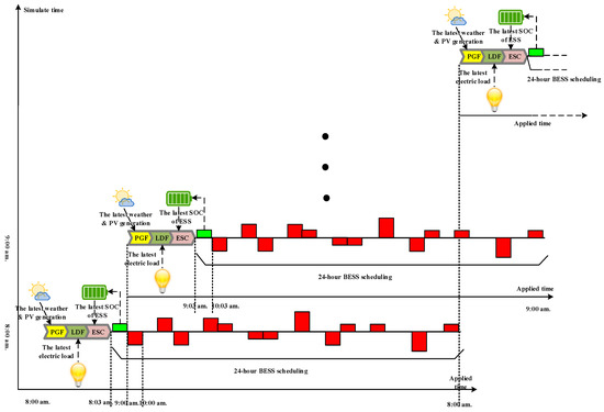
Figure 1.
Schematics of the rolling-horizon-based battery energy storage system (BESS) scheduling.
2.1. Mixed Integer Linear Programming Based Formulation
As mentioned above, the objective function of BESS scheduling is to minimize the total running cost , including the energy cost, demand charge, and the battery-wear-cost. The objective function can be formulated as follows:
where T is the rolling time horizon, which is selected to be 24 h. is the TOU price at time t. and represent the maximum and minimum SOC limits, respectively. and are the efficiency of discharge and charge, respectively. In Equation (1), the first part represents the energy cost, billed at the price of TOU. Because the electricity bill will be charged based on the measurement at the point of common coupling (PCC), the scheduled net flow of PCC considering BESS scheduling can be defined as:
where and are the forecasted load and solar generation at time t, respectively, and and represent the discharge and charge power.
The second part represents the battery wear-cost. The wear-cost model of BESS is complicated because it depends on many factors, such as discharge rate, SOC, and depth of discharge (DOD), among which DOD is the most widely considered [15]. Due to the strict linear limit of MILP, the nonlinear relationship between DOD and its life cycle is linearized by a simplified linear wear cost model (SLBWM). In this model, wear-cost can be calculated based on the equivalent full discharge cycle at the price of the unit wear-cost price of each discharge cycle. The unit wear-cost price of each discharge cycle is obtained by dividing the battery installation cost by the available cycle number () for the corresponding DOD value. is the rated capacity of BESS. To obtain more accurate results, the wear-costs calculated by SLBWM with different DOD values are compared with the cost calculated using the rain-flow algorithm [16,17]. The DOD value when the wear-cost values calculated by the two methods best matches is selected as the representative DOD value. At the current market price of BESS, the operation cost and the life time of BESS are important concerns to the customers to optimize the return on their investment. Therefore, the wear-cost of BESS is an important issue in many studies [15,18]. However, as technology matures, and markets expand, the price of BESS will decrease and the lifetime may not heavily depend on the discharge cycle. If the battery wear-cost is insignificant or negligible in the total running cost, the weight parameter can be set to a smaller value or zero.
The third part of the objective function is about the demand charge, which is billed at the penalty price () for the improper usage of power when the maximum net flow during any measured period exceeds the contract power (). The integer variable I is introduced to indicate whether the penalty is applied, as given by:
To calculate the demand charge, the power flow at PCC is measured periodically. To calculate the exact demand charge and generate an optimal scheduling considering the contract demand, the maximum net flow at PCC should be formulated into a problem and recorded. This requires additional formulation as follows:
- Introduce binary variables , where = 1 if is the maximum value, otherwise it is 0.
- Obtain the upper and lower bounds of the net flow at time and reformulate MILP:where is the maximum value of the net flow upper limits during the time horizon T.
SOC of BESS at time is constrained as follows:
where SOC of BESS at any time t can be calculated by the following equation:
Moreover, the instantaneous discharge/charge power of BESS depends on the capacity of PCS. The constraint for this physical limit is given as follows:
where is the rated power capacity of PCS, is a binary variable introduced to prevent the charge and discharge from occurring simultaneously:
The proposed MILP-based optimal scheduling problem is implemented and solved in a MATLAB (R2017a, MathWorks, Natick, MA, USA) environment.
2.2. Target SOC Value Assignment Method
For the economic and reliable operation of a microgrid, it is very important to keep the SOC value of BESS within the appropriate range. Therefore, when scheduling BESS, the SOC value of the last hour must be carefully selected and included as a constraint, as given by Equation (13):
In day-ahead-based scheduling, the value of can be a fixed value because the start and end time of scheduling are always the same every day, e.g., from 1 to 24 h. A reasonable value of is 50% or the average value of and . However, it is more complicated to determine the target SOC value in a rolling-horizon-based approach because it derives the scheduling every hour. One simple approach, proposed in [19], is to set the target SOC value at t = T the same as the current SOC value (), i.e., . Hereafter, this method will be referred to as the equivalent assignment method (EAM). It is based on the periodicity and is therefore suitable for use in rolling-horizon-based scheduling. However, in some situations EAM may not perform as well. For example, if the current SOC value is very low after an unusual discharge and the target SOC value is set as the same as the current value, BESS may not be charged enough to compensate for the subsequent high demand. On the contrary, if the current SOC is unusually high for some reason, an unnecessary charge schedule will be generated, which will lead to uneconomical operation.
To mitigate the aforementioned problem, a modified rule to set the target SOC value is proposed below in Equation (14):
This will be referred to as the flexible assignment method (FAM). The new rule copes with abnormal situations as well as reflecting the daily periodicity. The performance comparison between EAM and FAM will be presented in Section 4.
2.3. Confidence-Weight Method for Modifying Forecasted Load
In this part, we propose a confidence-weight method to modify the predicted load before it is inputted to the ESC program. The ARIMA model is adopted for load forecasting. The effectiveness of ARIMA-based forecasts has already been demonstrated in several studies [20,21]. However, one disadvantage of the ARIMA-model-based short-term forecast is the heavy dependence on the latest historical data. Electricity demand can be changed suddenly due to various unpredictable events, especially in a small-scale microgrid. Therefore, some temporary and fast-changing data can result in over- or under-estimation for the next 24-h forecast. In such a situation, the accuracy of BESS scheduling cannot be guaranteed. Therefore, to mitigate the effect of sudden load variations, the weighted average value of the predicted load data for the past 12 h will be used. The largest weight is given to the load value predicted at the present time, and the weight gradually decreases to the minimum value for the load predicted 12 h ago. The set of confidence weight parameters for the load at each time in the current 24-h forecast is also different. The equations for the confidence weight parameters calculation are given as follows:
where is (i − 1)th past-predicted load data for time t, is the weight parameter for the corresponding (i − 1)th past-forecasted load of time t. It should be normalized as follows:
In summary, the closer the time, the lower is the confidence of the past forecast; the farther the time, the higher is the dependence on the past forecast. Parameter a is a simple ratio that represents the declining speed of credibility for the following time t in the current forecast. As an example, the degree of dependence on the past-forecasted load data of the first predicted load at the current forecast will be dropped off at the speed of 100 times, i.e., is set to 100. The confidence weight parameters for each time are displayed in Figure 2.
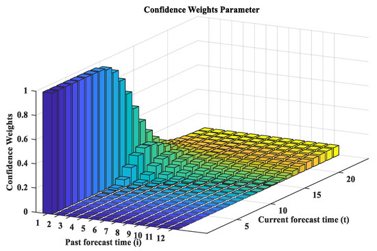
Figure 2.
Confidence weight parameters for the past 12-h forecast load.
3. Real Time Control Scheme for Handling Forecast Uncertainty
The performance of the BESS scheduling depends significantly on the accuracy of LDF and PGF. However, the forecast uncertainty is inevitable and cannot be ignored, especially for a small system like a microgrid. Therefore, to improve the performance of the microgrid operation, real-time control schemes (RTCSs) are required. In this section, a novel real-time control scheme is proposed and compared with the existing approach, where simply the mismatch between forecast and actual net load is compensated [10,11]. The above mentioned LDF, PGF, and ESC are embedded into a developed microgrid energy management system (MGEMS). To implement the real time control scheme, a new application program is added. Before the BESS operation command is sent to battery management system (BMS), RTCS modifies it considering the real time measurement of PV generation and load. The process including RTCS is illustrated in Figure 3.
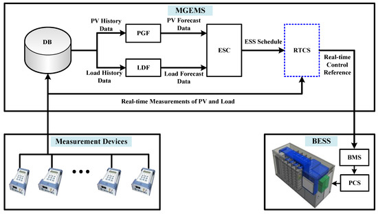
Figure 3.
Schematics of real-time control of BESS.
Without RTCS, BMS will receive the control command from ESC directly. It is the pure application of the optimal BESS scheduling result, without considering the real time variation of load conditions and battery state. For simplicity, the control scheme without RTCS is referred to as the pure schedule control scheme (PSCS).
3.1. RTCS1: Control to Maintain the PCC Net Flow as Scheduled
A straightforward real-time control method has been proposed in [10,11], and it will be referred to as RTCS1. The goal of RTCS1 is to keep the net flow at PCC as scheduled. Therefore, if the actual net load is different form the forecasted one, RTCS will modify the BESS control command. The adjusted real-time control command will recover the actual PCC net flow to be the same as the scheduled value unless BESS has no capability to support due to the limitations of the BESS capacity. Therefore, the real-control command can be calculated as follows:
where and are the real time measurement of the load and solar generation, respectively, and is the scheduled BESS operation reference at the corresponding time. is the required power for BESS to maintain the net flow at PCC as scheduled. If the SOC and PCS capacity limits of BESS are not exceeded, it will be the real-time control command. Otherwise, it should be adjusted again according to the limit values.
3.2. RTCS2: Intelligent Scheduling Decision Against Actual Situation
We propose a novel real-time control scheme, called RTCS2. When determining the real-time control command, RTCS2 considers not only the mismatch between the actual and forecasted net load but also many other factors, such as the current load level, scheduled value, current and expected SOC levels, etc. Considering that the penalty price is much higher than the TOU price, a common primary purpose of real-time control is peak-load reduction to avoid the demand charge. However, in some situations, maintaining the scheduled SOC level is more important for continuous operation. Therefore, an intelligent control decision is required to effectively reduce the demand charge induced by the sudden rising load and prevent an excessive SOC drop. The rules to determine the real-time control command according to the actual and forecasted net load will be explained in detail.
- When the actual net load is larger than the forecasted net load,
- (a)
- If the actual net load does not exceed the contract demand, BESS will be controlled as scheduled, unless the scheduled charging leads to a contract demand violation. If the scheduled charging is too large, it will be adjusted until the actual net flow is the same as the contract demand.
- (b)
- If the actual net load exceeds the contract demand, but the forecasted net load does not, BESS will be controlled to reduce the actual net flow to the contract demand. In other words, BESS will increase the discharge or decrease the charge compared to the schedule.
- (c)
- If both the actual and forecasted net load exceed the contract demand, the demand charge is unavoidable. In this case, in order not to raise the demand charge as well as to maintain the SOC within appropriate level, BESS will be controlled to keep the PCC net flow as scheduled.
Therefore, the real time control scheme in this condition can be summarized as follows:
- When the actual net load is less than the forecasted net load,
- (a)
- If BESS was scheduled to charge, the real-time command will be set the same as the scheduled reference. This control will not increase the net flow at PCC, as well as enough energy can be charged as scheduled for future operation.
- (b)
- If BESS was scheduled to discharge and no demand charge was expected, the real-time command can be calculated such that the PCC net flow is maintained as scheduled. However, if the calculated value is negative, the real-time command will be set to zero to operate BESS in stand-by instead of charging mode. In this condition, by reducing the discharge, the saved energy can be used for future operation.
- (c)
- If the demand charge was expected despite the scheduled discharge, BESS will be controlled to reduce the demand charge. However, in this situation, over-discharge exceeding the scheduled value is not allowed because it will lead to an excessive reduction of SOC.
The aforementioned control decisions in this condition can be summarized as follows:
where is the expected net flow of PCC in the scheduling, which is equivalent to the forecasted net load minus the scheduled BESS power. will be used as the real time control command if the physical limits of BESS are not violated; otherwise, the value should be adjusted in accordance with the limits.
4. Simulation Results and Analysis
The BESS scheduling and real-time control schemes, together with LDF and PGF, are tested with the data actually measured from the microgrid being built at the Chonnam National University (CNU) campus, South Korea. An illustration of the campus microgrid model is displayed in Figure 4. In this microgrid, a 250-kWh BESS with the same PCS capacity and a 50 kW PV are installed. Nearly half-a-year of load and PV generation profiles, used as input data for LDF and PGF, have been collected. Because the project is underway, BESS is not yet fully controlled by MGEMS. Therefore, the proposed methods are simulated offline using the real measured data. In other words, the PV and load forecasts and the BESS schedule are derived based on real measurement data; however, the control signal is not delivered to BESS. Instead, the behavior of BESS is simulated based on a mathematical model by considering the real characteristic parameters.
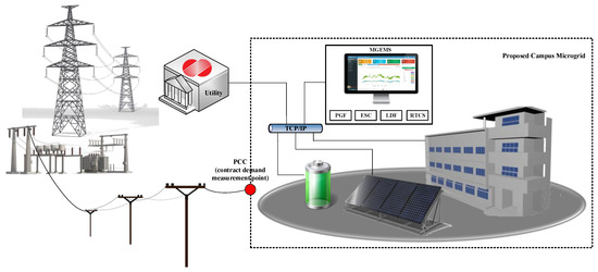
Figure 4.
Schematics of a campus microgrid model.
4.1. Improvement of LDF Performance by the Proposed Confidence Weight Parameter Method
As mentioned in Section 2.3, the major shortcoming of the ARIMA-based forecast program is the heavy dependence on the latest updated data. The forecast at the time of the peak demand or valley demand can result in an over- or under-estimation for the next 24-h forecast. The predicted data of each cycle in the rolling-horizon strategy should be modified before being used as the input to the ESC program. To demonstrate the effectiveness of the proposed modification method, numerous simulations were conducted and analyzed. The load data for the simulation were collected from the CNU microgrid from August to December 2017. As the load pattern during weekends is quite different from that during the week and the data classification for day types is not developed yet in LDF, only the weekday data are used in this simulation. Finally, the data of 79 days over 4 months are selected, excluding days with bad or missing data. Under the rolling-horizon strategy, 1 h is selected as the rolling cycle, which means that LDF will run nearly 1900 times during a 79-day continuous operation.
To verify the effectiveness of the proposed method, the mean absolute percentage error (MAPE) for the next 24-h is calculated for every rolling cycle as follows:
Figure 5 compares the cumulative distributions of MAPE(t) before and after the proposed method was applied. It is noteworthy that the proportion of cases with a MAPE of less than 4% increased by 14.4%, from 3.5% to 17.9%, by applying the proposed method. It proves that the overall accuracy of 24-h load forecast is substantially improved. Another important improvement with the method is that the cases with extremely high error have been reduced. For example, the cases with MAPE exceeding 20% decreased from 1.2% to 0.6%. Therefore, it is expected that the operation failure of BESS due to the forecast error will be greatly reduced. In the following simulation cases, we will use the load forecast after applying the proposed method.
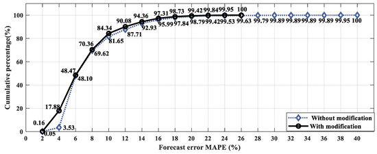
Figure 5.
Mean absolute percentage error (MAPE) cumulative distribution with and without modification.
4.2. Performance Comparison of Real Time Control Schemes for a Sample Case
The performance of the proposed rolling-horizon-strategy-based BESS scheduling and real time control scheme are simulated and demonstrated. The simulation is conducted with the conditions shown in Table 1.

Table 1.
Simulation parameters for battery energy storage system (BESS) scheduling and real-time control scheme (RTCS) for the sample case.
As described in the Section 2, the wear-cost of BESS can be weighted by adjusting the parameter Bw. In the following simulation, the weight factor is selected to be 1.0. The TOU price is obtained from the utility and plotted in Figure 6.
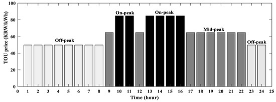
Figure 6.
Time of use price used in the simulation.
In this part, the performance of different real-time control schemes will be analyzed with sample 48-h operation data. The input data and simulation results are displayed in Figure 7, Figure 8 and Figure 9. Figure 7a shows the forecasted and actual net load data. The net load at peak hours exceeds the contract demand, which would lead to a demand charge without proper BESS operation. Figure 7b shows the BESS operation under PSCS, where no real-time control is applied. In this case, an operation schedule of BESS was provided based on the forecast information. For example, the discharges scheduled at 15:00 and 16:00 of the first day and at 17:00 of the second day were implemented to reduce the forecasted peak load below the contract demand, whereas the discharges at 10:00 and 11:00 of the second day were intended to save energy cost. The results of PSCS can be used as a reference to compare the performance of the two RTCSs.
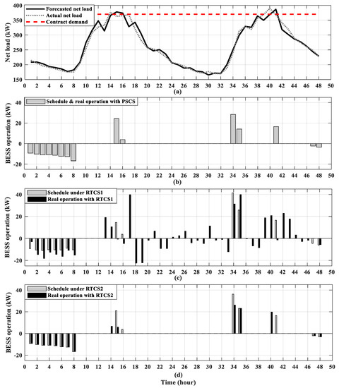
Figure 7.
Performance comparison between BESS control schemes. (a) forecasted and actual net load; (b) BESS operation under PSCS; (c) schedule and real operation of BESS under RTCS1; (d) schedule and real operation of BESS under RTCS2.
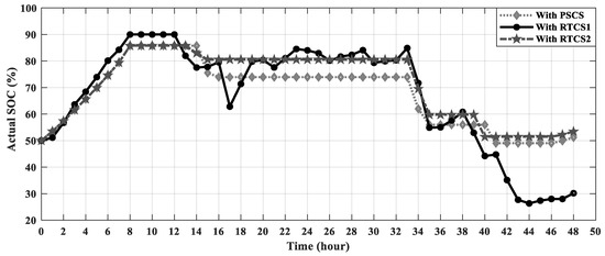
Figure 8.
Actual state of charge (SOC) profile with different BESS control schemes.
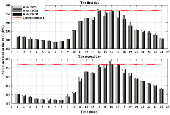
Figure 9.
Actual net flow at PCC considering BESS operation with different control schemes.
Figure 7c,d show the schedule and real operation of BESS under RTCS1 and RTCS2, respectively. The schedule results of the two RTCSs are similar to those of PSCS, but there are some differences, even though the load forecast data used in the three methods are the same. This is because the actual SOC values for each method are different at each rolling cycle. When the real-time control was applied, the BESS operation was different from the result of PSCS. The peak load exceeding the contract demand occurred one hour earlier than forecasted, and the discharge operation were performed accordingly, in both RTCS cases. This validates the effectiveness of RTCS against the forecast uncertainty. The operation results of RTCS1 and RTCS2 are quite different from each other. Most remarkably, RTCS1 shows frequent changes between charging and discharging. Because RTCS1 generates real-time control command to maintain the PCC net flow as scheduled, BESS has to operate even if there is a small mismatch between the forecasted and actual net load. This unnecessary operation can shorten the lifetime of BESS and increase the total cost. On the contrary, the real-time control command of RTCS2 is not changed from the optimal schedule unless it is inevitable.
Figure 8 displays the actual SOC profiles when the three different control schemes were applied. Obviously, SOC of BESS with RTCS1 fluctuates the most due to unnecessary charging and discharging operations. Moreover, it is also worth paying attention to the SOC value at the last hour after two days of operation. The last value of SOC with RTCS1 drops a lot due to the forecast error at 19:00 and 20:00 of the second day. This could adversely affect the next-day operation. For example, if an unexpectedly high demand occurs, RTCS1 may not be able to cope with this situation due to insufficient BESS capacity. However, such situations could be mitigated with RTCS2. An unnecessary discharge around 19:00 and 20:00 of the second day can be avoided. Thus SOC can be maintained at an appropriate value such that BESS can prepare well for future operations.
Figure 9 shows the actual net flows at PCC, after operation with the three control schemes. With PSCS, the net flows at 14:00 of the first day and 16:00 of the second day, when the actual peak demands occur, exceed the contract demand. Consequently, a demand charge was billed even though the BESS capacity is sufficient. In other words, the forecast uncertainty cannot be solved with the predetermined schedule-based operation. With RTCS1 and RTCS2, the PCC net flow at peak hours can be kept below the contract demand with an appropriate real-time control. Therefore, the demand charge, which was imposed unnecessarily with PSCS, can be avoided. The total operation cost for the two-day operation were 995,901, 862,939, and 843,825 Korean Won (KRW) with PSCS, RTCS1, and RTCS2, respectively. The cost are equivalent to $931, $806, and $789. The cost saving of the RTCSs compared to PSCS comes mainly from the demand charge. The BESS wear-cost were calculated to be 15,679, 37,579, and 14,755 KRW ($15, $35, and $14), respectively. The unnecessary frequent operation of RTCS1 results in a higher cost than RTCS2. Considering that the energy stored in BESS at the last hour was different, the cost saving of RTCS2 compared to RTCS1 would be even higher.
4.3. Performance Evaluation of the Proposed RTCS and Target SOC Assignment Method through Continuous Operation
In the previous simulation study, the performance of PSCS and the RTCSs were analyzed and compared through a sample case. However, the effectiveness and validity of the proposed methods should be further confirmed through a long-term operation of a microgrid considering various daily operating conditions. The same load data of 79 days, used in Section 4.1, were used in this continuous operation test. To present the comparison of the performance more clearly, the contract demand was set a little lower than the actual value. Consequently, the PCC net flow exceeded the contract demand for 35 days out of 79 days without BESS operation. The performance of the two target SOC assignment methods, i.e., EAM and FAM, and three real-time control schemes, i.e., PSCS, RTCS1, and RTCS2, were compared. For these six simulation scenarios, the total operation cost and the number of days when contract demand was violated were calculated. If the net load can be perfectly forecasted, the optimal schedule-based operation will yield the best performance. Therefore, the operation result adopting PSCS under the assumption of no forecast uncertainty is selected as a benchmark.
The simulation results of continuous operation under various scenarios are summarized in Table 2. The total operation cost of the benchmark scenario was minimal as expected. However, even with this optimal scheduling, the demand charge could not be avoided for 11 days. During those days, BESS was unable to support enough power due to its limited capacity, as the high load exceeding the contract demand continued for several hours. The optimal setting of the contract demand and battery sizing is an important topic for long-term operation, but it is beyond the scope of this paper. As shown in the last column of Table 2, RTCS1 and RTCS2 are effective in reducing the net flow at peak hours to avoid the demand charge, whereas PSCS could hardly handle this problem. In particular, RTCS2 with FAM shows the best performance among the six scenarios. In this scenario, the number of days of contract demand violation was reduced to 11 days, which is the same as for the benchmark case.
Table 2.
Simulation results of continuous operation under various scenarios.
The operation cost of all six scenarios were higher than that of the benchmark scenario, and the increase in the cost can be attributed to the forecast uncertainty. Figure 10 compares the increased cost due to the uncertainty. When PSCS was adopted, the cost increased by approximately 3,000,000 KRW ($2800), which is about 9% of the total cost. The cost increase was slightly reduced when the target SOC value was set by FAM. RTCS1 did not contribute to reducing the cost increase caused by the forecast uncertainty, although it could reduce the contract demand violation. It is speculated that unnecessary charging and discharging would result in uneconomical operation. RTCS2 could effectively reduce the cost due to uncertainty. When RTCS2 was applied combined with EAM and FAM, the cost increases were just 48% and 37% of that of PSCS, respectively. In summary, the proposed control scheme (RTCS2) could effectively reduce the cost due to uncertainty. Moreover, superior performance could be achieved with the proposed target SOC assignment method (FAM) compared to the existing one (EAM).
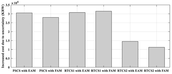
Figure 10.
Comparison of increased operation cost due to forecast uncertainty.
5. Conclusions
An MILP-based optimal scheduling of BESS for a microgrid operation was proposed, where the energy cost, demand charge, and battery wear-cost were considered in the objective function. To solve the problems arising when implementing the scheduling with the rolling-horizon strategy, two practical approaches were proposed. First, to improve the accuracy of the ARIMA-based load forecast, a confidence weight parameter method was applied. The performance was tested with the real measurement data of the campus microgrid. The results show that MAPE of a 24-h forecast period could be reduced considerably by applying the proposed method. Second, we proposed a new flexible target SOC assignment method. In addition, to solve the vulnerability of the schedule-based operation to the forecast uncertainty, a novel real-time control scheme has been proposed. The proposed RTCS could effectively reduce the cost caused by the uncertainty, as well as reduce the net flow at peak hours to avoid the demand charge. Especially, the performance of RTCS could be improved by combining with the proposed target SOC assignment method.
Author Contributions
H.-C.G. prepared the manuscript and implemented the theory and simulations. S.-J.A. and S.-Y.Y. supervised the study and discussed the results. J.-H.C. and H.-J.L. analyzed the simulation results and commented on the manuscript. All authors read and approved the final manuscript.
Funding
This work was supported by KEPCO Research Institute grant funded by Korea Electric Power Corporation (R16DA11).
Conflicts of Interest
The authors declare no conflict of interest.
References
- Markets and Markets Home Page. Available online: http://marketsandmarkets.com/PressReleases (accessed on 20 December 2017).
- Telaretti, E.; Ippolito, M.; Dusonchet, L. A Simple Operating Strategy of Small-Scale Battery Energy Storages for Energy Arbitrage under Dynamic Pricing Tariffs. Energies 2015, 9, 12–31. [Google Scholar] [CrossRef]
- Jeong, M.G.; Moon, S.I.; Hwang, P.I. Indirect Load Control for Energy Storage Systems Using Incentive Pricing under Time-of-Use Tariff. Energies 2016, 9, 558–577. [Google Scholar] [CrossRef]
- Kriett, O.P.; Salani, M. Optimal Control of a Residential Microgrid. Energy 2012, 42, 321–330. [Google Scholar] [CrossRef]
- Park, Y.G.; Kim, C.W.; Park, J.B. MILP-Based Dynamic Efficiency Scheduling Model of Battery Energy Storage Systems. J. Electr. Eng. Technol. 2016, 11, 1063–1069. [Google Scholar] [CrossRef]
- Jin, J.L.; Xu, Y.J. Optimal Storage Operation Under Demand Charge. IEEE Trans. Power Syst. 2017, 32, 795–808. [Google Scholar] [CrossRef]
- Zhang, Y.; Liu, B.; Zhang, T.; Guo, B. An Intelligent Control Strategy of Battery Energy Storage System for Microgrid Energy Management under Forecast Uncertainties. Int. J. Electrochem. 2014, 9, 4190–4204. [Google Scholar]
- Alharbi, W.; Raahemifar, K. Probabilistic Coordination of Microgrid Energy Resources Operation Considering Uncertainties. Electr. Power Syst. Res. 2015, 128, 1–10. [Google Scholar] [CrossRef]
- Yi, J.; Lyons, F.P.; Davison, J.P.; Wang, P.; Taylor, C.P. Robust Scheduling Scheme for Energy Storage to Facilitate High Penetration of Renewables. IEEE Trans. Sustain. Energy 2016, 7, 797–807. [Google Scholar] [CrossRef]
- Serpi, A.; Porru, M.; Damiano, A. An Optimal Power and Energy Management by Hybrid Energy Storage Systems in Microgrids. Energies 2017, 10, 1909–1929. [Google Scholar] [CrossRef]
- Huo, Y.; Jiang, P.; Zhu, Y.; Feng, S.; Wu, X. Optimal Real-Time Scheduling of Wind Integrated Power System Presented with Storage and Wind Forecast Uncertainties. Energies 2015, 8, 1080–1100. [Google Scholar] [CrossRef]
- Palma-Behnke, R.; Benavides, C.; Lanas, F.; Severino, B.; Reyes, L.; Llanos, J.; Sáez, D. A Microgrid Energy Management System Based on the Rolling Horizon Strategy. IEEE Trans. Smart Grid 2013, 4, 996–1006. [Google Scholar] [CrossRef]
- Solanki, V.B.; Raghurajan, A.; Bhattacharya, K.; Cañizares, A.C. Including Smart Loads for Optimal Demand Response in Integrated Energy Management Systems for Isolated Microgrids. IEEE Trans. Smart Grid 2017, 8, 1739–1748. [Google Scholar] [CrossRef]
- Xu, J.; Zhang, R. Real-Time Energy Storage Management for Renewable Integration in Microgrid: An Off-Line Optimization Approach. IEEE Trans. Smart Grid 2015, 6, 124–134. [Google Scholar]
- Chalise, S.; Sternhagen, J.; Hansen, M.T.; Tonkoski, R. Energy Management of Remote Microgrids Considering Battery Lifetime. Electr. J. 2016, 29, 1–10. [Google Scholar] [CrossRef]
- Musallam, M.; Johnson, M.C. An Efficient Implementation of the Rainflow Counting Algorithm for Life Consumption Estimation. IEEE Trans. Reliability 2012, 61, 978–986. [Google Scholar] [CrossRef]
- Li, J.; Gee, M.A.; Zhang, M.; Yuan, W. Analysis of Battery Lifetime Extension in a SMES-battery Hybrid Energy Storage System Using A Novel Battery Lifetime Model. Energy 2015, 86, 175–185. [Google Scholar] [CrossRef]
- Choi, Y.; Kim, H. Optimal Scheduling of Energy Storage System for Self-Sustainable Base Station Operation Considering Battery Wear-Out Cost. Energies 2016, 9, 462–480. [Google Scholar] [CrossRef]
- Heymann, B.; Bonnans, F.J.; Silva, F.; Lanas, F.; Jimenez, G. Continuous Optimal Control Approaches to Microgrid Energy Management. Energy Syst. 2018, 9, 59–77. [Google Scholar] [CrossRef]
- Kim, C.H.; Koo, B.G.; Park, J.H. Short-term Electric Load Forecasting Using Data Mining Technique. J. Electr. Eng. Technol. 2012, 7, 807–813. [Google Scholar] [CrossRef]
- Nataraja, C.; Gorawar, M.B.; Shilpa, G.N.; Shri Harsha, J. Short Term Load Forecasting Using Time Series Analysis: A Case Study for Karnataka, India. Int. J. Eng. Sci. Innov. Technol. 2012, 1, 45–53. [Google Scholar]
© 2018 by the authors. Licensee MDPI, Basel, Switzerland. This article is an open access article distributed under the terms and conditions of the Creative Commons Attribution (CC BY) license (http://creativecommons.org/licenses/by/4.0/).