Article

Risk Constrained Trading Strategies for Stochastic Generation with a Single-Price Balancing Market

Department of Electronic and Electrical Engineering, University of Strathclyde, Glasgow G1 1XQ, UK
Energies 2018, 11(6), 1345; https://doi.org/10.3390/en11061345
Submission received: 21 April 2018 / Revised: 10 May 2018 / Accepted: 23 May 2018 / Published: 25 May 2018
(This article belongs to the Section A: Sustainable Energy)

Abstract

:
Trading energy from wind and other forms of stochastic generation in competitive electricity markets is challenging due to the limited predictability of these resources. This paper examines the specific case of single-price balancing markets and derives risk-constrained strategies in a probabilistic framework, going beyond the trivial zero/max solution, which would have participants offer either zero or their maximum energy production based on a prediction of whether the system will be in net up- or down-regulation. The zero/max approach is unacceptable in reality as it exposes the participant to potentially huge imbalance charges, and would violate price taker assumption for a portfolio of significant size. Here, we propose several trading strategies that control risk by hedging against penalising balancing prices in favour of rewarding ones by contracting forecast generation plus some adjustment. These strategies are formulated in a probabilistic framework to address the presence of forecast uncertainty and asymmetric costs in balancing markets. A case study using data from the Great Britain electricity market is presented and it is shown that the proposed strategies are able to simultaneously increase revenue and reduce risk using risk-constrained strategies. Furthermore, the required forecasts of electricity prices and system length are produced using standard tools and widely available explanatory information and are found to have sufficient skill to increase revenue compared to not hedging.

1. Introduction

Since energy liberalisation in Europe, the US, and elsewhere, supply and demand have been matched by centralised operation of transmission systems using a combination of connected markets for energy and ancillary services [1]. Electricity markets were designed for dispatchable generators which are highly controllable and can therefore reliably deliver on production contracts agreed in advance. Production from stochastic generators, such as wind and solar, on the other hand, is uncertain and these generators rely on energy forecasts to participate economically in these markets; and, while high-quality forecasts are widely available and improving, they will never be perfect [2].
Much attention has been given to how stochastic generation can be integrated into electricity markets [3]. Strategies for their participation benefit from use of information about forecast uncertainty in order to deal with asymmetric penalties for over- or under-producing. Most of this work has focused on wind since this technology is more established, but the principals are transferable to other types of generation or smart grid actors such as aggregators [4,5]. Looking towards the future, new electricity market arrangements that facilitate the active participation of renewables in balancing markets are becoming a reality [6], and market designs that incorporate directly properties of stochastic generation by allowing probabilistic offers  [7], or risk-based decentralised operation [8], have been proposed.
Offer strategies for trading wind power in day-ahead markets are derived in [9], and, for dual-price balancing markets, the optimal quantile of a predictive distribution can be calculated based on forecasts of imbalance prices [10,11]. This analysis has been extended in [12,13] to include a recourse offer closer to the time of delivery, also for dual-price imbalance markets. Participation in an intraday power exchange (which facilitates anonymous bilateral trading) is considered in [14] by accepting available bids and offers which are deemed to improve the participant’s market position, although without a sophisticated offer strategy for the day-ahead market. Participation in US style markets with locational marginal pricing is considered in [15]. The strategic behaviour of wind power as a price-maker has also been studied [16,17].
Many of the trading strategies listed above and others are also presented in [3] covering both single- and dual-price balancing markets; however, risk-constrained strategies are only considered for dual-price markets. In fact, little attention has been given to the case of single-price imbalance markets despite such markets being operated in the US, Germany, the Netherlands and, since November 2015, the UK. In these markets, the arbitrage opportunity in the imbalance market dominates the trading strategies when maximising expected profit and leads to the unreasonable conclusion that stochastic producers should submit extreme bids (typically, and arbitrarily, constrained to zero and rated capacity of the producer) in the day-ahead market [18]. Furthermore, for a producer of any significant size, this approach would violate the “price taker” assumption in the imbalance market where traded volumes are much smaller than the day-ahead market. To address these issues, this paper explores risk-constrained strategies which enable stochastic producers to use this arbitrage opportunity to increasing profits while also reducing risk by hedging against penalising imbalance prices in favour of rewarding ones, rather than taking the extreme approach of attempting to maximise revenue from the imbalance market.
Participants in electricity markets require both power price forecast to inform their decision making, as the examples given above discuss. Electric utilities forecast prices from hours to months ahead in order to reduce risk or maximise profits, with day-ahead and intraday forecasts being critical for effective bidding strategies [1]. An extensive review of electricity price forecasting can be found in [19,20] and wind power forecasting in [21,22]. Results of the wind power and price forecasting tracks of the 2014 Global Energy Forecasting Competition in [23] give an overview of state-of-the-art practices. Electricity prices are driven fundamentally by supply and demand costs, and as such it is necessary to model these when making predictions [24,25,26]. Much attention has been given to short-term electricity prices, with familiar time-series models (ARX, ARIMA, etc.) being popular [27,28]. Forecasting balancing prices has received less attention but is considered in [29] and balancing volumes in [30], who use approaches based on ARIMA and exponential smoothing, respectively.
In this work, participation of stochastic generation in a day-ahead energy market coupled with a single-price balancing market is considered. Despite reputed difficulty in forecasting imbalance prices, it is shown that ARMAX time series models produce forecasts that are sufficient to use in trading strategies based on simple heuristics. A full probabilistic treatment based on probabilistic forecasts of all prices, generation and interdependencies is not considered here. It is observed that, in this situation, electricity market forecasts are of primary importance and that power forecasts are required only to apply risk-constraints. A secondary result is the observation of weak incentives for variable generation to provide accurate forecasts in this scenario, as also observed in [31]. The proposed strategies are based on taking a long or short position in order to manage asymmetric imbalance costs. Probabilistic forecasts of system length (sign of the net system imbalance) are required in addition to forecasts of day-ahead and balancing prices. Revenue maximisation and risk-constrained strategies are both derived, with only the latter requiring forecasts of power production.
An introduction to day-ahead and balancing markets is offered in Section 2. This is followed by the formulation of the offer strategy problem for single price balancing markets and possible solutions are presented in Section 3 which reveal the need for both price forecasts and a forecast of the probability that the system net imbalance will be negative (or positive). Issues with the trivial (and unsatisfactory) “bid zero or max” strategy are discussed, and risk-constrained alternatives are propsed. In Section 4, methods for producing the required probabilistic system length forecasts using logistic regression, and price forecast using ARMAX models, are introduced. A case study using real data form the UK is presented in Section 5. First, performance of the price and system length forecasts are compared to standard benchmarks before they are used to implement the trading strategies proposed in Section 3. The simple and risk-constrained trading strategies are then evaluated and their relative merits discussed. Finally, concluding remarks are made in Section 6.

2. Day-Ahead and Balancing Markets

Market structures can vary widely between regions but are typically made up of four main components: bi-lateral contracting between individual parties from days to years ahead of delivery, a day-ahead auction that determines the schedule for the activation of generators and large industrial consumers for the following day, an intraday market which allows participants to modify their position closer to delivery, and a balancing market utilised by the transmission system operator to balance supply and demand in real time and settle deviations from contracted volumes (imbalances) [32]. Additional markets may also exist for ancillary services such as frequency response, reserve power and provision of reactive power, and for financial products such as energy options and futures.
The most important markets for stochastic generators are the day-ahead and the balancing markets since the need to forecast generation makes trading further in advance challenging. Intraday markets enable participants to modify their position closer to gate closure, but often suffer from low liquidity, meaning that it is difficult for participants to find counter-parties to trade with. Day-ahead markets are typically double-blind auctions into which generators and consumers submit anonymous offers to generate and bids to consume certain volumes of energy at a price they are willing to pay or be paid. Supply and demand are compared and a market price is calculated for each period of the following day. This price is applied to all accepted bids and offers and is an important reference for intraday and balancing markets since it gives an indication of the marginal price of energy for a given period.
Balancing markets enable the transmission system operator to balance supply and demand and operate from gate closure to the point of delivery. The cost of balancing incurred by the system operator is recovered through payments by those who are out of balance. Prices are calculated based on either a single- or dual-pricing system. All participants in a single-price system resolve their imbalance at the same imbalance price, whereas in a dual-price system imbalances are settled at different prices depending on the sign of their imbalance. Balancing prices represent the cost to the system operator of increasing or decreasing net generation, and as such depend on whether the system has an overall energy surplus or deficit.
In a single-price balancing market, whether the single price is greater or less than the day-ahead price depends largely on the system length, i.e., whether the transmission system operator has had to increase or decrease net energy production during a given time period. If the system is short of energy, the balancing price will be greater than the day-ahead price to reflect the utilisation of more expensive or flexible generators (or demand reduction), and the converse if the system is long. The effect of this is to penalise market participants who are out-of-balance in the same direction as the system, and to reward those who are helping the system by being out-of-balance in the opposite direction. This is different to the two-price system where imbalances contributing to the system imbalance are penalised, and those helping are neither penalised nor rewarded.
The importance of system length forecasting is clear: being out-of-balance the wrong way invites a penalty, whereas being out-of-balance the right way is profitable. However, forecasting the system length prior to submitting offers into the day-ahead market is challenging and, since the penalties and rewards for a correct forecast are not systemic, warrants a probabilistic approach. In the following section, this problem is formulated and offer strategies for the day-ahead market are derived based on a probabilistic assessment of system length.

3. Problem Formulation

Here, we consider day-ahead offer strategies for a participant who is a price-taker in both day-ahead and balancing markets, and do not consider participation in intraday markets. For each settlement period t + k , a market participant will contract some volume of energy E t + k C at time t. The revenue R t + k for a participant contracting E t + k C but generating E t + k is given by
R t + k = π t + k C E t + k C T t + k C
where π t + k C is the contracted price for period t + k , and T t + k C is the cost associated with the energy imbalance d t + k = E t + k C E t + k . In a single-price balancing market, each participant must buy the volume of energy equal to their deficit, or sell the volume equal to their surplus, at the imbalance price. The imbalance price π t + k S is a function of the balancing actions relating to period t + k taken by the system operator to maintain the balance supply and demand in real time and is calculated at each settlement period. Revenue from the imbalance market T t + k C is given by
T t + k C = π t + k S d t + k .
It is useful to express a market participant’s revenue in terms of the actual energy they generate and their imbalance as follows
R t + k = π t + k C E t + k T t + k
from which it is clear that, to maximise revenue, balancing costs
T t + k = π t + k S π t + k C d t + k
should be minimised.
To reflect the dual-nature of the single imbalance price, we distinguish between the prices resulting from net up- or down-regulation, which corresponds to the sign of the system net imbalance volume (NIV). The NIV is positive when the system has an energy deficit (short), and negative when the system has an energy surplus (long). Equation (4) then becomes
T t + k = π t + k + π t + k C d t + k if NIV t + k > 0 π t + k π t + k C d t + k if NIV t + k 0 .
where π t + k + > π t + k C is the imbalance price is the system is short, and π t + k < π t + k C is the imbalance price if the system is long. The case NIV t + k = 0 is merged with NIV t + k < 0 for simplicity and without loss of generality since π t + k + = π t + k = π t + k C in that situation.
Assuming no participation in other markets or incentives to do otherwise, the aim of the market participant is to contract the volume of energy E t + k C that maximises revenue while managing risk.

3.1. Imbalance Minimisation

First, we consider the simplest strategy for risk management: minimise exposure to imbalance charges by contracting the forecast generation for each period in the day-ahead market. This approach reduces exposure to penalising imbalance prices, but also reduces exposure to rewarding prices in the case where the sign of the participant’s imbalance is the opposite that of the system. The bid in this case is given by
E t + k C = E ^ t + k | t ,
where E ^ t + k | t is a forecast of E t + k made at time t designed to minimise the mean absolute error. This strategy has the benefit of not requiring forecasts of market prices or system length.

3.2. Categorical Assessment of System Length

A participant’s revenue from the balancing market may be positive or negative depending on the sign of that participant’s imbalance, d t + k , and the sign of the system net imbalance volume, NIV t + k , as shown in Equation (5). Therefore, a strategic participant may attempt to predict the sign of NIV t + k to favourably influence the sign of their own imbalance by contacting more or less than they expect to produce.
Given a categorical forecast of system length (long or short), the revenue maximising volume to contract would be ± , according to Equation (5). This is of course nonsense and would violate market rules. Bounding this result by minimum and maximum offer volumes allowed by the market operator would also likely violate the price-taker assumption since large offers would influence the clearing price of the day-ahead market and NIV.
Any participant with sufficient power would have to consider their influence on the day-ahead price, NIV and the marginal price of balancing actions that the system operator would have to take, and the opinion of the market regulator. This situation is not considered here. We therefore proceed assuming that the capacity of the wind generators we consider is small relative to the magnitude of the NIV, and that the contracted volume is restricted to the range 0 E t + k C E max , where E max is maximum amount of energy the wind generator could deliver in a single settlement period.
If the sign of the NIV for period t + k is known, the optimal bid would be simply
E t + k C = 0 if NIV t + k > 0 E max if NIV t + k 0 .
A deterministic forecast of the sign of the NIV is required to implement this strategy, but note that no power forecast is needed. Note also that bidding only extremes leaves the participant exposed to potentially large losses if the sign of the NIV is forecast incorrectly.

3.3. Probabilistic Assessment of System Length

As imbalance prices in long and short periods are asymmetric about π C , it is desirable to formulate offer strategies from a  probabilistic perspective. Consider the energy generated during period t + k to be a random variable E t + k , and the probability at time t that the system will be short Pr t ( NIV t + k > 0 ) = ϕ t + k | t . We include the possibility that the NIV is exactly zero in the chance that the system is long without consequence, so Pr t ( NIV t + k 0 ) = 1 ϕ t + k | t . The subscripts t + k and t + k | t are dropped in the proceeding analysis to avoid notational clutter.
In this probabilistic framework, the expectation of the imbalance cost T is given by
E T = ϕ π + π C d + ( 1 ϕ ) π π C d
where d = E C E . Using the expectation operator E { · } , the bid that maximises expected revenue can now be calculated as
E ˜ C = argmin E C E T
= argmin E C ϕ ( π + π ) + π π C E d = argmin E C [ ϕ ( π + π ) + π π C
× E C E E ] .
Notice that the optimal bid depends only on the sign of the factor multiplying the expected imbalance. It is helpful to define the ratio
Φ = π C π π + π
and write the optimal bid as
E ˜ C = E max if ϕ < Φ 0 if ϕ Φ ,
where it is assumed that E C is bounded by 0 and E max . It is common for bids to be constrained by the capacity of the generator, although this constraint is somewhat arbitrary, especially in markets which allow non-physical merchant traders, for example. However, we proceed with it here to align with previous work and markets where such constraints do exist. If upper and lower limits were not imposed on E C , Equation (11) would return ± , which is clearly unrealistic. Furthermore, extending the range of E C too far beyond [ 0 , E max ] (or even far from the level of expected generation in the case of very large generators or portfolios) would violate our assumption that the participant is a price taker as large bids would influence the sign of the net imbalance and both the day-ahead and imbalance prices. The ratio in Equation (12) can be interpreted as a cost/loss ratio defining the critical probability at which it becomes economic to bid as if the system is expected to be long or short.
As the prices π C ,   π + and π are unknown at time t they must be forecast along with ϕ . Note, however, that there is no need to forecast the level of wind generation.

3.4. Risk Constrained Contracted Volume

Thus far, we have only considered revenue maximisation. Next, we consider a risk constrained approach for two main reasons: first, the risk associated with revenue maximisation is potentially large since imbalance prices are volatile and the strategies investigated so far require the participant to expose themselves to the largest imbalance possible; and, second, participants with potential market power may be able to participate in a similar way by hedging smaller volumes, and this should be done in an informed way.
In this section, alternative strategies are considered that restrict the size of the expected imbalance by adjusting the offer away from the forecast generation E ^ = E { E } to hedge against penalising imbalance prices. Three options are considered: an additive adjustment where the offer is equal to expected generation plus/minus some parameter, ν ; a multiplicative adjustment where the offer is equal to expected generation multiplied by some factor, 1 ± η ; and, finally, offering quantiles of probabilistic generation forecasts.

3.4.1. Additive Adjustment

In this strategy, the contracted energy for a given settlement period is the expected energy plus/minus a fixed adjustment. In effect, the capacity is partitioned into E ^ ν E max and 2 ν E max with the latter part traded using the probabilistic forecast of system length described in Section 3.3. The final offer bounded by 0 E C E max . This strategy can be written as
E C = min E max , E ^ + ν E max if ϕ < Φ max 0 , E ^ ν E max if ϕ Φ .
The choice of ν is a trade-off between maximising revenue and reducing exposure to imbalance charges.

3.4.2. Multiplicative Adjustment

Here, we consider a contracted volume proportional to the forecast generation. This strategy has the pleasing property that exposure to imbalance charges increases with expected generation, and therefore with expected revenue for a given period. Put differently, the participant is only exposed to risk when the expected revenue is already high, and is exposed to little risk when expected revenue is low. The contracted volume is equal to E ^ ± ( η × 100 ) % , bounded by zero and E max . The strategy given by
E C = min E max , ( 1 + η ) E ^ if ϕ < Φ max 0 , ( 1 η ) E ^ if ϕ Φ
where η 0 .

3.5. Quantile Offer

The additive and multiplicative strategies result in an imbalance d equal to the wind power forecast error, E ^ E , plus or minus an adjustment, the aim being to increase the likelihood that this term is either positive of negative, depending on the values of ϕ and Φ . Probabilistic forecasts provide information about forecast uncertainty and this information can be used to choose E C so that the probability of d > 0 has a particular value.
The predictive distribution of E can be described by a set of quantiles { q α , α [ 0 , 1 ] } where
Pr E < q α = α .
Writing this in terms of d and E C gives Pr d < q α E C = α . Therefore, the contracted volume E C which results in a probability α of d being negative is given by the quantile q α . This strategy is written as
E C = q α if ϕ < Φ q 1 α if ϕ Φ
where α is the probability that the realisation of d has the desired sign. The value of α is chosen heuristically to trade-off between revenue and risk.
This approach is attractive because it explicitly models the uncertainty associated with forecast errors allowing this risk-factor to be controlled explicitly. It is also more elegant since it removes the need to impose bounds on offers, as quantiles are bounded by [ 0 , E max ] automatically.

4. Forecasting

To implement the strategies described above, forecasts of prices, generation and the system length are required. This section outlines the methods used to produce these forecasts in the case study that follows. These methods have been informed state-of-the-art practices but we make no claim that they are optimal for this application. It should be noted that imbalance price forecasting is particularly challenging and has received very little attention in the academic literature. Here, we are concerned with the development and viability of trading strategies using accessible forecasts and leave improvement in forecasting methodology to future work.

4.1. Probabilistic System Length Forecast

The probability that the system will be short, ϕ , is estimated using a logistic regression model, which is a form of Generalised Linear Model. This approach allows ϕ to be estimated conditional on some set of explanatory variables X , formally,
ϕ = Pr ( NIV > 0 | X ) .
The logistic regression model is given by
log ϕ 1 ϕ = β × X t + k
where the vector β contains the model parameters to be estimated. Solving for ϕ yields
ϕ = 1 1 + exp ( β × X t + k ) .
Explanatory variables are chosen from the wide range of power system and market data that are available to participants. In this work, the parameters β are determined by maximum likelihood estimation using R, specifically the function glm from the package stats [33].
For the purposes of benchmarking different strategies, we will later consider the simple strategy where E C is chosen simply on the basis of whether the system is expected to be long or short, e.g., based on a deterministic forecast of system length. For that purpose, deterministic system length forecasts are produced using the method described above but rounding ϕ 0.5 to 1, and ϕ < 0.5 to 0.

4.2. Price Forecasts

For the purpose of this study, we employ the popular ARMAX-type models for price forecasting [19]. A separate ARMAX model is fit for each settlement period and type of day to capture the different dependencies between price and exogenous variables in each situation. The time index τ is used to indicate the position of price π τ in a sequence of prices corresponding to the settlement period and day-type. This approach regresses the price at time on its past values at τ 1 ,…, τ p , the model error ϵ τ and k exogenous variables X k , τ corresponding to time τ . The model is written as
π τ = a 0 + ϵ τ + i = 1 p a i π τ i + j = 1 q b j ϵ τ j + k c k X k , τ
where a i are the autoregressive coefficients, b j are the moving average coefficients, and c k are the regression coefficients for the exogenous variables. The forecast of π τ is given by
π ^ τ = a 0 + i = 1 p a i π τ i + j = 1 q b j ϵ τ j + k c k X k , τ .
The parameters a i ,   b j and c k are determined by maximum likelihood expectation, assuming that ϵ τ are independent and normally distributed, and the model order ( p , q ) is selected by minimising the Akaike Information Criterion implemented using the R package forecast [34].

4.3. Wind Power Quantile Forecasts

Quantile forecasts for time t, q ^ α , t are given by the function, q ^ α , t = Q α ( θ t ) , of explanatory variables, θ t , that is the solution to the following optimisation problem
argmin Q α t max ( 1 α ) ( q ^ α , t y t ) , α ( y t q ^ α , t ) .
Here, gradient boosted machines are used to determine Q α for α = 0.01 , 0.05 ,   , 0.95 , 0.99 , inspired by the winning entry from the 2014 Global Energy Forecasting Competition using the R package gbm [35,36].

5. Case Study and Results

The performance of the proposed trading strategies was evaluated in a case study using historic data from the GB power system in the UK. There are two coupled auctions operated by APX and N2EX (Nordpool) which clear at the same price for each hour of the next day. The balancing market comprises half-hour settlement periods and is operated by the System Operator (SO) and Elexon. Anonymous bilateral trading is facilitated by an intraday power exchange, but participation in this market is not considered here. Following the end of each settlement period, the single balancing price is calculated based on actions taken by the SO. This price is the volume-weighted average of the most expensive 50 MWh of balancing actions taken relating to that period.
Electricity market data are available from Elexon who operate the data service for the GB balancing mechanism. The data we utilised in this study are day-ahead and balancing prices, plus day-ahead forecasts of load, national wind and solar generation, and generation margin at peak demand (predicted volume of positive balancing energy available at the time of peak demand). Half-hour resolution wind power and day-ahead power forecasts for five UK wind farm were provided by an anonymous GB wind farm operator and aggregated, since imbalances are calculated on an aggregate basis.
The period from 6 November 2015 to 6 May 2016 was used in this case study covering the first six months following the switch from a dual- to single-price balancing mechanism. All analyses were performed on a hold-out basis where a portion of the data were held-out and used for out-of-sample testing while models were fit to the remaining data. The offer strategies described above were implemented with benchmarks based on perfect and simple forecasts to demonstrate the relative value and limitations of each method.

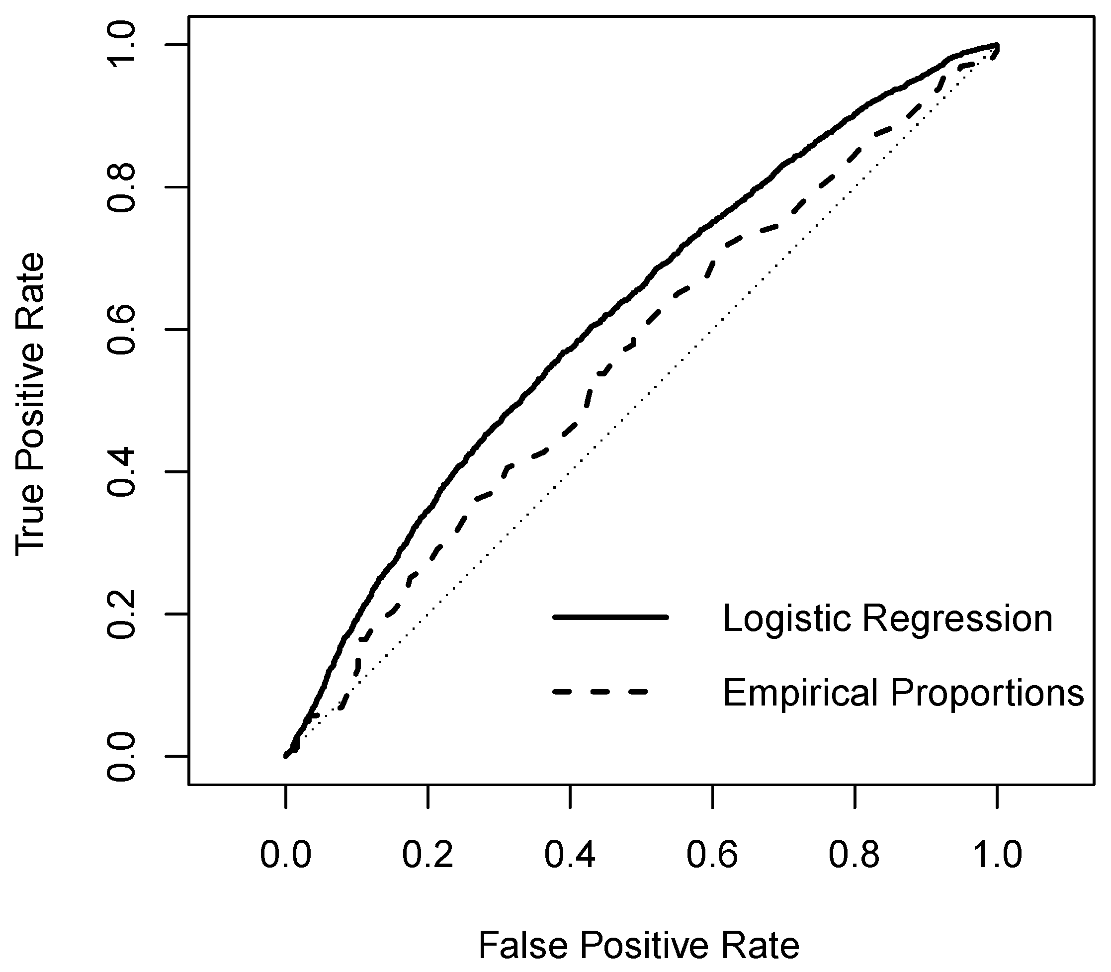
5.1. System Length Forecast and Evaluation

The performance of the probabilistic forecast of system length was first evaluated in terms of the Brier score and its decomposition. The Brier score is a proper scoring rule for probabilistic forecasts of binary events and is given by
Brier Score = 1 N i = 1 N ϕ i o i 2
where the observation o i = 1 if NIV i > 0 , and 0 otherwise [37]. The Brier score rewards both reliability and confidence. The best score achievable is 0 if either 0 or 1 is correctly forecast. Confident forecasts, i.e., those close to 0 or 1, are rewarded with a lower Brier score than cautions perditions, i.e., close to 0.5, if they are correct, and more heavily penalised if they are on the wrong side of 0.5.
The Brier score can be decomposed into reliability, resolution and uncertainty [38]. Reliability is a measure of how close the forecast probabilities are to the proportion of positive outcomes, resolution is a measure of how much the forecast probabilities vary from the climatic average, and uncertainty measures the inherent uncertainty of the event being forecast. Mathematically, these are given by
Reliability = 1 N k = 1 K n k ( ϕ k o ¯ k ) 2 ,
Resolution = 1 N k = 1 K n k ( o ¯ k o ¯ ) 2 ,
Uncertainty = o ¯ 1 o ¯ ,
where N is the total number of forecasts issued, K is the number of unique forecasts issued, and n k is the total number of times the kth unique forecast is issued. The terms o ¯ and o ¯ k are the mean outcome and the mean outcome conditional on the kth unique forecast being issued, respectively. Here, forecasts are grouped into 21 forecast bins centred on values from 0 to 1 in increments of 0.05.
A separate logistic regression model, Equation (20) is fit for each settlement period. Forecasts of load, wind generation, and generation margin at peak are included as explanatory variables for all periods, while forecast of solar generation are only used during hours of daylight, specifically Periods 12–41. Forecasts are produced out-of-sample for each day of the dataset using models trained on the all other data. As a benchmark, the historic proportion of occasion when each settlement period is short is used as a forecast and is referred to as empirical proportions when reporting results. The performance of these forecasts is tabulated in Table 1, along with the performance of the benchmark model.
The performance of binary forecasts such as these can also be evaluated by examining their relative operating characteristic (ROC) curves [39,40]. ROC curves depict the trade-off between true-positive and false-positive forecasts across the full range of predicted probabilities. Loosely, a more skilful forecast method is that with a higher true-positive and lower false-negative rate than the competing method. ROC curves for system length forecasts are presented in Figure 1, which illustrates that forecasts produced by logistic regression consistently outperform the benchmark.

5.2. Price Forecast Evaluation

The exogenous variables available for price forecasting are the same as those used in the logistic regression for system length forecasting, namely day-ahead forecasts of load, wind, solar, and generation margin. Data are grouped into three day-types: weekdays, weekends, and holidays. It should be noted that, because the day-ahead market requires offers to be submitted before 11:00 a.m., balancing prices for times later than this will not be available as input to the forecast of balancing prices for the next day. For this reason, two-step-ahead forecasts of balancing prices for periods after 10:00 a.m. are used, to allow for delays in the 10:00–10:30 a.m. and 10:30–11:00 a.m. balancing prices becoming available.
Models of order (1,1) and (2,1) are most common and account for over 25% of the models fit. Results are presented in terms of the critical probability, Φ = π C π π + π , and evaluated in terms of root mean square error (RMSE) and mean absolute error (MAE). These are given by
RMSE = 1 N t , k N Φ t + k Φ ^ t + k | t 2
and
MAE = 1 N t , k N Φ t + k Φ ^ t + k | t
where Φ ^ t + k | t is the forecast of Φ t + k made at time t, and N is the total number of samples.
The mean value of day-ahead and balancing prices from the same month and settlement period is used as a simple benchmark to asses the quality of the ARMAX forecasts. The MAE for the ARMAX and simple methods is 0.23 and 0.45, respectively; and the RMSE is 0.43 and 0.56, respectively. The ARMAX modelling approach clearly outperforms the simple method in terms of both error metrics. Forecasts from both methods were tested through implementation of the bidding strategies described in Section 3.2, Section 3.3 and Section 3.4 to quantify this improvement in monetary terms.

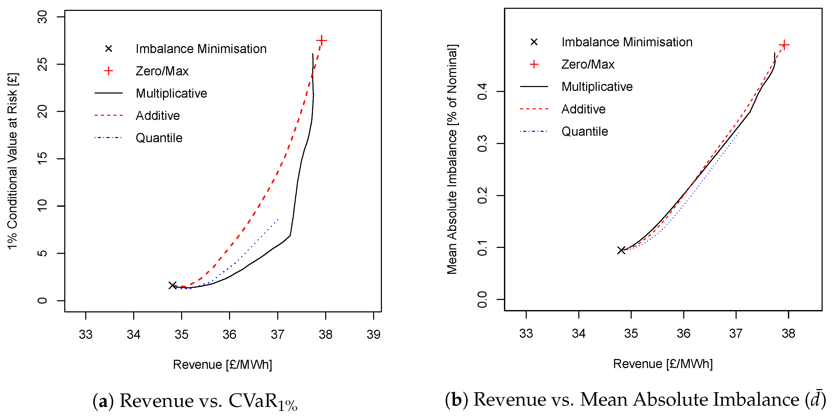
5.3. Offer Strategy Results

In this section, the revenues generated for the non-risk-constrained strategies described in Section 3.1, Section 3.2 and Section 3.3 are calculated using the half-hourly metered power from the aforementioned portfolio of five UK wind farms and the forecasts described above. These results are tabulated in Table 2 along with revenues derived from perfect and simple benchmark forecasts for comparison. The strategy based on a probabilistic assessment of system length is implemented for both the forecast methodology described in Section 4.1 and the empirical proportions (historic proportions for a given settlement period), which is used as a benchmark in Section 5.1. Only revenues from wholesale (day-ahead and balancing) markets are presented; any additional income from subsidies or other incentive schemes is not included, neither are the costs associated with securing access to the transmission system or electricity market membership.
These results indicate that strategies based on exploiting favourable imbalance prices and a probabilistic forecast of system length can generate more revenue than attempting to minimise imbalance volumes. In fact, even when contracting forecast energy production in the day-ahed market in order to minimise imbalance volumes, imbalances that result from imperfect generation forecasts generate positive revenue, on average. Trading based on a perfect generation forecasts resulted in the portfolio receiving £0.09/MWh less than the mean day-ahead price for the energy it generated due to negative correlation between wind power production and the day-ahead price, whereas imbalances caused by forecast errors resulted in receiving £0.06/MWh greater than the average price.
The strategy based on a deterministic forecast of system length only out performs trading forecast generation in the case of perfect foresight of system length as a result of the asymmetry between π + π C and π C π . When the system is long, the average value of π C π is £9.33/MWh, whereas when the system is short the average value of π + π C is £22.98/MWh. By trading based on a deterministic forecast of system length (i.e., on whether ϕ > 50 % ), the participant is exposed to an equal chance of a large loss or a small profit, on average, which results in a loss.
Strategies based on forecasting the critical probability Φ and probability of the system being long/short address this issue by hedging towards rewarding imbalance prices only when this is expected to yield positive revenue from the balancing market. The average value of Φ was 36.3% based on price forecasts indicating that, in general, the participant only positions themselves short if they are sufficiently confident (63.7%, on average) that the system will be long, effectively hedging away from the possibility of being short at the same time as the system is also short and having to “buy back” energy at a high price. The converse is also true: the participant prefers to risk long rather than short as the penalty when the systems is also long is small, but the reward when the system is short is large. The probabilistic forecast of system length based on logistic regression generates more revenue than that based on empirical proportions using simple price forecasts; however, the converse is true when using the advanced price forecasts, despite the logistic model having superior predictive performance. All strategies perform best when coupled with advanced rather than simple price forecasts. It is notable that perfect power forecasting does not increase revenue in the imbalance minimisation strategy.
Risk constrained strategies are evaluated in terms of revenue, the average size of imbalances, value at risk (VaR α ) and conditional value at risk (CVaR α ). The α % VaR is a threshold value such that the chance of the revenue being below that threshold is α % . Here, it is calculated as the α -percentile of the empirical distribution of settlement period revenue. Conditional value at risk, also called “expected shortfall”, is given by
CVaR α = 0 α VaR γ d γ
and gives the expected return in the worst α % of cases. Mean absolute imbalance, given by
d ˜ = mean | E t + k C E t + k | ,
is reported to compare the size of imbalance leveraged by each strategy.
Revenue, VaR 1 % , CVaR 1 % , and mean absolute imbalance are calculated for the three risk-constrained strategies described in Section 3.4. The probabilistic forecast of system length from the logistic model is used along with ARMAX forecasts of the prices. Plots of these results are presented in Figure 2a,b. Key results are tabulated in Table 3. Here, we examine results for the full range of possible parameters η , ν and α and examine the results ex-post, in practice, and user would be required to select one strategy and associated parameter value to trade on and update their selection adaptively over time to maintain the target level of risk-aversion.
When offer volume adjustments are small, all strategies successfully increase revenue with no increase in risk, and even a small decrease in risk in the case of the multiplicative and quantile strategies; however, all strategies tend towards the high-risk zero/max strategy for larger adjustments. This change in behaviour occurs at the highest revenue for the multiplicative strategy at the point where η = 1 , where the offer is either zero or 200% of expected generation. When η > 1 increasingly extreme short positions are taken while long positions are restricted since offers below zero are not possible. This asymmetry is a result of the imposition of maximum and minimum bids which is common in the academic literature but may not reflect market regulations in all cases and could be relaxed in future work.
The additive and quantile strategies, on the other hand, are able to take short positions regardless of expected generation resulting in more frequent and extreme short positions, and, therefore, more frequent losses and higher risk (VaR and CVaR). Since wind power generation is more likely to be close to zero than E max , the effect described above results in short positions being taken more frequently than long positions. This increases risk since short positions can result in negative revenue, whereas long positions can only result in reduced revenue, unless the balancing price is negative.
The multiplicative and quantile strategies with modest adjustments are clearly attractive options for participation in electricity markets with single-price balancing mechanisms as they have the effect of simultaneously increasing revenue and reducing risk. The benefits of these strategies in terms of realising a higher effective price per unit of energy generated are limited to participants of modest size as significant hedging at the day-ahead stage will exert influence on net imbalance volume and therefore revenues. In GB, for example, the mean absolute NIV for a 30 min settlement period is approximately 300 MWh with a standard deviation of 250 MWh. Small generators may be able to hedge a large portion of their capacity and thus increase their effective revenue-per-unit significantly, whereas large generators could only hedge a modest portion of their capacity else violate the price-taker assumption and as a result the impact on per-unit revenue would be small.

6. Conclusions

The stochastic nature of weather dependent renewables makes their participation in electricity markets challenging. In this paper, trading strategies for stochastic generation participating in electricity markets with single-price balancing mechanisms have been proposed and analysed. A new perspective on participation in single-price balancing markets based on a probabilistic treatment of system length has been presented. It is shown that by hedging against penalising imbalance prices, market participants both reduce imbalance charges and profit from increased exposure to favourable balancing prices. In the most extreme example, revenue is increased by almost 10% before considering any subsidy, however this requires the participant to leverage large imbalances that may be considered unacceptable by risk-averse generators, and poor practice by regulators. However, a more conservative risk-constrained approach can increase revenue while simultaneously decreasing risk. While the problem is formulated with the UK electricity market in mind, the principal of positioning oneself favourably in any day-ahead market is applicable to other problems where the cost of correcting that position is realised as a single price, be that a balancing price or some intraday contract.
Selecting offers for a day-ahead market coupled to a single-price balancing market has been formulated as a decision-making problem under uncertainty and solved in the first instance to maximise revenue, and in the second to constrain risk. In contrast to previous work, which has only considered categorical predictions of system length, predicting the probability of the system being long or short is proposed in a classical cost/loss type model, which also requires forecasts of imbalance prices. Conventional wisdom would suggest that basing strategies on forecasts of system length and imbalance prices is impractical due to the difficulty of predicting these quantities, and indeed it is shown here that a categorical prediction of system length was insufficient to increase revenue compared to simply trading forecast generation; however, it is also shown that there is sufficient skill in probabilistic system length forecasts and simple imbalance price forecasts to derive significant benefit using widely available explanatory data.
While imbalance price forecasting is certainly challenging, we have shown that familiar time series models are capable of producing forecast that are sufficient to be used in heuristic-based trading strategies. Improving the skill of system length and imbalance price forecasts would certainly improve the performance of the proposed strategies. Future work that considers electricity market participants’ risk aversion endogenously is encouraged but would require probabilistic forecasts of prices, generation and system length, including interdependencies. Indeed, the development of novel methods for probabilistic imbalance price forecasts are worthy of investigation in their own right. Furthermore, the limits of the price-taker assumption should be established, and the price-maker scenario studied.

Acknowledgments

The author acknowledges Elexon and an anonymous wind farm operator for the supply of data. This work was funded by an EPSRC Doctoral Prize, grant number EP/M508159/1.

Data Statement

The GB electricity market data used in this study are freely available from www.elexonportal.co.uk. Wind power production and forecast data are the property of an anonymous wind farm operator and are bound by a non-disclosure agreement.

Conflicts of Interest

The author declares no conflict of interest. The founding sponsors had no role in the design of the study; in the collection, analyses, or interpretation of data; in the writing of the manuscript, and in the decision to publish the results.

Nomenclature

R t + k Revenue from settlement period t + k
T t + k Imbalance cost in settlement period t + k
x ^ t + k | t Forecast of x t + k made at time t
E · Expectation operator
E t + k C Contracted volume for settlement period t + k
E t + k Actual energy delivered in settlement period t + k
d t + k Market participant’s imbalance E t + k C E t + k
d ¯ Mean absolute imbalance volume
E max Maximum deliverable volume in any single settlement period
π t + k C Price at which E t + k C is contracted
π t + k S Imbalance price
π t + k + Imbalance price during periods of net up-regulation
π t + k Imbalance price during periods of net down-regulation
NIV t + k Net Imbalance Volume for settlement period t + k ; a positive NIV is associated with up-regulation (‘the system is short’), negative NIV is associated with down-regulation (‘the system is long’)
ϕ t + k Probability that the system will be short, P ( NIV t + k > 0 )
Φ The ratio π C π π + π
q α The α -quantile forecast of energy production
ν , η , α Parameters of the additive, multiplicative and quantile trading strategies, respectively

References

  1. Edwards, D.W. Energy Trading and Investing: Trading, Risk Management and Structuring Deals in the Energy Market; McGraw-Hill: New York, NY, USA, 2009. [Google Scholar]
  2. Bessa, R.; Möhrlen, C.; Fundel, V.; Siefert, M.; Browell, J.; Haglund El Gaidi, S.; Hodge, B.M.; Cali, U.; Kariniotakis, G. Towards Improved Understanding of the Applicability of Uncertainty Forecasts in the Electric Power Industry. Energies 2017, 10, 1402. [Google Scholar] [CrossRef]
  3. Morales, J.; Conejo, A.; Madsen, H.; Pinson, P.; Zugno, M. Integrating Renewable in Electricity Markets; Springer: Heidelberg/Berlin, Germany, 2014. [Google Scholar]
  4. Pei, W.; Du, Y.; Deng, W.; Sheng, K.; Xiao, H.; Qu, H. Optimal Bidding Strategy and Intramarket Mechanism of Microgrid Aggregator in Real-Time Balancing Market. IEEE Trans. Ind. Inf. 2016, 12, 587–596. [Google Scholar] [CrossRef]
  5. Heydarian-Forushani, E.; Moghaddam, M.P.; Sheikh-El-Eslami, M.K.; Shafie-khah, M.; Catalão, J.P.S. Risk-Constrained Offering Strategy of Wind Power Producers Considering Intraday Demand Response Exchange. IEEE Trans. Sustain. Energy 2014, 5, 1036–1047. [Google Scholar] [CrossRef]
  6. Fernandes, C.; Frías, P.; Reneses, J. Participation of intermittent renewable generators in balancing mechanisms: A closer look into the Spanish market design. Renew. Energy 2016, 89, 305–316. [Google Scholar] [CrossRef]
  7. Papakonstantinou, A.; Pinson, P. Information Uncertainty in Electricity Markets: Introducing Probabilistic Offers. IEEE Power Engi. Lett. 2016, 31, 5202–5203. [Google Scholar] [CrossRef]
  8. Bahrami, S.; Amini, M.H. A decentralized trading algorithm for an electricity market with generation uncertainty. Appl. Energy 2018, 218, 520–532. [Google Scholar] [CrossRef]
  9. Bathurst, G.; Weatherill, J.; Strbac, G. Trading wind generation in short term energy markets. IEEE Trans. Power Syst. 2002, 17, 782–789. [Google Scholar] [CrossRef]
  10. Bremnes, J.B. Probabilistic Wind Power Forecasts Using Local Quantile Regression. Wind Energy 2004, 7, 47–54. [Google Scholar] [CrossRef]
  11. Pinson, P.; Chevallier, C.; Kariniotakis, G. Trading wind generation from short-term probabilistic forecasts of wind power. IEEE Trans. Power Syst. 2007, 22, 1148–1156. [Google Scholar] [CrossRef] [Green Version]
  12. Bitar, E.; Rajagopal, R.; Khargonekar, P.; Poolla, K.; Varaiya, P. Bringing Wind Energy to Market. IEEE Trans. Power Syst. 2012, 27, 1225–1235. [Google Scholar] [CrossRef]
  13. Morales, J.M.; Conejo, A.J.; Pérez-Ruiz, J. Short-term trading for a wind power producer. IEEE Trans. Power Syst. 2010, 25, 554–564. [Google Scholar] [CrossRef]
  14. Skajaa, A.; Edlund, K.; Morales, J.M. Intraday Trading of Wind Energy. IEEE Trans. Power Syst. 2015, 30, 3181–3189. [Google Scholar] [CrossRef]
  15. Botterud, A.; Zhou, Z.; Wang, J.; Bessa, R.J.; Keko, H.; Sumaili, J.; Miranda, V. Wind Power Trading Under Uncertainty in LMP Markets. IEEE Trans. Power Syst. 2012, 27, 894–903. [Google Scholar] [CrossRef]
  16. Zugno, M.; Morales, J.M.; Pinson, P.; Madsen, H. Pool Strategy of a Price-Maker Wind Power Producer. IEEE Trans. Power Syst. 2013, 28, 3440–3450. [Google Scholar] [CrossRef]
  17. Delikaraoglou, S.; Papakonstantinou, A.; Ordoudis, C.; Pinson, P. Price-maker wind power producer participating in a joint day-ahead and real-time market. In Proceedings of the 12th International Conference on the European Energy Market, Lisbon, Portugal, 19–22 May 2015; pp. 1–5. [Google Scholar]
  18. Mazzi, N.; Pinson, P. 10—Wind power in electricity markets and the value of forecasting. In Renewable Energy Forecasting; Kariniotakis, G., Ed.; Woodhead Publishing Series in Energy; Woodhead Publishing: Sawston, UK, 2017; pp. 259–278. [Google Scholar]
  19. Weron, R. Electricity price forecasting: A review of the state-of-the-art with a look into the future. Int. J. Forecast. 2014, 30, 1030–1081. [Google Scholar] [CrossRef]
  20. Nowotarski, J.; Weron, R. Recent advances in electricity price forecasting: A review of probabilistic forecasting. Renew. Sustain. Energy Rev. 2018, 81, 1548–1568. [Google Scholar] [CrossRef]
  21. Giebel, G.; Brownsword, R.; Kariniotakis, G.; Denhard, M.; Draxl, C. The State-Of-The-Art in Short-Term Prediction of Wind Power: A Literature Overview, 2nd ed.; ANEMOS.plus; European Commission: Brussels, Belgium, 2011. [Google Scholar]
  22. Foley, A.M.; Leahy, P.G.; Marvuglia, A.; McKeogh, E.J. Current methods and advances in forecasting of wind power generation. Renew. Energy 2012, 37, 1–8. [Google Scholar] [CrossRef] [Green Version]
  23. Hong, T.; Pinson, P.; Fan, S.; Zareipour, H.; Troccoli, A.; Hyndman, R.J. Probabilistic energy forecasting: Global Energy Forecasting Competition 2014 and beyond. Int. J. Forecast. 2016, 32, 896–913. [Google Scholar] [CrossRef] [Green Version]
  24. Karakatsani, N.V.; Bunn, D.W. Forecasting electricity prices: The impact of fundamentals and time-varying coefficients. Int. J. Forecast. 2008, 24, 764–785. [Google Scholar] [CrossRef]
  25. Brijs, T.; Vos, K.D.; Jonghe, C.D.; Belmans, R. Statistical analysis of negative prices in European balancing markets. Renew. Energy 2015, 80, 53–60. [Google Scholar] [CrossRef]
  26. Andrade, J.; Filipe, J.; Reis, M.; Bessa, R. Probabilistic Price Forecasting for Day-Ahead and Intraday Markets: Beyond the Statistical Model. Sustainability 2017, 9, 1990. [Google Scholar] [CrossRef]
  27. Amini, M.H.; Kargarian, A.; Karabasoglu, O. ARIMA-based decoupled time series forecasting of electric vehicle charging demand for stochastic power system operation. Electr. Power Syst. Res. 2016, 140, 378–390. [Google Scholar] [CrossRef]
  28. Ziel, F.; Steinert, R.; Husmann, S. Efficient Modeling and Forecasting of the Electricity Spot Price. Energy Econ. 2015, 47, 98–111. [Google Scholar] [CrossRef]
  29. Olsson, M.; Söder, L. Modeling real-time balancing power market prices using combined SARIMA and Markov processes. IEEE Trans. Power Syst. 2008, 23, 443–450. [Google Scholar] [CrossRef]
  30. Jónsson, T.; Pinson, P.; Nielsen, H.A.; Madsen, H. Exponential Smoothing Approaches for Prediction in Real-Time Electricity Markets. Energies 2014, 7, 3710–3732. [Google Scholar] [CrossRef] [Green Version]
  31. Hirth, L.; Ziegenhagen, I. Balancing power and variable renewables: Three links. Renew. Sustain. Energy Rev. 2015, 50, 1035–1051. [Google Scholar] [CrossRef]
  32. Harris, C. Electricity Markets: Pricing, Structures and Economics; Wiley Finance: Hoboken, NJ, USA, 2006. [Google Scholar]
  33. R Core Team. R: A Language and Environment for Statistical Computing; R Foundation for Statistical Computing: Vienna, Austria, 2016. [Google Scholar]
  34. Hyndman, R.; Khandakar, Y. Automatic time series forecasting: The forecast package for R. J. Stat. Softw. 2008, 26, 1–22. [Google Scholar]
  35. Landry, M.; Erlinger, T.P.; Patschke, D.; Varrichio, C. Probabilistic gradient boosting machines for GEFCom2014 wind forecasting. Int. J. Forecast. 2016, 32, 1061–1066. [Google Scholar] [CrossRef]
  36. Ridgeway, G.; Southworth, H. gbm: Generalized Boosted Regression Models, R Package Version 2.1; 2014. Available online: https://CRAN.R-project.org/package=gbm (accessed on 20 April 2018).
  37. Brier, G. Verification of Forecasts Expressed in Terms of Probability. Mon. Weather Rev. 1950, 78, 1–3. [Google Scholar] [CrossRef]
  38. Murphy, A.H. A new vector partition of the probability score. J. Appl. Meteorol. 1973, 12, 595–600. [Google Scholar] [CrossRef]
  39. Spackman, K.A. Signal detection theory: Valuable tools for evaluating inductive learning. In Proceedings of the Sixth International Workshop on Machine Learning, Ithaca, NY, USA, 26–27 June 1989; pp. 160–163. [Google Scholar]
  40. Fawcett, T. An introduction to ROC analysis. Patt. Recognit. Lett. 2006, 27, 861–874. [Google Scholar] [CrossRef]
Figure 1. Relative operator characteristic curves for system length forecasts. The diagonal line, False Positive Rate = True Positive Rate, illustrates the performance of a random forecast, e.g., a random forecast of 70% would be expected to correctly predict 70% of all positive outcomes, and falsely predict that 70% of negative outcomes would be positive.
Energies 11 01345 g001
Figure 2. Plots of revenue vs. risk and imbalance volume for the three risk-constrained strategies with parameter values spanning those listed in Table 3. Crosses indicate the results from the revenue-maximising (zero/max) and imbalance minimising strategies tabulated in Table 2.
Energies 11 01345 g002
Table 1. Brier scores for probabilistic system length forecasts. The uncertainty component of the Brier score is 0.2337 in both cases.
MethodBrier ScoreReliabilityResolution
Empirical Proportions0.23180.00010.0029
Logistic Regression0.22650.00300.0102
Table 2. Normalised revenue (£/MWh) using different trading strategies. For strategies marked * “Forecast Method” refers to the type of price forecast only. The mean day-ahead price during the test period was £34.75/MWh.
StrategyForecast Method
PerfectSimpleAdvanced
Minimise Imbalance34.66n/a 34.81
SL Forecast: Deterministic50.1633.2034.39
SL Forecast: Empirical Proportion * 41.7237.3237.75
SL Forecast: Logistic * 41.4336.2537.92
Table 3. Performance of the risk-constrained offer strategies. The case ν , η = 0 is equivalent to offering a volume equal to the wind power forecast (imbalance minimisation), the additive adjustment strategy with ν = 1 is equivalent to offering zero/max.
Additive Adjustment
ν RevenueVaR 1 % CVaR 1 % d ˜
034.810.551.619%
0.135.390.722.3013%
0.537.168.2215.3436%
137.9214.2327.5149%
Multiplicative Adjustment
η RevenueVaR 1 % CVaR 1 % d ˜
034.810.551.619%
0.135.020.431.3810%
0.536.020.822.6020%
137.262.576.8736%
537.7211.1319.7145%
1037.7314.1426.1147%
Quantile
α RevenueVaR 1 % CVaR 1 % d ˜
0.5534.900.451.3810%
0.6535.090.471.2710%
0.7535.320.451.4611%
0.9536.141.734.0720%
0.9937.053.758.7732%
Units:£/MWh£% of E max

