A New Perspective on Improving Hospital Energy Administration Based on Recurrence Interval Analysis

Abstract

Based on 15-min high-frequency power load data from a Chinese hospital, by adopting recurrence interval analysis, an attempt is made to provide a new perspective for improving hospital energy administration in electrical efficiency and safety. Initially, the definition of extreme fluctuation of the power load, as well as the recurrence interval, is given. Next, the stretched exponential distribution function is provided, which fits quite well with the probability density distribution of recurrence intervals. Then, tests on recurrence intervals, including scaling behavior and short-term and long-term memory effect are conducted. At last, a risk estimation method of VaR is proposed for hospital energy administrator to forecast risk probability. Results clearly indicate that the recurrence interval analysis (RIA) method works well on forecasting extreme power load fluctuation in hospital. However, there is no evidence to support the existence of the long-term memory effect of recurrence intervals, which means that hospital energy management plans have to be continuously fixed and updated with time. Some relevant applicant suggestions are provided for the energy administrator at the end of this paper.

1. Introduction

Hospitals all around the world consume an immense scale of energy in different ways and forms every year, which represent around 6% of the total energy consumption in the utility buildings sector [1]. As the public service sector, hospitals are almost functioning 24 h per day. Meanwhile, they are large building complexes incorporating kinds of medical instruments and facilities for heating, cooling, disinfect-purifying, infection controlling, administration, and so on. As a result, hospitals are two times, or even three times, more energy intensive than other institutional buildings, but less sensitive to the external climatic environment than most other building types. However, energy waste, as well as energy inefficiency, is quite severe in hospitals. In Europe, there is more than 20% of the consumed energy that is wasted in the hospital [2]. In the United States (US), it is declared by the Department of Energy that reducing hospital energy consumption by 20–30% is entirely feasible [3], while this number could soar to 45% in practice [4]. Therefore, the energy conservation and emission reduction in the hospital have become a hot topic of research.

In the context of the global economic depression, budget constraints are increasingly tighter for both public and private hospitals. When considering that most spending will go to healthcare facilitation, patient comfort, and staff wages [5], there is little space left from the budget to make a further investment on energy saving, upgrading, and reconstruction. It is a challenge for the administrator to reduce energy consumption without negatively impacting the high-quality comfort, service, productivity, and safety of the hospital. Given that the large-scale investment in energy-saving is not an option, it is better to concentrate on improving energy efficiency to reduce energy consumption and energy bill.

With the widespread use of the medical equipment as well as the sustainable improvement of the medical environment, hospitals consume more and more electricity resources [6]. Especially, in China, the electricity becomes the primary energy demand of the hospital, which occupies over 60% of the total energy consumption [7]. Hence, the energy management of hospital is more of improving electricity management in China.

Due to the time-of-use pricing system that is conducted by the power enterprise, shifting peak load (reducing electricity consumption during peak hours and increasing power consumption in off-peak time) is treated as an efficient way to promote electricity efficiency as well as to reduce power bill [8]. Facilities for power storage and ice thermal storage that are usually used at night to prevent electricity from reaching a peak in the daytime are widely applied in practice [9]. However, it has to be very careful to forecast the power consumption in the daytime, since either overestimation or underestimation will result in electricity waste, which would violate the intention. Therefore, as a management tool, power load data plays an indispensable role in forecasting electricity consumption [10,11].

Beside the electricity efficiency, the electrical safety of a hospital is another motivation of this study. With the advance of medical technology, the modern hospital is increasingly relying on medical equipment and instruments, a lot of which are large and high-power. As is known, it is probably well to generate shock load (It is a threat to the internal power system as the current can surge up to twenty times more than rated current at the start moment of running the high-power electrical appliance) when starting high-power machines. The shock could accelerate insulation aging and shorten the lifespan of electrical equipment and facilities. It is a threat to the hospital power system, which concerns not only the effect of diagnosis and treatment, but also patient’s life and death. The extreme positive power load fluctuation, indicating the synchronous start of massive high-power facilities and equipment, rarely occurs, but has serious consequences. For example, a fire that was caused by an electrical short circuit in a Korean hospital killed 37 people and injured 143 patients one 26 January 2018. A lounge heater was the last straw to the full load power line that caused the short circuit. The safe rated-capacity of the hospital cannot guarantee the electrical safety in each building. Therefore, the positive power load fluctuation is a signal of shock load in both risk probability and magnitude.

To the best knowledge of authors, the regression analysis method presuming the functional relationships of variables, are widely used in relevant researches since they can accurately quantify the tendency of power consumption [12,13,14]. However, the conventional practice of the regression method is to eliminate extreme values for the robustness of findings. Although the extreme volatility of power load happens rarely, it could lead to power crisis that would mess up the whole plan of energy management [15]. Therefore, the regression method may be a good choice for trend analysis, but it is incapable of forecasting extreme event. Besides that, time series models and the neural network (NN) models are also popular for electricity consumption forecast [16,17,18]. However, this kind of forecasting approaches may generate more errors as forecast values are used as inputs for next forecasts [19].

To forecast the risk probability of shock load as well as to avoid errors from presumable function and excessive round-off, the recurrence interval analysis (RIA) method is adopted in this paper. So far, this RIA method has proved to be effective in forecasting natural hazards, financial market volatility, and electricity consumption features in units of enterprise and office building [11,20,21,22,23]. Also, the introduction of high-frequent data is able to reflect the instantaneous fluctuation of power consumption, which does count for much more in hospital energy administration than daily data.

The rest of this paper is prepared, as follows. The detailed description of North Jiangsu hospital, as well as its electricity consumption characteristics, is given in Section 2. The method of recurrence interval analysis is introduced in Section 3, in which the descriptive statistics of the dataset is also presented. Section 4 focuses on the empirical study, where not only the distribution function and the scaling properties, but also memory effect and risk estimation are analyzed. Then, the conclusions of this paper as well as the relevant suggestions are delivered in Section 5.

2. Description of the Hospital

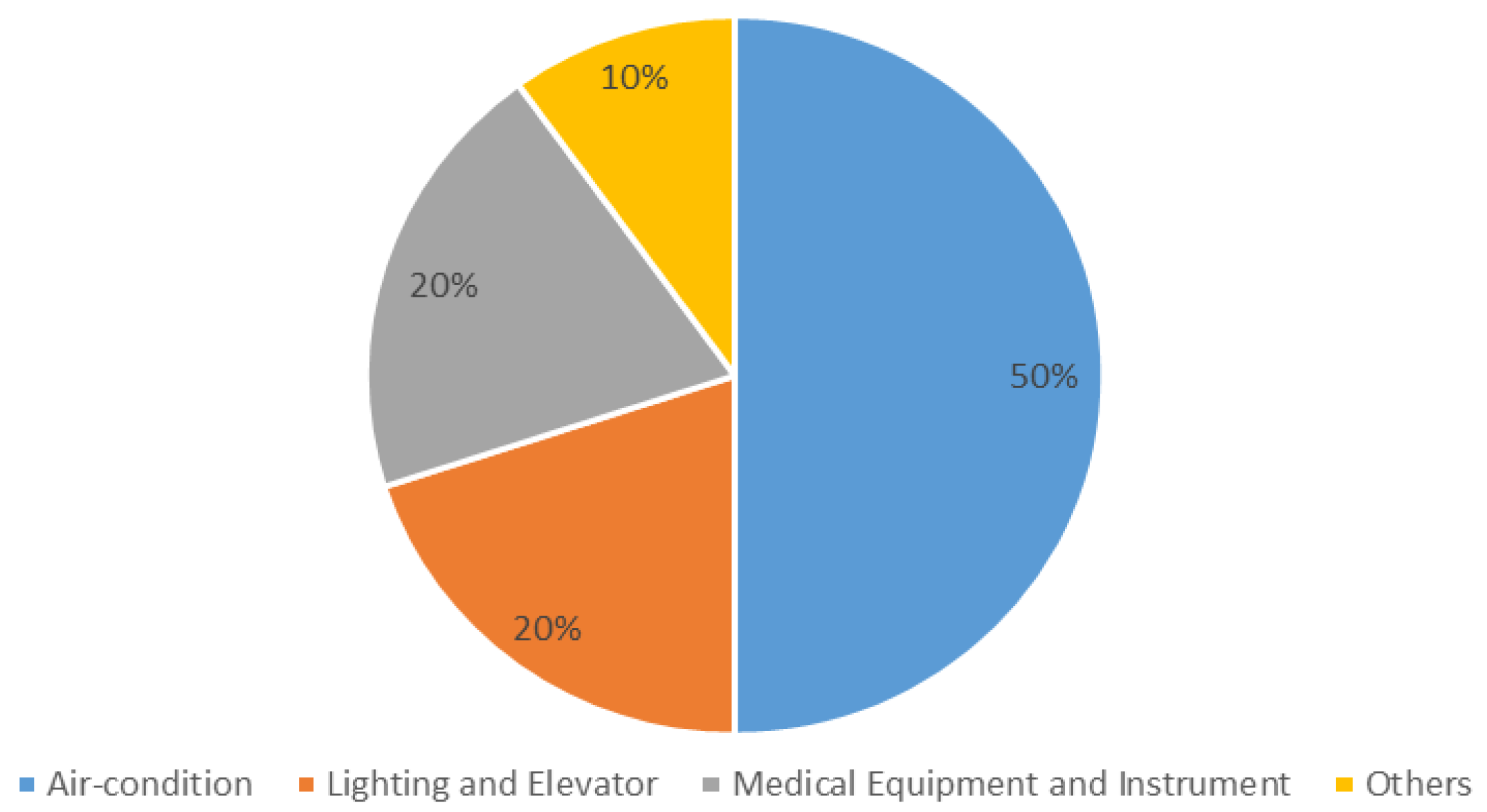
As a public hospital rating Level A in Grade III (according to a three-tier system hospitals in China are designed as Primary (Grade I), Secondary (Grade II), and Tertiary (Grade III). Further, based on the level of service, size, medical quality and so on, these three grades are subdivided into levels of A, B, and C. Hence, a hospital of Level A in Grade III is at the very top of nine levels), North Jiangsu hospital is located in a downtown area of the city of Yangzhou, Jiangsu Province, China. The energy consumption consists of electricity, water, steam, gas, petrol, diesel, and coal, in which power occupies more than 60% of the total energy demand. More specifically, 50% of the electricity consumption goes into the air-condition and the ventilating system, while lighting and elevators consume 20% of the electricity source, and so does the medical equipment and instruments [24], see Figure 1.

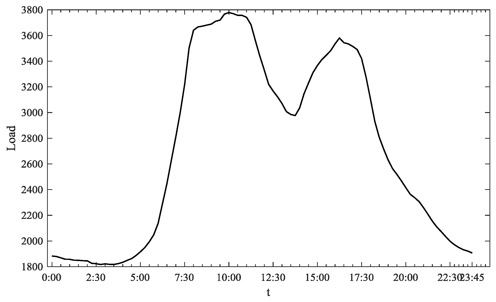
Figure 2 shows the feature of rapid change in the hospital power consumption. Moreover, there are two critical moments of 5:00 and 13:30, after which the hospital’s power load rises sharply in a short time. That is determined by the working hours and the work practices. For alleviating the supply shortage of medical resource, the hospital usually examines and treats inpatients earlier. In that case, the medical equipment and instruments are turned on before the official opening hour of 8:00 a.m. Hence, the power load is relatively stable when the outpatient departments start working. The power load is going to drop after 11:30 and then rise again after 13:30, since the hospital takes a two-hour break at noon when most of the departments and facilities are resting, except for uninterruptible power demand. It is also a fact that Chinese patients prefer to see the doctor or to get examinations and treatments in the morning, which can be reflected from Figure 2 that the power load after reopening in the afternoon is lower than that in the morning.

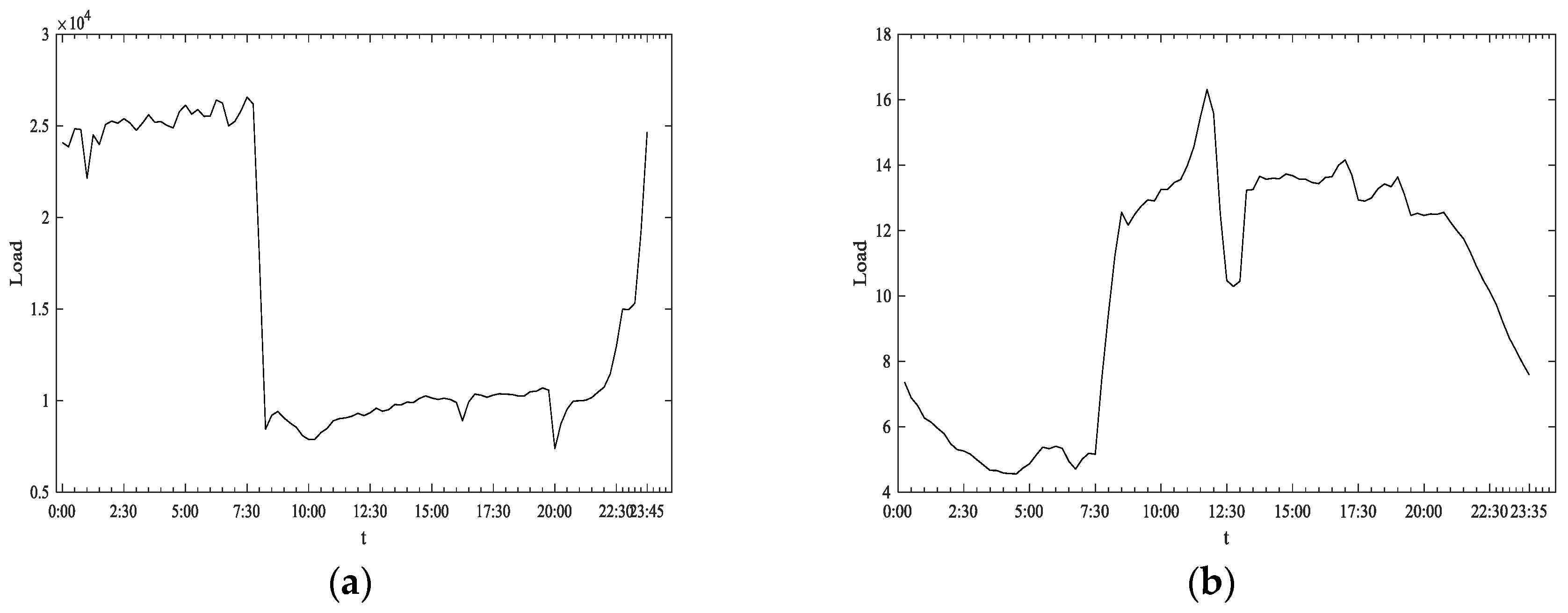
As a public service sector, the hospital behaves quite differently in power consumption when compared with other industry sectors. Taking an individual iron and steel enterprise as an example (see Figure 3a). It consumes the most power among the three sectors, reflecting the massive energy demand of the heavy industry. For easing the power supply pressure and saving costs (the electricity price is much lower during the off-peak time in China), the iron and steel enterprise makes the production activity fit in well with the off-peak time. Also, once the equipment is switched on, the power load is comparatively stable. Contrary to the iron and steel enterprises, the specific textile enterprise (see Figure 3b) that consumes the lowest power resource, is mainly carrying out production activity from 8:00 a.m. to 8:00 p.m. with a very short break during lunch time.

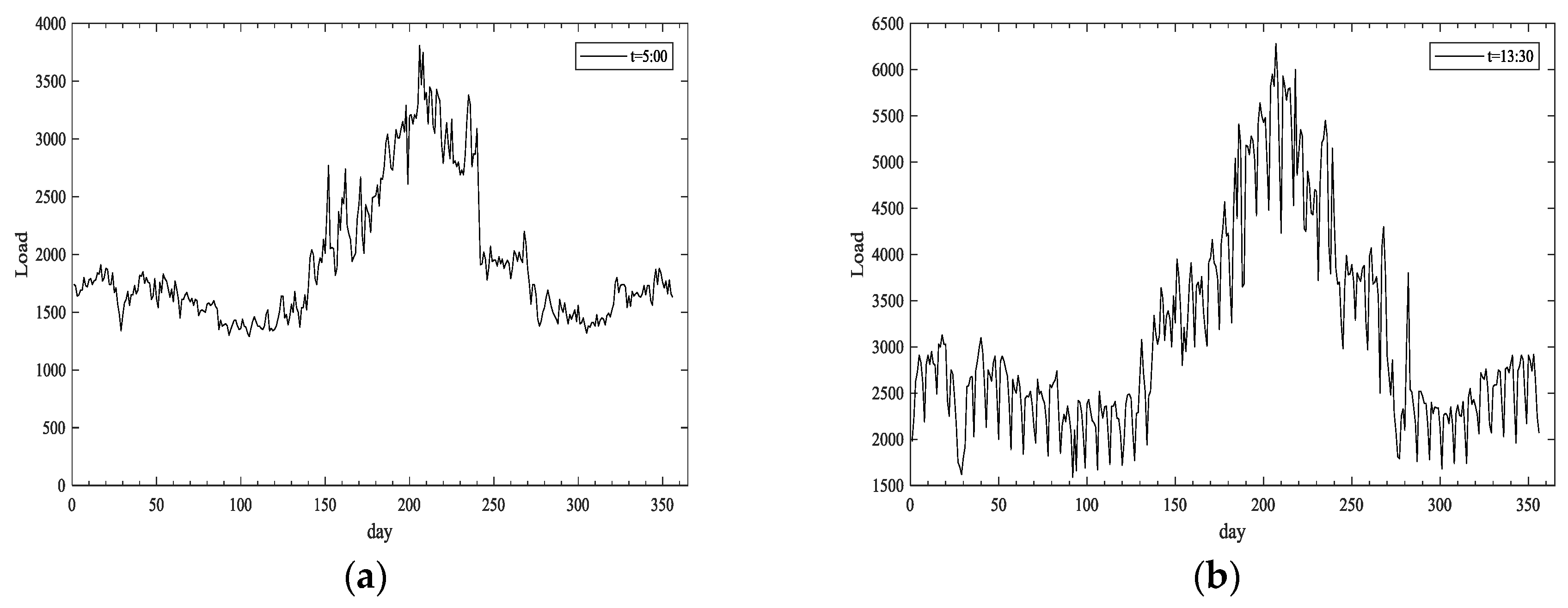
The seasonality of the power consumption of hospital is also a highlight, see Figure 4a,b. From the daily power consumption at moments of 5:00 and 13:30, we can find that as time goes on, the electricity consumption in the hospital continues to rise and reaches the peak in July. After that, with the drop of temperature, the electricity consumption begins to decline, and it never grows again, even in winter. Due to the adoption of gas-powered heating equipment in winter, the electricity demand of the hospital is not as strong as that in summer.

3. Materials and Methods

To pursue the statistical significance of the outcome, extreme events that happen infrequently are usually excluded in the research, intentionally or unintentionally. However, extreme events, with the destructive effect and profound influence, are of great value to study. Therefore, an econophysic method, named recurrence interval analysis, which is aiming at solving extreme events data deficiencies by tracking the scale properties of the data, is introduced in this paper for studying the extreme fluctuations of the hospital power load. Recurrence interval analysis focuses on the time interval between two sequential events. Based on the extreme event that has happened at a specific time, this method can estimate the recurrence probability of next one. This method has been proved efficient in forecasting nature hazards and financial market volatilities [20,21,22]. In practice, by analyzing the characteristics of the recurrence intervals of extreme power fluctuations, our study can help the energy administrator to forecast the hospital power system risk, both in probability and magnitude.

3.1. Methods

The fluctuation of power load is defined as the logarithmic returns of the load in two sequential moments, which is expressed as:

$$v\left(t\right)=\ln l\left(t\right)-\ln l\left(t-\Delta t\right)$$

(1)

where $l\left(t\right)$ is the electricity load (kW) of $t$th time, while ∆t is the frequency of sample data. The logarithmization that was aiming at improving collinearity and heteroscedasticity without destructing the primitive characters of the data is to smooth the data to benefit the further analysis.

As the customary practice in conducting the recurrence interval analysis, time series $v\left(t\right)$ is normalized, as follows:

$$V\left(t\right)=\frac{v\left(t\right)}{{[Ev{\left(t\right)}^2-E^{2}v\left(t\right)]}^{1/2}}$$

(2)

where E indicates the expectation value of variables, hence ${[Ev{\left(t\right)}^2-E^{2}v\left(t\right)]}^{1/2}$ is the standard deviation of $v\left(t\right)$. Given a certain threshold $q$ for the normalized returns, a group number of recurrence intervals $\tau$ will be obtained, which is expressed, as follows:

$$\tau \left(t\right)=\{\min \left(t-t^{\prime }\right):V\left(t\right)>q, t>t^{\prime },q>0\}$$

(3)

Regarding the format of fitting function, the stretched exponential distribution function is overwhelmingly preferred by researchers [11,25,26], which is also our first choice here in this paper. The standard form can be specified as:

$$f\left(x\right)=\alpha \overline{\tau }{\mathrm{e}}^{-{\left(\beta \overline{\tau }x\right)}^{\gamma }}$$

(4)

where α, β, and γ are parameters, and $\overline{\tau }$ is the mean value of recurrence intervals that is determined by threshold q. Hence, the probability distribution of the recurrence interval $\tau$ is $P_q\left(\tau \right)$.

Additionally, to examine the memory effect of recurrence intervals, the short-term correlation and the long-term correlation are both investigated. For verifying the short-term correlation, the conditional probabilities density function $P_q\left(\tau |{\tau }_0\right)$ is introduced to demonstrate the occurrence probability of recurrence interval $\tau$ that follows with last recurrence interval ${\tau }_0$. There are no short-term correlations between recurrence intervals if $P_q\left(\tau |{\tau }_0\right)$ can be proved to be independent from ${\tau }_0$. To verify the long-term correlation, the method of detrended fluctuation analysis (DFA) is utilized to discover whether an abnormal shock will have a long-term effect on the recurrence intervals of the extreme fluctuation [27].

Last but not least, to estimate the recurrence probability of extreme event in a future period $\Delta t$, the hazard probability function is introduced. The theoretical model of the hazard probability function is

$$H_q\left(\Delta t|t\right)=\frac{{\int }_t^{t+\Delta t}{P}_q\left(\tau \right)d\tau }{{\int }_t^{\infty }{P}_q\left(\tau \right)d\tau }$$

(5)

To examine the fitting degree of the hazard probability function, we would calculate the actual probability under different time intervals, which can be expressed as:

$$H_q\left(\Delta t|t\right)=\frac{count\left(t<{\tau }_q\le t+\Delta t\right)}{count\left({\tau }_q>t\right)}$$

(6)

where “$count\left({\tau }_q>t\right)$” denotes the number of recurrence intervals that are longer than $t$ and “$count\left(t<{\tau }_q\le t+\Delta t\right)$” is the number of recurrence intervals belonging to the time interval $(t,t+\Delta t]$ for a given $q$.

3.2. Data

We retrieve the 15-min high-frequency power load data from North Jiangsu hospital, which is measured as kilowatt (kW). The period of the record lasts the whole year of 2017 from 0:00 a.m. of 1 January to 23:45 p.m. of 31 December, which includes 35,040 observations in total. As mentioned above, the return of the power load is defined as the logarithmic difference of the load in two sequential moments, and the descriptive statistics of the returns are shown in

Table 1. The descriptive statistics of the returns v(t).

Mean	Median	Maxi	Mini	Standard Deviation	Skewness	Kurtosis	Nobs
−2.15 × 10−6	−1.97 × 10−3	0.6302	−0.3405	0.0429	0.7935	8.0672	35,039

.

The returns of power load feature the distribution of right-skewed and peak from the report of Table 1. Moreover, it presents the returns the characteristic of the seasonality from Figure 5. For instance, the summer is accompanied by more large returns, while other seasons are accompanied by comparatively smaller ones. Further, Figure 5 provides us with an intuitive impression that large return is more likely to be accompanied by large return, while the small one tends to follow with the small one. This kind of behavior seems like the clustering effect, and a rigorous test will be conducted to support that.

4. The Recurrence Interval Analysis

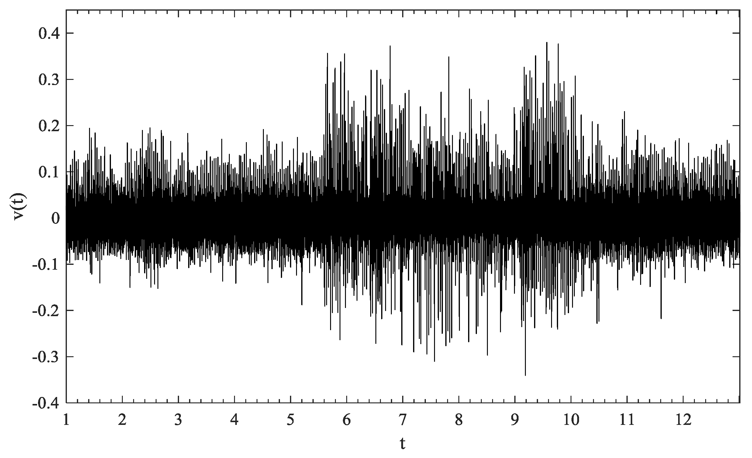
The normalized return of the power load from Equation (2) is named as power load fluctuation. As we have 35,040 pieces of 15-min high-frequency power load data, the time series of power load fluctuations will have 35,039 pieces of data. We give the threshold q as the criterion to determine the magnitude of fluctuation. Any return that is greater or equal to q will be named as an extreme fluctuation. 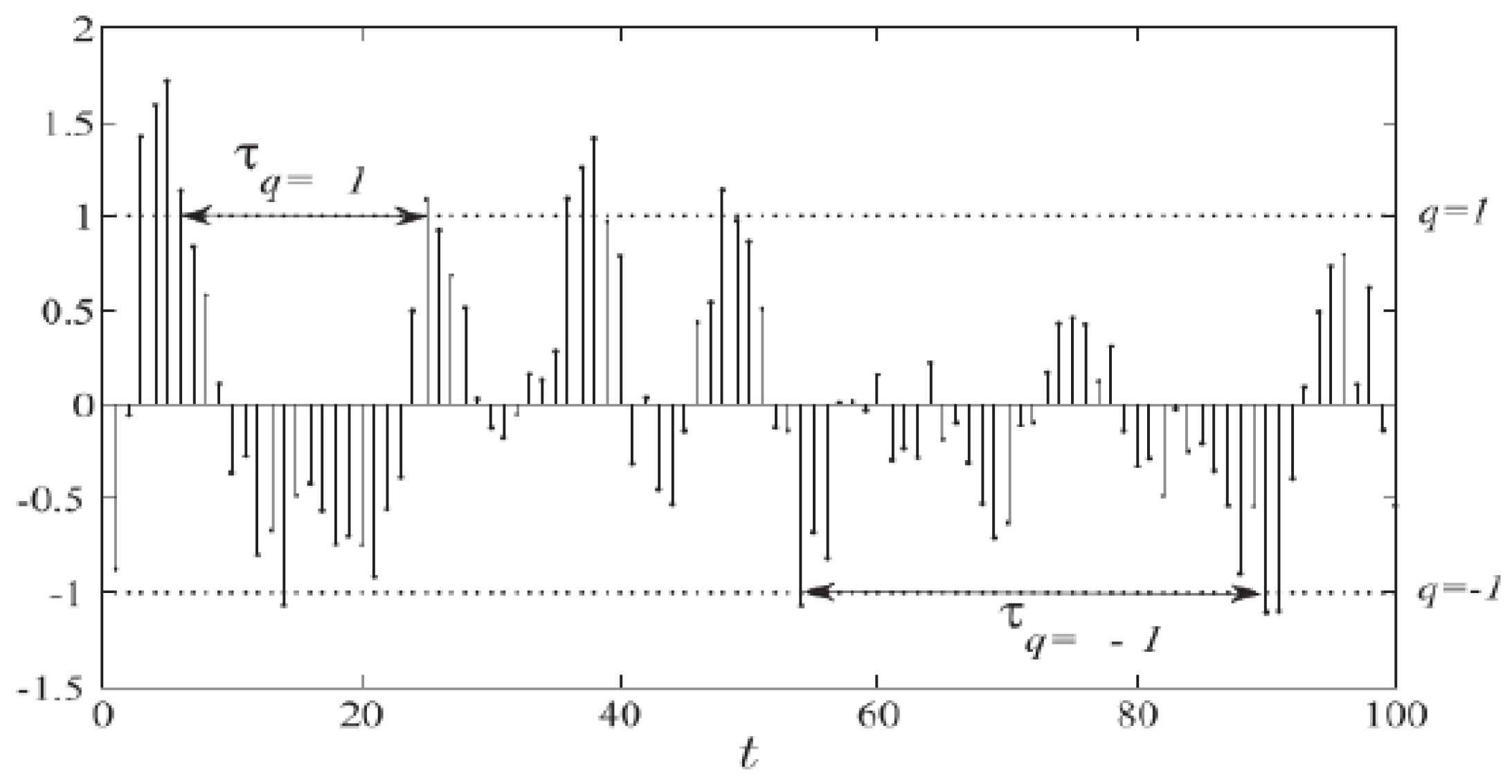In other words, all of the positive fluctuations will be included if we make q = 0. It should be noted that the extreme event in RIA has no particular value any more, but rather a name. We only take positive fluctuations into account, because the positive ones could directly threaten the hospital power system. The time interval between two sequential extreme fluctuations is the recurrence interval, see Figure 6. The criterion of extreme fluctuation is driven up, as the threshold q is increasingly larger.

The conventional practice to determine of threshold is based on the percentile of sample. For example, the threshold of extreme climate is usually set as the 90th or 95th percentile of the sorting sample. Although the threshold q is a man-made selection in this paper, the criterion of extreme fluctuation is also strict. As seen from

Table 2. The statistics of threshold q.

Threshold	Sample Size	Proportion (%)
1.0	3874	11.06%
1.2	2892	8.25%
1.4	2168	6.19%
1.6	1668	4.76%
1.8	1287	3.67%

, the maximum percentage is 11.06%, while the minimum is 3.67%. With the rise of threshold, the sample size is decreasing.

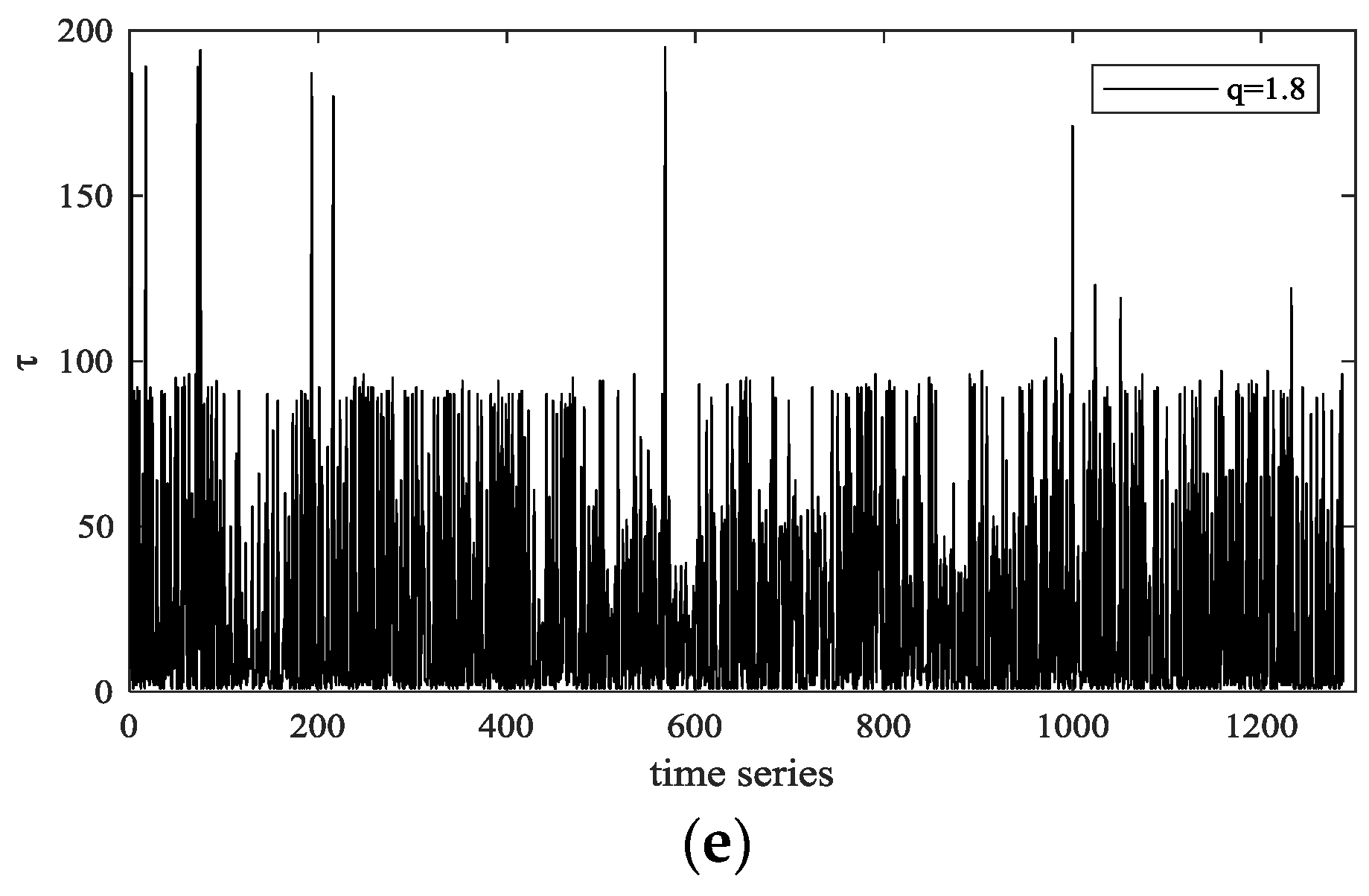
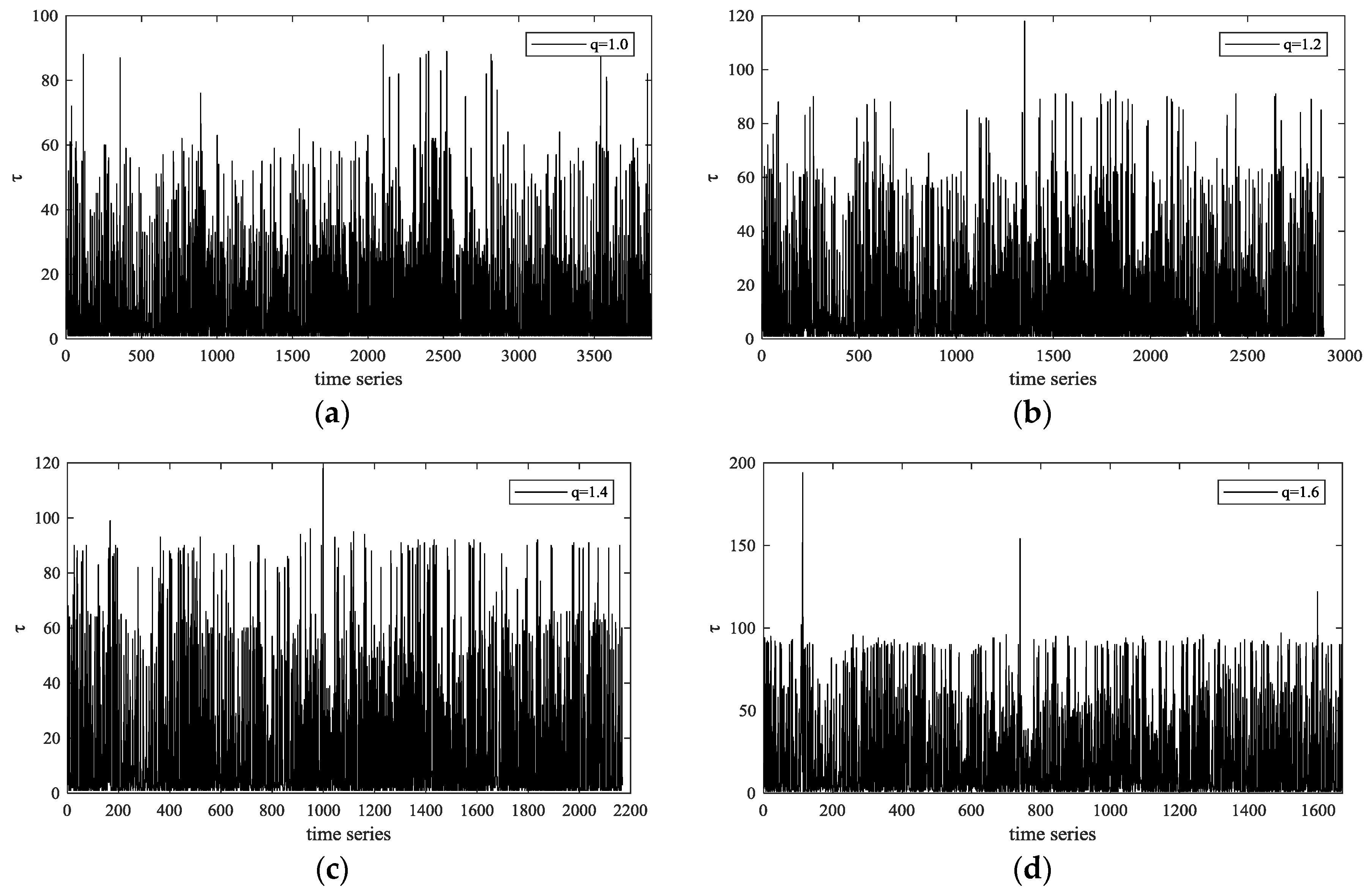
The time series of recurrence interval is transformed from the extreme fluctuations, see Figure 7. The y-axis in all of the subfigures shows the length of recurrence intervals. It seems to have a clustering effect of recurrence interval at first glance of figures, where long interval tends to follow with long interval, while the short one is more likely to follow the short interval.

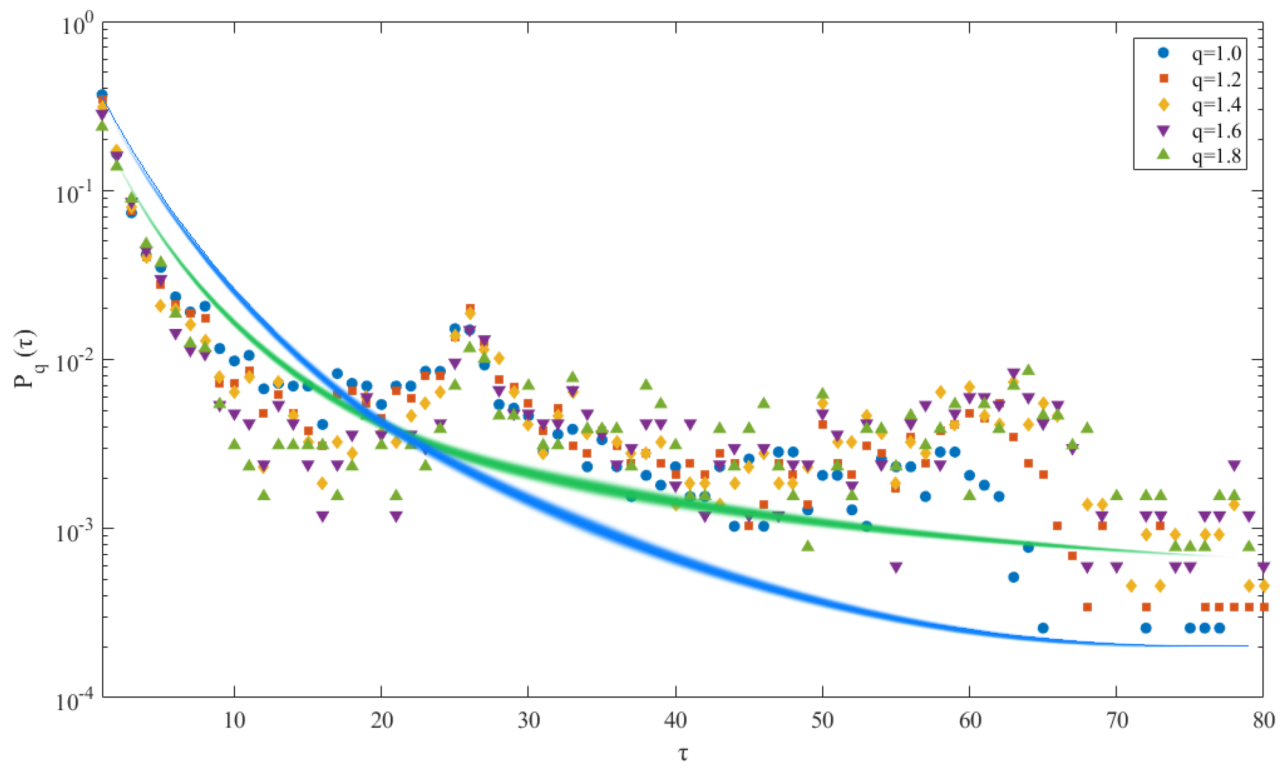
The time series of recurrence intervals with different lengths $\tau$ is obtained, given a specific threshold q. According to Equation (4), the recurrence probability $P_q\left(\tau \right)$ is the function of the time interval $\tau$, as measured in 15 min per unit. As seen from Figure 8, where the y-axis is the logarithm of recurrence probability, the recurrence of the extreme fluctuation come out more often within shorter time intervals. Although only two fitting curves (q = 1 and q = 1.8) are presented for the better visibility, it can be easily imagined that the fitting curve under q = 1 has the peak slope with the largest initial probability and the least probability in the end. The decay of $P_q$ becomes slower for larger q; that is to say, it is more likely to have larger fluctuation since longer peacetime has passed. This outcome is in accordance with the natural rule that the more destructive the natural disasters, the less frequently that they occur. It should be noted that the stretched exponential function might overestimate the recurrence probability of shorter time intervals and underestimate the recurrence of longer time intervals.

In this paper, we use the method of least square to estimate the coefficients of parameters, see

Table 3. The estimates of parameter and the goodness-of-fit of stretched exponential.

Value of q	q = 1.0	q = 1.2	q = 1.4	q = 1.6	q = 1.8
α	3.696	3.918	1.849	1.422	1.097
S.E.	1.6783	1.7171	0.0935	0.0542	0.057
t-value	2.2022	2.2818	19.7754	26.2362	19.2456
Sig.	**	**	***	***	***
β	36.659	54.341	13.05	5.155	3.977
S.E.	3.0248	20.4671	0.122	0.0746	0.097
t-value	12.1195	2.655	106.967	69.1019	41
Sig.	***	***	***	***	***
γ	0.2507	0.2358	0.2483	0.2383	0.2182
S.E.	0.0795	0.0562	0.0899	0.0727	0.0852
t-value	3.1535	4.1957	2.762	3.279	2.561
Sig.	***	***	***	***	**
p-value	0.169	0.2526	0.3049	0.3261	0.421

Note: S.E. is the standard error of the parameter estimate. The t-value could be simply calculated through t = (P.E.)/(S.E.). ***/**/* indicates statistical significance at the 1%/5%/10% level.

. The null hypothesis that the parameter is equal to zero can be rejected with a significant level of at least 5%. Therefore, parameter coefficients estimated by stretched exponential model are reliable. Moreover, a one-sample Kolmogorov-Smirnov test is conducted to check the extent to which the recurrence intervals follow a stretched exponential distribution [28,29,30].

By conducting a one-sample Kolmogorov-Smirnov (KS) test, we assume that the empirical distribution is identical to the best-fitted stretched exponential distribution. The KS statistic is defined, as follows:

$$\mathrm{KS}=\max \left(\left|F_q-F_{SE}\right|\right), q\in \left\{1.0, 1.2, 1.4, 1.6, 1.8\right\}$$

(7)

where $F_q$ is the cumulative distribution under certain threshold, while $F_{SE}$ is the cumulative distribution from integrating the fitted stretched exponential.

Then, we adopt the bootstrapping method to do the calculation. 1000 synthetic samples from the best-fitted distribution are first generated, and then the cumulative distribution $F_{sim}$ of simulated sample and its cumulative distribution function (CDF) from integrating the fitted stretched exponential are reconstructed. Therefore, the KS statistic between the fitted CDF and the simulated CDF can be written as:

$${\mathrm{KS}}_{sim}=\max \left(\left|F_{sim}-F_{sim, SE}\right|\right)$$

(8)

The probability that ${\mathrm{KS}}_{sim}$ is greater than $\mathrm{KS}$ is reported in the last raw of Table 3. As can be seen from Table 3, all of the P-values are greater than 0.1, which means that the null hypothesis that the empirical probability distribution function is well fitted by a stretched exponential cannot be rejected, even at the significance level of 10%. In other words, the stretched exponential has a good fit to the empirical probability distribution functions. Moreover, the goodness-of-fit is improved with the rise of threshold q.

4.1. The Analysis of Abnormal Values

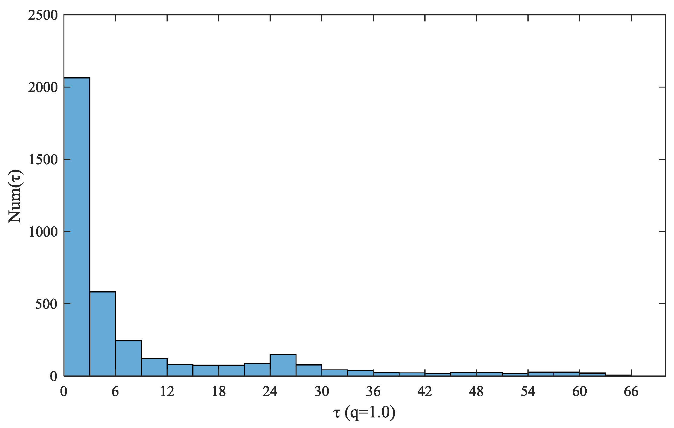
As seen from Figure 8, there is a jump that exists markedly in the downward trend. To make it clear, we take q = 1 as the example to build a bar graph of recurrence intervals distribution that is shown in Figure 9.

As seen clearly from Figure 9, it shows the trend that the longer time that the interval runs, the less extreme fluctuations recur. However, there is a special case that exists in the time interval of around six to seven hours (The unit of time interval is 15 min, which means 24–27 units’ interval is approximately equal to six to seven hours), in which the extreme fluctuation recurs more times than that in neighbor time intervals. The hospital schedule may be the main reason for that abnormality. As mentioned above, the primary power consumption of North Jiangsu hospital ends at 22:00 and it starts again at 5:00 in next morning, which means that there are about seven hours when the power load stays at a stable low level. The power load experiences a sudden rise after 5:00, and that leads to large volatilities. Hence, it is a golden opportunity for energy manager to make use of the vacant seven hours to smooth the power consumption in the hospital.

4.2. Scaling Behavior

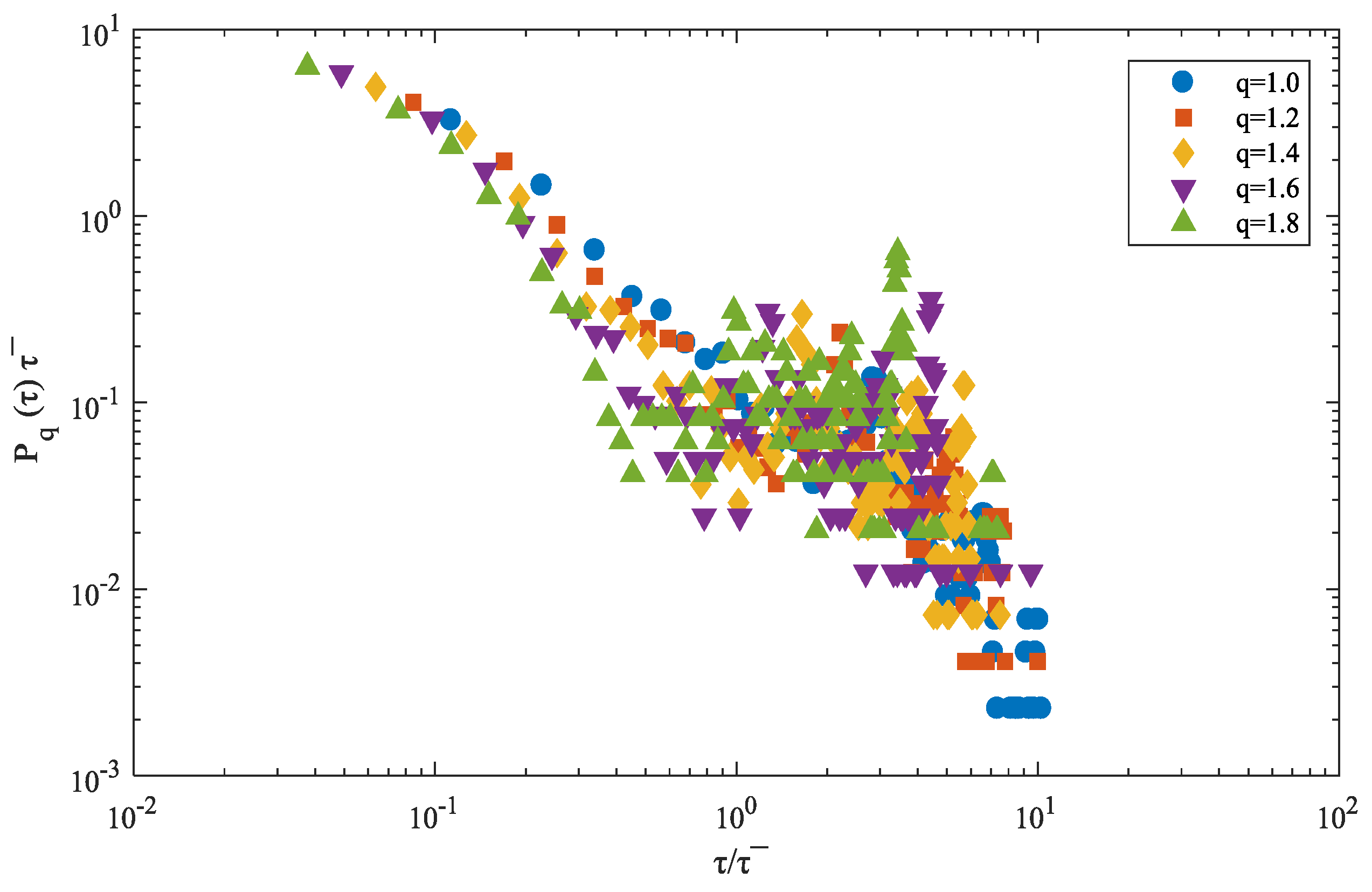
When considering the similar shape of curves in Figure 8, we will conduct a Yamasaki method [31] to detect whether scaling behaviors exist in different probability distributions of recurrence intervals. We start with introducing $\tau /\overline{\tau }$ as the scaled recurrence interval, in which $\overline{\tau }$ is the average recurrence interval. The scaling $f_q\left(\tau /\overline{\tau }\right)=P_q\left(\tau \right)\overline{\tau }$ is a function of $q$ as $\tau$, and $\overline{\tau }$ vary with threshold $q$ in the same direction. If $f_q\left(\tau /\overline{\tau }\right)$ is independent to $q$, all of the functions will converge to a unique function $f\left(x\right)$, which can be derived as $f_q\left(x\right)=f\left(x\right)$ [32]. Namely, recurrence intervals will be scaled with the scaled probability distribution $f_q\left(\tau /\overline{\tau }\right)$ converges to $f\left(\tau /\overline{\tau }\right)$. 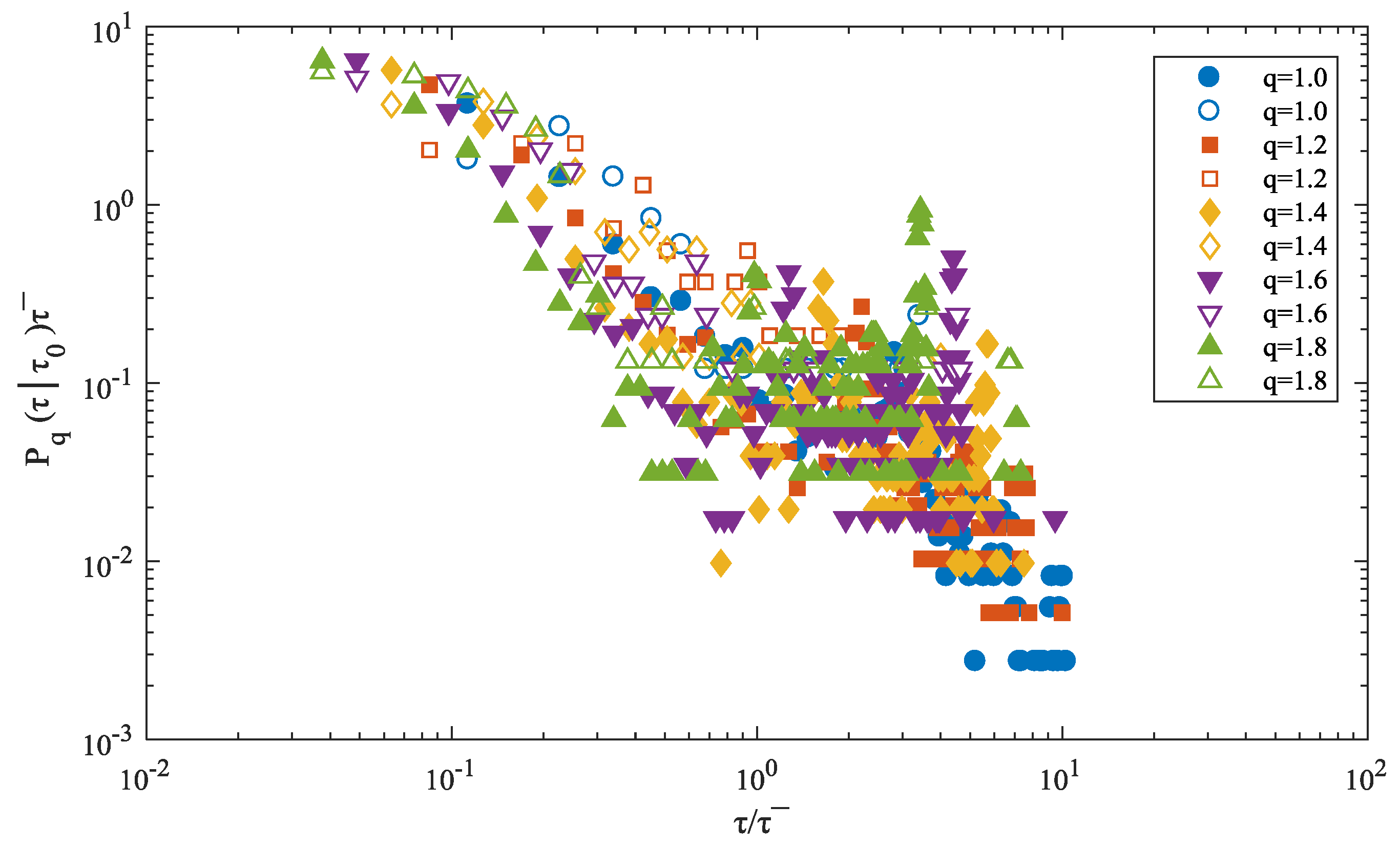To verify that the scatter diagram of $f_q\left(\tau /\overline{\tau }\right)$, which is designed as the function of $\tau /\overline{\tau }$, is shown in Figure 10.

It is clear that the scaled probability distributions with different thresholds do not feature the convergence, which is a refusal to the speculation on the scaling behavior. In practice, it tells us that the large fluctuations of power load cannot be inferred from the small fluctuations.

The Yamasaki method is more of a graphical test on scaling behavior. There are some well-established statistical methods that are based on properties of regularly-varying functions and power-law behavior in the upper tail to test the scaling of sample distribution [33]. Based on the feature of this study, a two-sample KS test is adopted to check the scaling behavior statistically.

The KS test principles allow for us to test whether two samples have the same distribution, which means that there is scaling if $F_{qi}=F_{qj}$ is proved significantly. Denoting $F_{qj}$ as the cumulative probability function of $f_{qj}$, then the KS statistic could be calculated by comparing two cumulative distribution functions.

$$\mathrm{KS}=\max \left(\left|F_{qi}-F_{qj}\right|\right), q_i\ne q_j$$

(9)

The null hypothesis of $F_{qi}=F_{qj}$ will be rejected if the KS statistic is larger than the critical value (CV). The critical value is expressed as:

$$\mathrm{CV}=c\sqrt{\frac{\left(m+n\right)}{mn}}$$

(10)

where m and n are the numbers of recurrence interval samples for $q_i$ and $q_j$, respectively. $c$ is a threshold here with certain value ($c=1.63$ at the significance level of 1%, 1.36 at 5% and 1.22 at 10%). It is clear from

Table 4. Two sample Kolmogorov-Smirnov test of scaling behavior with critical value (CV) at significance level of 5%.

qi	qj	KS	CV
1.0	1.2	0.648	0.033
1.0	1.4	0.718	0.037
1.0	1.6	0.732	0.040
1.0	1.8	0.741	0.044
1.2	1.4	0.653	0.039
1.2	1.6	0.631	0.042
1.2	1.8	0.641	0.046
1.4	1.6	0.544	0.044
1.4	1.8	0.536	0.048
1.6	1.8	0.454	0.051

that KS is always much greater than CV in any case, which means that there is no scaling behavior that exists in the distribution of recurrence intervals for different thresholds.

4.3. Memory Effect

The relationship between two observations of time series is usually measured by their autocorrelation function. In stationary time series, the degree of correlation between the two observations at the different time depends on the lag order of $n$, and as $n$ increases, the degree of correlation decays gradually to zero. The memory effect of the time series is characterized by the decay rate of correlation. If the autocorrelation function quickly converges to zero with the increase of lag order, then it is named as short-term memory effect, and vice versa, is long-term memory effect.

In the scenario that the previous time interval is ${\tau }_0$, the conditional probability density function $P_q\left(\tau |{\tau }_0\right)$ measures the recurrence probability of extreme fluctuation after time interval $\tau$. If $P_q\left(\tau |{\tau }_0\right)$ is found to be independent of ${\tau }_0$, then it means that there is no short-term correlation [34].

We could have selected any two of sequential recurrence intervals to make a comparison, but we enlarge the scope of comparison for the rigorous purpose. By arranging the recurrence intervals that are determined by a specific threshold $q$ in ascending order, and then dividing them equally into four disjoint subsets with the same size as $S=S_1\bigcup S_2\bigcup S_3\bigcup S_4$ where $S_i\bigcap S_j=\varphi$, $i\ne j$, the smallest quarter of the sorting intervals are in subset $S_{1 }$, while $S_4$ contains the largest quarter of S. If the Equation (11) is true, then there is no short-term correlation. To verify this, we draw the scatter diagram of $P_q\left(\tau |{\tau }_0\right)\overline{\tau }$ as a function of $\tau /\overline{\tau }$ in Figure 11.

$$P_q\left(\tau |S_i\right)=P_q\left(\tau |S_j\right),i\ne j$$

(11)

As seen from the figure, where the filled dots are from $S_4$ and hollow dots are from $S_1$, distributions from all the subsets do not feature the superposition properly, which means $P_q\left(\tau |S_i\right)\ne P_q\left(\tau |S_j\right)$. Hence, there is the short-term correlation. Additionally, we also find that $P_q\left(\tau |{\tau }_0\in S_1\right)$ is larger than $P_q\left(\tau |{\tau }_0\in S_4\right)$ when $\tau /\overline{\tau }$ is small, but $P_q\left(\tau |{\tau }_0\in S_4\right)$ will be greater than $P_q\left(\tau |{\tau }_0\in S_1\right)$ when $\tau /\overline{\tau }$ is large. This indicates a fact that a short recurrence interval is more likely to follow a short one, while a long time interval tends to follow a long recurrence interval. As a conclusion, the existence of short-term memory effect implies that there is a great possibility that an extreme fluctuation of the power load will recur very closely if the last recurrence interval is short.

To examine the robustness of short-term dependence of recurrence interval, a permutation test is adopted [35]. The permutation test focuses on comparing the observed value of statistic with the permutation distribution of that statistic. If there is some dependence structure in data, then the observed value should be extreme with respect to this reference distribution.

The outcome is achieved by generating 1000 permutations of the time series. As seen clearly from

Table 5. The permutation test for independence of recurrence intervals.

The Value of q	q = 1.0	q = 1.2	q = 1.4	q = 1.6	q = 1.8
c	599	720	928	452	443
p-Value	0.599	0.72	0.928	0.452	0.443
S.E. of p	0.0155	0.0142	0.0082	0.0157	0.0157
Reject H0	N	N	N	N	N

, all of the p-Values are reliable concerning the standard error of each. The null hypothesis of independence of data cannot be rejected at any significant level. Therefore, the short-term dependence of recurrence intervals statistically exists.

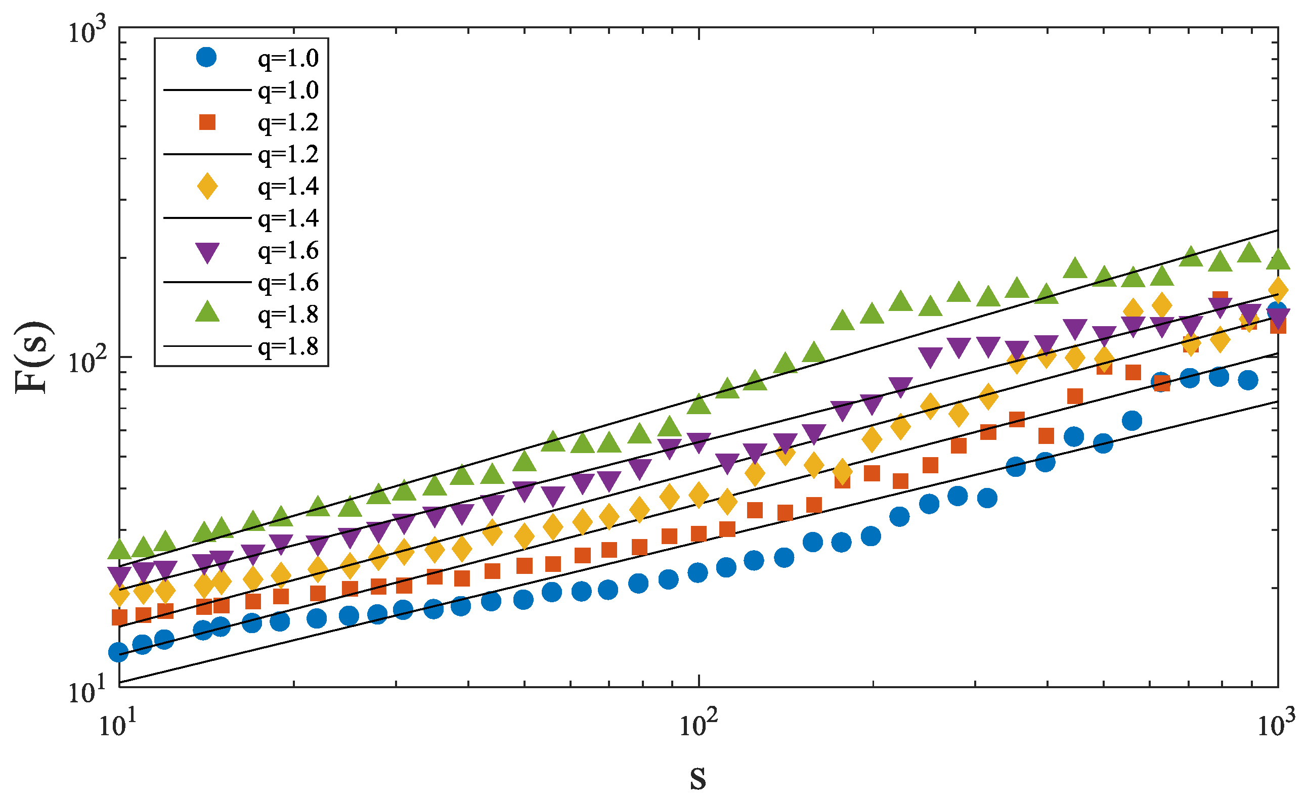
Speaking from financial research experience, the fluctuations in the time series usually have the long-term memory effect in the long run [36]. However, whether this rule regularly applies to recurrence interval series of extreme volatilities is still unknown. To study the long-term memory effect of the recurrence intervals, we utilize the method of detrended fluctuation analysis (DFA) in order to investigate the long-term correlations among recurrence intervals.

The DFA method is first invented in 1994 and has been employed as an authoritative way to detect the long-term correlations in a time series since then [37,38,39]. The necessary steps that are involved in conducting a detrended fluctuation analysis are as follows:

(a)

Calculating accumulated deviations of original data to build a new time series:

$$Y=\left\{y\left(i\right)={\displaystyle \sum }_{N=1}^i\left({\tau }_i-\overline{\tau }\right), N=1, 2,\dots , n\right\}$$

(12)

(b)

Dividing new series $Y$ into $m$ subsets with the same s, where $m=\frac{n}{s}$, and then using the Ordinary Least Squares method (OLS) to do the first order linear fitting of the data in each subset.

(c)

Calculating the mean squared errors (MSE) whose trends have been filtered:

$${\epsilon }_i\left(s\right)=y_i-{\tilde{y}}_i\left(s\right)$$

(13)

(d)

Computing the root-mean-square deviation of each subset to get the volatility function of DFA, which is expressed as:

$${\left[F\left(s\right)\right]}^2=\frac{1}{n}{\displaystyle \sum }_{i=1}^m{\left[{\epsilon }_i\left(s\right)\right]}^2$$

(14)

(e)

Calculating the $F\left(s\right)$ for a range of different $s$, a log-log figure of $F\left(s\right)$ against $s$ is constructed in accord to the form $F\left(s\right)~s^H$. The H here is the Hurst exponent, which is used to determine whether the time series have a long-term correlation, see

Table 6. The explanations of Hurst exponent.

The Range of Values	Meaning
0.5 < H < 1	Indicating the existence of long-term correlation in the time series, and with closer to 1 the stronger correlation will be.
H = 0.5	Indicating an independent random process, which means the current volatility will not affect the future.
0 < H < 0.5	Indicating the anti-continuity feature that the volatility has a negative influence on the future volatility.

.

Combining Figure 12 with

Table 7. The Hurst exponents under different thresholds.

Threshold q	Hurst Index
q = 1.0	0.42599
q = 1.2	0.45650
q = 1.4	0.49655
q = 1.6	0.44758
q = 1.8	0.50938

, it is clear that most Hurst exponents are smaller than 0.5, suggesting that the long-term correlations do not exist in the time series of recurrence interval, or at least, the inference on the long-term memory effect is the lack of evidence. Namely, it is not a one-time practice for power load volatilities forecasting, and the energy plan, aiming at improving power efficiency, has to be fixed and updated continuously by tracking the power load change in the short term, which puts a heavy responsibility on the energy manager in the hospital.

4.4. Risk Estimation

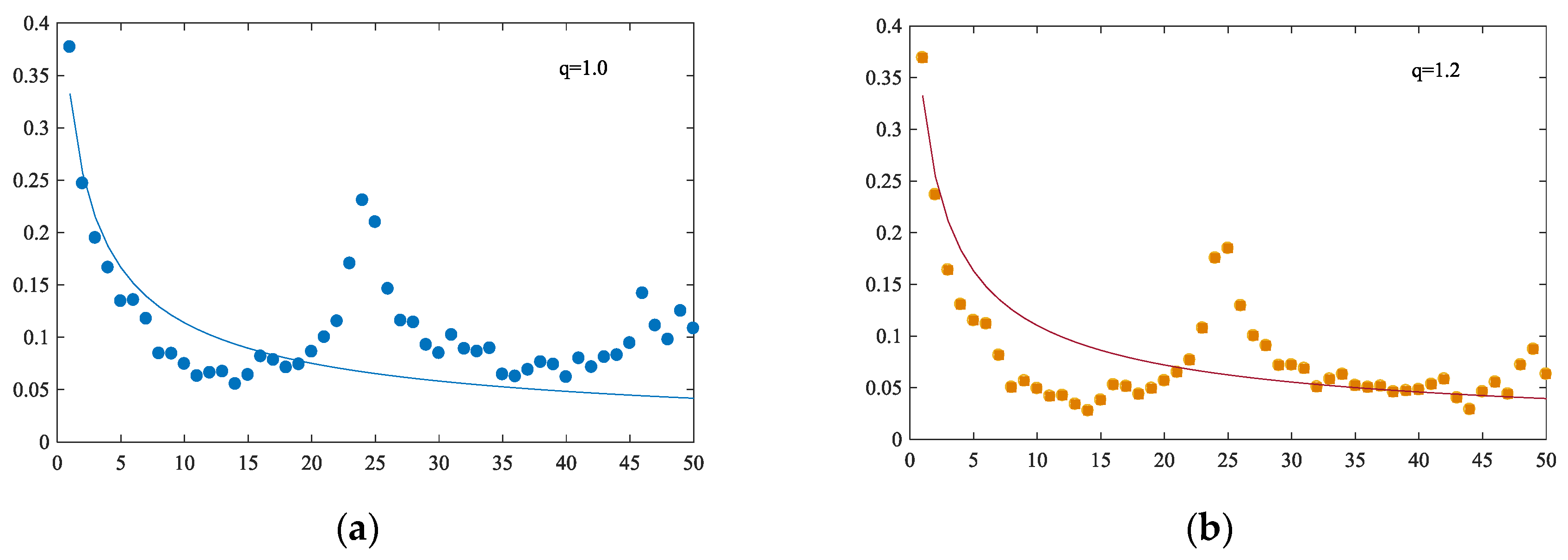
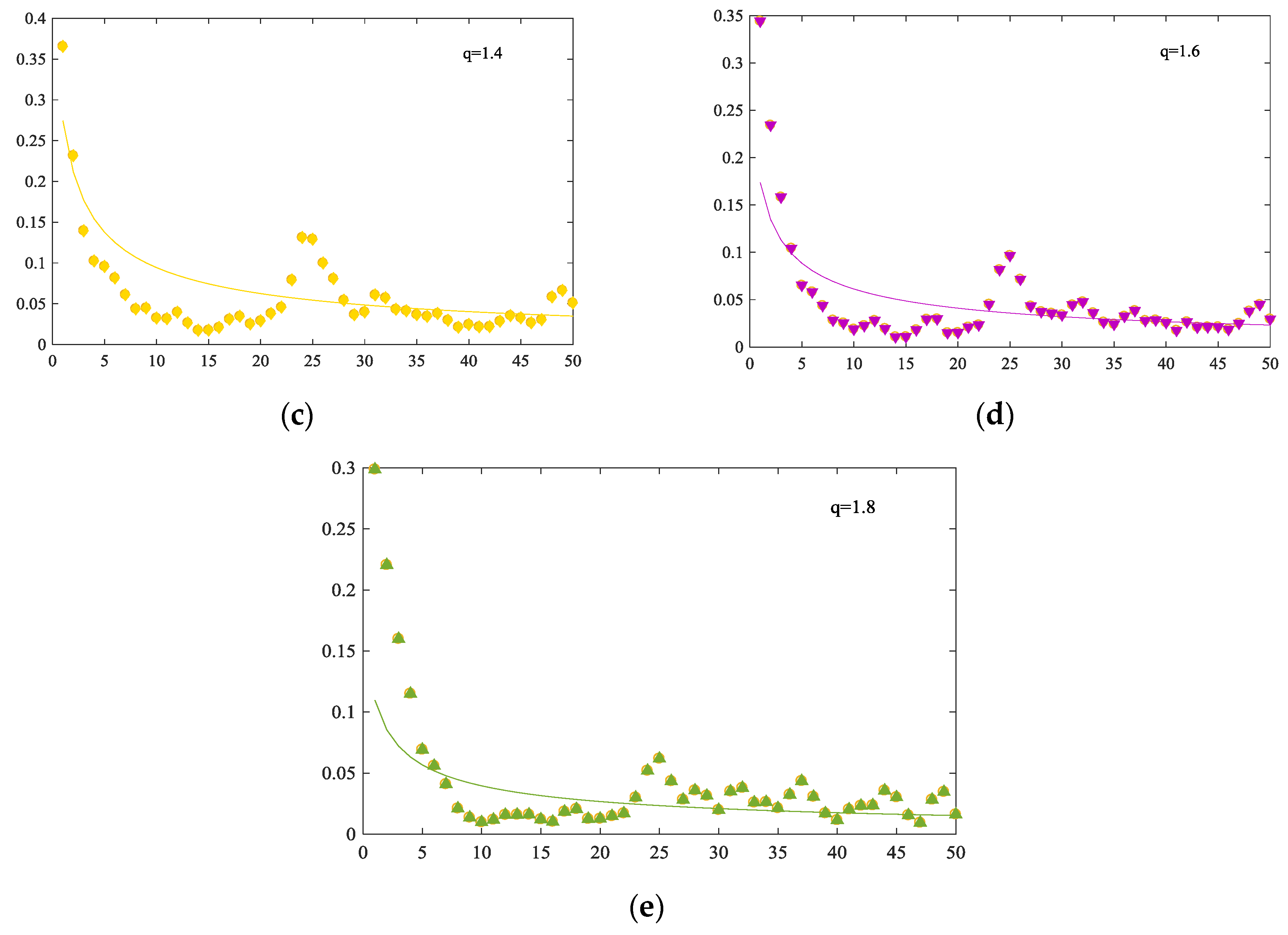
For the energy manager of the hospital, besides the extreme power fluctuation that has already occurred, the recurrence probability of next extreme volatility is more of a matter to concern. To estimate the recurrence risk, we introduce the hazard probability function, which has been covered in the last section [40]. Figure 13 shows the scatter plots as well as the fitting curves of the hazard probability function. The horizontal axis indicates the length of time intervals, while the vertical axis is the hazard probability of $H_q\left(\Delta t=15|t\right)$.

As seen from Figure 13, the risk probability of extreme volatilities recurrence decreases along with the increase of time interval, and, by that, the cluster behavior of recurrence intervals has been proved once again. Moreover, the discrepancy between real and theoretical values is increasingly narrowing with the increase of the recurrence interval. However, Figure 13 also tells us that the long-term memory effect may not exist in the time series of recurrence intervals as a sudden rise appearing in the middle of the horizontal axis. As a result, the hazard probability function cannot fit the scatter plots in the mid-term ($\Delta t\in \left(20, 30\right)$).

In practice, the hazard probability function can be used to estimate the future risk of extreme volatility of hospital power consumption. However, the energy administrator has to be very careful that the mid-term estimation error may increase.

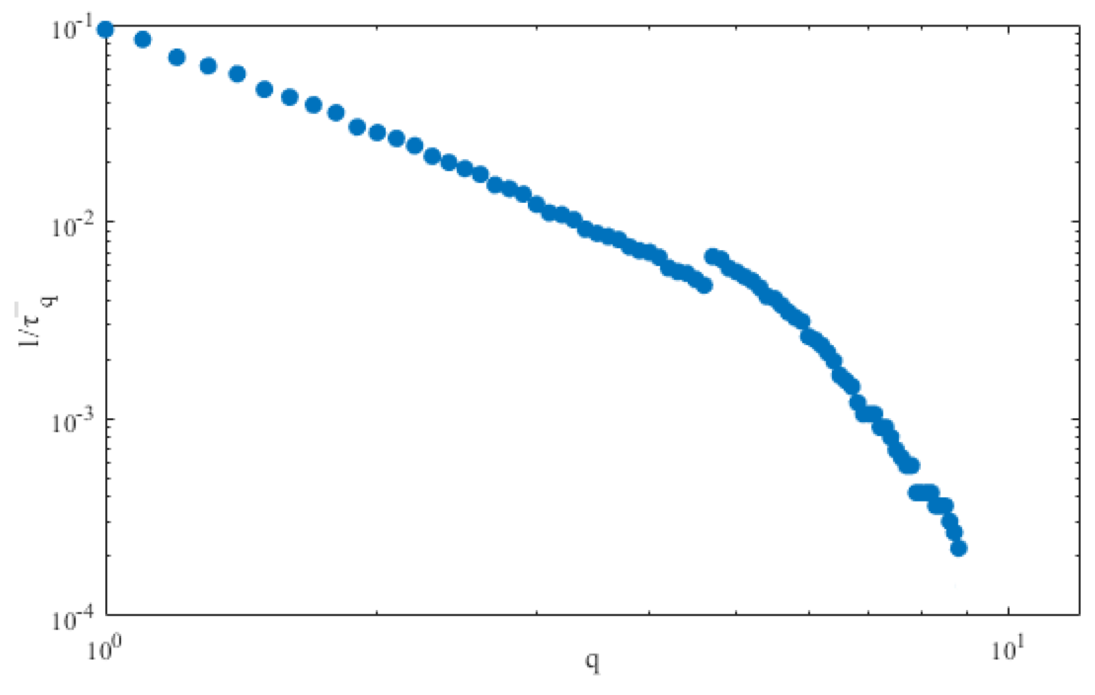
To motivate the risk estimation analysis, we adopt the method of Value at Risk (VaR) [41]. We use the loss probability density function to estimate the VaR, which is written as ${\int }_q^{+\infty }P\left(V\right)dV=P^{*}$. $P^{*}$ defines the probability to lose the amount of $q$, while $P\left(V\right)$ is the probability distribution function (PDF) of time series of $V\left(t\right)$. Based on the integral principle, it is easy to infer that the loss probability is also equal to the ratio of samples whose return is no smaller than $q$ to total sample size of $V\left(t\right)$. Hence, the $P\left(V\right)$ can also be written as:

$$P^{*}={\int }_q^{+\infty }P\left(R\right)dR=\frac{samples \ge q}{total sample size of V\left(t\right)}$$

(15)

As seen from Figure 6, the total length of recurrence intervals is approximately equal to the total sample size of the times series $V\left(t\right)$. The mean recurrence interval is ${\overline{\tau }}_q=\frac{1}{N_q}{\sum }_{i=1}^{{\tau }_q}{\tau }_{q,i}$, hence the number of returns that is no smaller than $q$ is $N_q+1$. Then, the $P\left(V\right)$ can be rewritten as

$$P^{*}={\int }_q^{+\infty }P\left(R\right)dR=\frac{samples \ge q}{total sample size of V\left(t\right)}=\frac{1}{{\overline{\tau }}_q}$$

(16)

By doing that, the VaR of recurrence intervals can be presented as a function of $\frac{1}{{\overline{\tau }}_q}$ and $q$, which is also shown in Figure 14. The reciprocal of mean recurrence interval decreases with the rising of $q$, suggesting a longer time interval with a larger fluctuation. The VaR method is quite useful in practice. The hospital energy administrator can roughly estimate the risk probability (loss = q) of the next occurrence. For example, if a risk probability of 10% is acceptable by the hospital, then the energy administrator can easily find the criterion of extreme fluctuation by making $1/{\overline{\tau }}_q =10\text{\%}$.

More importantly, Figure 14 also indicates the difficulty in forecasting hospital power load fluctuation. As there is an inflection point that exists at $q\approx 7$, the scatters cannot be fitted by only one empirical distribution. The declining trend is speeding up after the inflection point, which requires more attention.

5. Conclusions

How to balance the electricity efficiency and electrical safety is a tough job for the hospital energy administrator. This paper may provide a new perspective for this dilemma. As a sudden surge of power consumption could endanger the medical instruments and hospital power system, it is of theoretical value to detect the feature of power load fluctuations. Also, it is of practical value to forecast the risk of extreme fluctuations to avoid potential hazard (e.g., fire caused by short circuit).

Based on 15-min high-frequency power load date, this paper utilizes the method of recurrence interval analysis to investigate the instantaneous features of power load fluctuation in a Chinese hospital. As a result, the stretched exponential function statistically fits with the probability distributions of the recurrence interval. Secondly, the inexistence of scaling behavior makes it impossible to infer large (small) fluctuation from small (large) fluctuation. Additionally, the clustering effect is confirmed from the short-term dependence of recurrence intervals, as only the short-term memory effect has been proved. Last but not the least, the VaR method is proposed to accurately estimate the risk probability at a certain loss.

On the basis of the statistical and empirical analyses, the following suggestions are summarized for the hospital energy administration:

By empirical analyses above, the recommendations for improving the power efficiency of the hospital are summarized: Firstly, when considering the seasonality of power consumption in hospital, it will be a good choice for the energy administrator to take seasonal differential practice. For example, more efforts should be taken to store power and to make ice during the off-peak time in the summer to improve electricity efficiency and to save on the bill. Secondly, as the power consumption often fluctuates drastically, the energy administrator should conduct frequent and prospective inspections on power devices and equipment in a timely manner to avoid hazard. Thirdly, since only the short-term memory effect exists, it is not a one-time practice to forecast the fluctuation. To ensure the forecast accuracy, the energy administrator has to update and process power load data timely. Fourthly, as the extreme fluctuation is more likely to reoccur in a short time while the more serious fluctuation is more likely to appear in a long time, the energy administrator need to avoid fluke mind and to keep concentration. Last but not least, the risk probability needs to be adjusted according to the threshold of loss, as there is an inflection point that exists at $q\approx 7$.