Abstract
Convergence performance and optimization efficiency are two critical issues in the application of commonly used evolution algorithms in multi-objective design of wind turbines. A gradient-based multi-objective evolution algorithm is proposed for wind turbine blade design, based on uniform decomposition and positive-gradient differential evolution. In the uniform decomposition, uniformly distributed reference vectors are established in the objective space to maintain population diversity so that the population aggregations, which are commonly observed for wind turbine blade design using gradient-free algorithms, are minimized. The positive-gradient differential evolution is introduced for population evolution to increase optimization efficiency by guiding the evolutionary process and significantly reducing searching ranges of each individual. Two-, three- and four-objective optimizations of 1.5 MW wind turbine blades reveal that the proposed algorithm can deliver uniformly distributed optimal solutions in an efficient way, and has advantages over gradient-free algorithms in terms of convergence performance and optimization efficiency. These advantages increase with the optimization dimension, and the proposed algorithm is more suitable for optimizations of small size populations, thus remarkably enhancing the design efficiency.
1. Introduction
As a key wind turbine component, the blade is a determining factor for energy harvesting efficiency, while producing and withstanding loads. This makes it imperative that the blade should be designed based on its compatibility with the turbine, and thus wind turbine blade design is a process that includes multiple systems-level and component-level optimization objectives that are sometimes in conflict with one another [1]. Various design variables and constraints are involved in describing the blade aerodynamic shape and structural layout, as well as meeting the geometric, load, stress and strain, vibration, and fatigue requirements of the system. In a typical design example [2], up to 32 design variables and 102 constraints are adopted in optimizing a wind turbine, resulting in an extremely challenging design process.
Recently, multi-objective design has been intensively studied and widely applied in wind turbine design [3,4]. Multi-objective optimizations stand in contrast to singular optimal solution. Multi-objective optimizations constitute a group of trade-off solutions (known as Pareto optimal solutions) as a result of compromise of several optimization objectives. A Pareto Front (PF) is achieved through this compromise. Currently, multi-objective optimization of wind turbines is all achieved by evolution algorithms, including the hierarchical genetic algorithm [5], Pareto archived evolution strategy [6], strength Pareto evolutionary algorithm 2 [7,8], multi-objective genetic algorithm [9], non-dominated sorting genetic algorithm-II (NSGA-II) [10,11,12,13] and particle swarm optimization (PSO) [14,15]. These algorithms are categorized as gradient-free algorithms (GFAs) [16]. Advantages of GFAs include excellent tolerance for random errors that occur in the search process and applicability in optimization using several design variables, objectives, and constraints. However, GFAs are limited by their low efficiency, poor convergence performance, and the possibility that they may not achieve accurate PFs [17]. These limitations are caused by three factors.
The first factor is that the optimization efficiency of GFAs degrades drastically as design variables increase, as detailed illustrated in the reference [16], where the PSO algorithm is used as a typical GFA and the Rosenbrock function is used as the standard function. The similar trend has also been observed in the design of the aerodynamic shape of wind turbine blade that has been reported elsewhere [18]. As observed, the number of function evaluations of GFAs required for optimization convergence increase quadratically with the number of design variables. Over 10,000 evolution generations are required to converge in the optimizations where more than ten design variables are involved, which are commonly observed in wind turbine design [11]; this results in unacceptable computational burdens. Additionally, it can be concluded from the research that gradient-based algorithms can significantly increase optimization efficiency. Despite efforts to apply gradient-based algorithms to the single-objective optimization of a wind turbine [16,19,20], few gradient-based algorithms have been applied in multi-objective optimization of a wind turbine [11].
The second factor that limits GFAs is the issue of dimensionality [21]. In GFAs, the Pareto dominance principle is the criterion for the comparison of individuals and the major driving force for population evolution. The Pareto dominance principle looks for the solution that is better in terms of at least one objective, and is not worse than another solution on any objective. The probability that an individual can evolve into an improved performance is 1/2m (m is the number of objectives) [17]. For instance, the probability in a quadruple-objective optimization is 1/16. Clearly, the probability decreases as the optimization dimension increases, making the algorithm pre-disposed to failure. To date, most wind turbine designs have adopted double-objective optimization strategies; few optimizations adopt triple-objective strategies, which involve considerable simplifications. GFAs are not used in designs with high dimension optimization strategies due to the extremely challenging optimization process.
The third factor limiting GFAs is their ineffective diversity maintaining mechanism, which can result in unacceptable population distributions that in turn affects the convergence performance of the algorithm. GFA diversity is maintained by clustering operators [5,6,7] and crowding distance [9,10,11,12,13], as well as their variants [14,22], and assigning a virtual value to each individual in order to provide clues for the approximated value of the density of the adjacent solutions. As the distances from a specific solution to adjacent solutions increase, this value increases, and therefore results in an increasing probability that the specific solution is selected. In cases involving these two mechanisms, population distributions are dynamically regulated for all generations, which causes performance fluctuations and efficacy degradation. Population aggregation induced by ineffective diversity maintenance can be observed, and an accurate PF cannot be achieved [17,23].
Convergence performance and optimization efficiency, the two crucial factors for optimization, are significantly challenging in cases where conventional GFAs are applied in multi-objective design of wind turbine blades. To solve this problem, a gradient-based differential evolution algorithm is proposed based on uniform decomposition and positive-gradient evolution, named as the MODE/D&P algorithm, in this article. Both the aerodynamic models and the structural models are established. These models are embedded into the MODE/D&P algorithm, where the blade aerodynamic performance and structural dynamic response are also evaluated in the design process. Based on this design framework, two-, three- and four-objective optimizations of 1.5 MW wind turbine blades are carried out, followed by detailed performance evaluation of the proposed algorithm in multi-objective design of wind turbine blades.
2. Modelling of Wind Turbine Blade
2.1. Block Diagram Structure and Procedures for Blade Optimization
The block diagram structure for the optimization of wind turbine blade is shown in Figure 1, where there exist three main modules: blade modelling, optimization, and simulation.
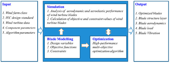
Figure 1.
Block diagram structure of a wind turbine blade optimization.
The design variables, objectives and constraints for optimization are defined in the part of blade modelling. In the optimization part, a high-performance optimization algorithm is developed to deal with the complex optimization based on decomposition and differential evolution. Detailed descriptions of the proposed algorithm are given in Section 3.
In the simulation part, aeroelastic calculations of wind turbines are performed for determinations of the objective and constraint values of each solution. It is important to point out that the determination of the extreme loads acting on the wind turbine, prerequisite for structural design, is a complicated and complex task involved in nonlinear simulations of aero-elastic-hydro-servo interactions in thousands of design load cases. In this study, the extreme loads are evaluated using the FAST [24], which is widely-used software packages for wind turbine dynamic performance analysis, and have been tested and validated by several kinds of wind turbines [25,26,27,28]. The wind class and design load conditions are set in terms of the International Electrotechnical Commission standard IEC 61400-1 [29].
The blade optimization procedures are as follows. First, the basic parameters of optimization are input; parametric modelling of the wind turbine blade is performed, and the design variables are determined. Then, the initial population for the optimization algorithm is generated randomly, and an aeroelastic analysis of the entire wind turbine is performed based on the FAST in order to obtain the values of objectives and constraints. After this, they are introduced into the MODE/D&P algorithm to generate a new population. If convergence is reached, the optimized results are obtained and output; otherwise, the population is updated and the optimization continues for the next generation.
2.2. Design Variables
In optimization, the number of optimization variables is usually reduced by means of fitting. The large-scale wind turbine blade design includes the consideration of aerodynamic shape variables and structural layout variable.
The aerodynamic shape variables are used to describe the geometrical features of the blade, including the distributions of chord (c), twist (θ), relative thickness (trelt), and pre-bending (dpre). In this study, five variables are arranged at the designated positions in the spanwise direction of the blade as shown in Figure 2a–c, and the distributions of c, θ and trelt are fitted using third-order splines, as follows:
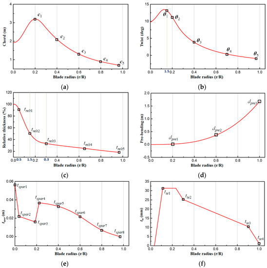
Figure 2.
Definitions of design variables in wind turbine blade design. (a) Chord distribution; (b) Twist distribution; (c) Distribution of relative thickness; (d) Distribution of pre-bending; (e) Distribution of spar cap; (f) Distribution of trailing-edge reinforced layer.
As can be seen in Figure 2a,c, more chord and thickness control point locations are distributed in the blade inboard region, so that the practical dramatic changes in chord and thickness of the blade root can be well represented. The distribution of dpre is fitted using the following exponential function with three variables, as shown in Figure 2d:
where, a, b, c, d, f, g and h are all the coefficients determined through solving linear equation systems resulted from the above equations; R and r represent the blade length and the radial distance from the blade root, respectively.
The main structural components of a wind turbine blade include the skins, spar caps, webs, trailing-edge reinforced layers, and sandwich layers, etc. The materials used in the blade are glass fiber fabric, epoxy resin, polyvinyl chloride (PVC), balsa wood and structural adhesive. Among them, glass fiber fabric and epoxy resin are moulded into composites commonly called the glass fibre reinforced plastics (GFRP). For the 1.5 MW blade, skins are divided into inner skin and outer skin. They not only provide the blade’s aerodynamic shape, but also resist most of the shear load acting on the blade. Thus either biaxial or three-axis glass fiber fabric is used to strengthen the shear resistance ability. Spar caps are employed as the main load bearing units for resisting most of the bending moment, so unidirectional GFRP is used to enhance the strength and stiffness. Webs are mainly used as supporting components for the sustaining spar caps, and also are the shearing-resistance components of blade. A web is composed of two panels and sandwich layer. The panels are made of biaxial GFRP and the sandwich layer is filled with PVC foam. For resisting the flapwise bending moment, trailing-edge reinforced layers are embedded into the blade. Similar to the spar caps, the trailing-edge reinforced layers use unidirectional GFRP, but their thickness and width are obviously smaller than those of the spar caps. A plurality of cavities located at the leading edge and trailing edge regions of the blade are filled with sandwich materials to mainly enhance the blade anti-buckling and anti-instability capability. Along the spanwise direction of the blade, balsa is used near the blade root to further strengthen the anti-buckling capacity and stability owing to its high shear modulus. At the middle and tip of blade, relatively light PVC form is applied to reduce the blade mass.
Based on the above arrangements, the structural design variables of the wind turbine blade must take into account the position, thickness and width of all blade main components mentioned above, together with dozens of key sections used to represent the blade structure, usually resulting in so great number of structural design variables that the blade structure must be simplified on the basis of engineering experience as much as possible for lightening the burden of optimization [30,31]. In this paper, a structure model which is very close to the engineering application is developed for optimizations of the 1.5 MW wind turbine blade. This model is built on the basis of the spar central surface (SCS). SCS is a polynomial-fitting curved surface of the maximum thickness lines of all key blade sections. The position and laminated principle of each component are as follows: the spar cap keeps its width of 420 mm unchanged from the blade root to the tip with varying thickness, and its central line must coincide with the SCS. The thickness distribution of the spar cap (tspar) is selected as design variable. Linear and third-order spline fitting are conducted for the inboard part before the location of the maximum chord length and the part from the location of the maximum chord length to the blade tip, as shown in Figure 2e, where eight variables are defined. The trailing-edge reinforced layer (tte) is made of unidirectional GFRP with the designated width of 120 mm. Five variables are arranged at the designated positions in the spanwise direction of the blade (Figure 2f) and connected to each other in a linear pattern, to determine the thickness distribution of the trailing-edge reinforced layer. The webs are symmetrically placed on both sides of the SCS. The distances between the two webs at the blade root and the blade tip are 300 mm and 120 mm, respectively. The web panels are made of 6-layer biaxial-axis GFRP, while the web sandwich material is PVC form with linear change in thickness from 20 mm at the root to 8 mm at the tip. The blade skins are relatively thin and 2-layer biaxial-axis GFRP are used according to the engineering experience.
2.3. Objective Functions
Four objective functions, which have distinct conflicts, are chosen as optimization goals to investigate the capability of the proposed optimization algorithm [1,14].
2.3.1. Minimum Cost of Energy
Cost of energy (COE), defined as the ratio of the total annual cost to the annual energy production (AEP), is calculated using the model of the NREL cost and scaling mode (NREL CSM) [32,33]. NREL CSM is the most extensively used cost analysis model for wind turbines. It has been applied with high reliability to the cost analysis of several types of wind turbines, ranging from 750 kW to 5 MW [6]. In the model, loads on each component are translated into costs by various pre-constructed empirical cost models. The calculation of the COE is given by:
where TCC represents the turbine capital cost, BOS the balance-of-station costs, and OPEX the operational expenditures; Fr is the financing rate, and β the tax deduction rate.
The annual energy production (AEP) of the wind turbine is mainly determined by wind distribution in a given wind farm and the aerodynamic shape of the blades, including the distributions of chord, twist, thickness and pre-bending. The cost parameters TCC and BOS are determined by the extremely load of wind turbines, so all variables mentioned above are involved for the calculation of the COE.
2.3.2. Maximum AEP
The AEP of the wind turbine is assumed as the primary optimization objective in this study. The AEP under different site conditions can be calculated using the following equation:
where Vin and Vout are the cut-in and cut-out wind speeds. In this study, Vin = 3 m/s and Vout = 25 m/s. Vavg is the annual averaged wind speed, P(V) is the output power at the wind speed V. T is the annual operation hours. f (·) is the Weibull distribution function. According to the design standard of IEC 61400-1, the values of the Weibull shape parameter and Vavg in the wind turbine classes II are 2 and 8.5 m/s.
2.3.3. Minimum Blade Mass
The mass distribution of a blade is calculated based on the classic beam theories. The overall blade mass is then calculated using the following equation:
where Rhub is the hub radius, R the radius of the wind rotor and mi is the mass per unit spanwise length at the i-th section.
In optimization, when the aerodynamic shape and structural layer of a blade, where the variables involved include the chord, twist, relative thickness, absolute thicknesses, spar cap, and trailing-edge reinforced layer, are determined, the laminate theory [34] is used to estimate the mass per unit spanwise length at every blade section.
2.3.4. Minimum Extreme Root Thrust
FAST is used to simulate the aeroelastic responses of the wind turbine. The design load cases (DLCs) are determined according to IEC 61400-1 standard; DLC1.3, DLC1.4, DLC1.5, DLC6.1, and DLC6.3 are used to evaluate the extreme loads, as has been recommended elsewhere [35,36]. The objective function for the minimum extreme root thrust is obtained using the following equation:
where Fx(i) is the root thrust of the i-th DLC.
2.4. Constraints
The chord, twist and relative thickness decrease gradually along the path from the location of maximum chord to the blade tip. The strength and stiffness of the blade are also restricted.
2.4.1. Strength Constraint
The safety factor (SF), defined as the ratio of the maximum stress allowed in the local area (σi) to the stress at the location i (σi), must be greater than one on the entire blade, as in the following:
2.4.2. Deflection Constraint
Deflection of the blade must be controlled to avoid striking the tower. According to IEC 61400-1 standard, the minimum clearance (Dc,min) of the blade should be greater than 30% of the initial clearance (Dc), as in the following:
3. Proposed Algorithm
3.1. Overview of the Algorithm
The procedure of the proposed MODE/D&P algorithm is shown in Figure 3. Uniformly distributed reference vectors are established in the objective space so that populations can approach the PF by surrounding these vectors and eventually converge at the intersection points of these points and PF. In this method, uniformly distributed optimal solutions can be obtained and high performance gradient-based differential evolution algorithm is established to significantly improve optimization efficiency. In contrast to the heuristic searching schemes that are used in conventional GFAs, the proposed algorithm adopts two unique strategies to improve convergence performance and efficiency: (1) a uniform decomposition to maintain population diversity; (2) a neighborhood cross-generation positive-gradient differential evolution with the core of the vectors as the main means to promote population evolution, which dramatically improves the optimization efficiency.
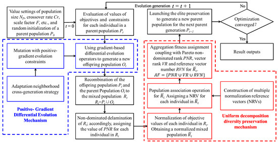
Figure 3.
The MODE/D&P procedure.
3.2. Uniform Decomposition Mechanism for Diversity Preservation
3.2.1. Multiple Normalized Reference Vectors
In MODE/D&P, a series of uniformly distributed reference vectors are set up in the objective space for preserving population diversity [32,37]. These vectors are established in a hyper-cube with a unit size 1, thus are called normalized reference vectors (NRVs), as shown in Figure 4. Anchor points (μi) are fixed at locations on axes with an intercept of 1 and a plane (known as utopia plane) is established by connecting these anchor points. For two- and three-objective optimizations, utopia planes are a straight line (Figure 4) and a regular triangle, respectively. For an optimization over three objectives, utopia plane appears in the form of a simplex hyperplane [38]. Then, utopia points, a set of points located on the utopia plane, are generated by weighting the anchor points using the following equation [38]:
where, m is the number of objectives. The uniformly distributed utopia points can be obtained based on a uniform weighted vector w. In this way, reference vectors, which are a set of lines that are perpendicular to the utopia plane pass through the distributed utopia points, are established. The number of NRVs (NV) can be obtained using the following equation:
where, NS is the number of the divisions of each objective axis; m and C stand for and the combinatorial number, respectively.
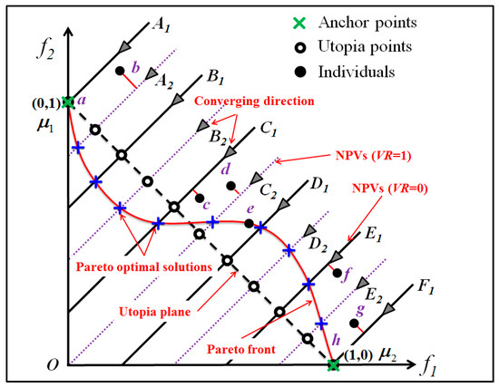
Figure 4.
Schematic of multiple NRVs in double-objective optimization.
NRVs show significant simplex properties (regular triangle) when objective number is more than two, while most PFs in practical optimization cases exhibit complex properties [38]. As a result, a vector may not be linked to one individual of the algorithm while another may be linked to multiple individuals, which can lead to poor algorithm performance and incomplete representation of the PF. In MODE/D&P, the concept of multiple NRVs is introduced to overcome this drawback. For two consecutive ranks of NRVs in two-objective optimization (see Figure 4), NRVs in the second rank (A2, B2, C2, etc.) are obtained by doubling the NS in the first rank (A1, B1, C1, etc.). The vector rank (VR) of each rank is defined as 0 for the first rank and increased by 1 for each successive rank. If necessary, more than two ranks are generated, but each rank is generated only once.
3.2.2. Population Association
The association of populations with NRVs is achieved through three steps. First, the Euclidean distances between each individual and NRVs in the 0th rank are obtained, and the label of the NRV corresponding to the minimum Euclidean distance is considered as a variable of the individual. Then, all the individuals associated with one specific reference vector (j) are categorized in a sub-set. Finally, the individual with the shortest Euclidean distance in each sub-set is selected and the current VR value is attributed to that individual. The other individuals are then associated to the NRVs in the next rank until all the individuals are associated with both a unique vector and the corresponding VR value.
3.2.3. Aggregation Fitness Assignment
The MODE/D&P algorithm involves a fitness distribution operator for the decomposition mechanism, an aggregation fitness assignment [39]. The aggregation fitness assignment consists of the Pareto non-dominated rank (PNR), VR, and reference vector number (RVN). The PNR is achieved through Pareto non-dominated delamination, the VR is generated by the establishment of multiple reference vectors, and the RVN is obtained by population association. The aggregation fitness (AF) of the ith individual is described by:
The AF quantifies its fitness. The AF of an individual decreases as the PNR decreases and with a decrease in the Euclidean distance between the individual and the reference vector that the individual is associated to. This results in an increased probability that the individual will be selected. Additionally, only one unique individual from each sub-set is allowed, which results in good distribution of the population.
3.3. Positive-Gradient Differential Evolution
3.3.1. Neighborhood Cross-Generation Strategy
In classical differential mutations, individuals that are used to establish differential vectors are randomly selected from the current generation. However, the difference in the distributions of two consecutive generations in the objective space in evolution algorithms contains information about converging directions and evolutionary steps of the population, which can be used to conduct rapid searching of individuals.
Based on the widely used “DE/ best/1” mutation scheme in the classic differential evolution [35], a neighborhood cross-generation mutation scheme with vectors as its core is proposed. In the mutation, a sub-population, defined as the neighborhood sub-population (NSP), is developed for each vector that is associated with individuals. The population size (NL) of NSP is set as 5% of the algorithm population size. Then, NL individuals with a minimum Euclidean distance from their associated vector are included in the population. For the ith vector associated with individuals, the two individuals used to establish the differential vector are randomly selected from NSPs in two consecutive generations. The mutation operator of the reference vector i can be modified using the following equations:
where Vi, g is the mutation vector corresponding to the reference vector i, Xi, best, g is the individual associated with the reference vector i, Xi,rn1,g is an individual that is randomly selected from the NSP of the current generation associated with the vector i, Xi,rn2,g−1 is an individual that is randomly selected from the NSP of the previous generation, and F is the scale factor. The subscript g is the generation index. A highly efficient adaptation scheme for the factor F, which has been reported elsewhere, is employed in this study to enhance optimization efficiency of the algorithm [30].
3.3.2. Positive-Gradient Constraints
Ideally, the Pareto optimal solutions are supposed to converge at the intersection points of the reference vectors and the PF (see Figure 5). The most efficient converging pattern is the way that the individuals are continuously approaching the PF along the reference vectors. Therefore, the converging direction is defined as the direction perpendicular to the utopia plane and pointing towards smaller objective values of f1 and f2.
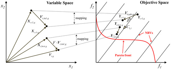
Figure 5.
Relationship of the individuals in the positive-gradient differential evolution.
The positive-gradient constraint is proposed in this study in order to enhance the searching ability of the algorithm. Figure 5 illustrates the relationship among the involved individuals in the positive-gradient differential evolution. The advance vector Vi,adv,g in the objective space is mapped from the trial vector Vi,trial,g in the variable space. If the direction of the advance vector deflects from the converging direction of the reference vector C1,i, it is most likely that the objective values of the reference individual degrade and this evolution fails. Therefore, if the angle β between the advance vector and the positive converging direction is constrained to be below 90 degrees, the positive evolution of the individual has the maximum probability of being guaranteed. In this way, the positive-gradient constraints are established by the following improved formulations:
which satisfies:
where Xi,r1, g and Xi,r2, g are individuals randomly selected from the current generation, and Yi,rn1,g and Yi,rn2,g−1 corresponding to Xi,r1, g and Xi,r2, g−1 are the vectors of the objective values.
4. Results and Discussion
This section presents a series of investigations for the two-, three- and four-objective complex integrated designs of 1.5 MW wind turbine blades based on the proposed MODE/D&P algorithm. For quantitative analyses of the convergence performance and optimization efficiency of the proposed algorithm, the NSGA-II algorithm, which has been widely used in multi-objective designs of wind turbines [11,12], is used as a reference algorithm.
The AeroDyn-1.5MW blade is chosen as a reference blade to provide baseline values to the optimized results. A large amount of validated data of the AeroDyn-1.5MW blade including the geometry, structural layout, aerodynamic performance, mass, load, etc., are available for reference, and detailed data are presented in [40]. In our blade design studies, the rated rotational speed, cut-in speed, cut-out speed, and blade length are 17.4 rpm, 3 m/s, and 25 m/s, 40.3 m, respectively, and blade airfoils are DU and NACA 63 families, consistent with those of the AeroDyn-1.5MW blade. Also, the wind input parameters, the reference wind speed, Weibull wind speed distribution, etc., are set according to the wind turbine class II of IEC 61400-1 [29].
4.1. Design Case Study
4.1.1. Two-Objective Design Case
The objectives of the two-objective design are the minimum COE and maximum AEP, and population size and evolution generation are set to be 20 and 300, respectively.
Figure 6 shows the distributions of Pareto optimal solutions obtained using the MODE/D&P algorithm and the NSGA-II algorithm. The corresponding values of the AeroDyn-1.5MW blade are also included. The distributions of the Pareto optimal solutions follow a monotonically increasing curve, showing that there are conflicts between the two objectives. The approximate uniform distribution of the optimal solutions is achieved using the MODE/D&P algorithm, indicating that the uniform decomposition mechanism of the proposed algorithm is very effective. The optimal solutions obtained using the NSGA-II algorithm exhibited slight aggregation in local areas, as shown in Figure 6b, and does not converge to the approximate PF (indicated by the red line), which is obtained by fitting the optimal solutions from the proposed algorithm using the third order spline, demonstrating inferior convergence performance compared to the proposed algorithm.
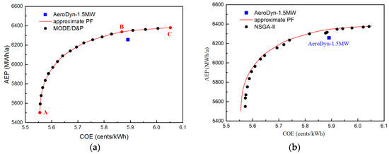
Figure 6.
Optimal solution distributions obtained using the two algorithms in two-objective design. (a) MODE/D&P; (b) NSGA-II.
To explain the reason of the PF formation of wind turbine blade design, the blades A, B and C are selected as samples from Figure 7a for further illustration. Figure 7 shows the distributions of chord, twist, relative thickness, and absolute thickness of Blades A, B, and C based on the optimal solutions obtained using the proposed algorithm, as well as the AeroDyn-1.5MW blade. The power coefficients and extreme flapwise moments of the four blades are given in Figure 8 and Figure 9, respectively. There are two possible reasons for the differences between Blades A and B. First, the AEP of a blade is related to the chord, twist, and relative thickness distributions. The chord of Blade B is larger than that of Blade A, but its relative thickness is relatively smaller. These factors are all beneficial to improve the power output of Blade B, resulting in higher AEP of Blade B. Second, the COE is related to extreme load and AEP. The AEP of Blade C is only 15.1% higher than that of Blade B. The extreme flapwise moment of Blade B is significantly 41.5% higher than that of Blade A due to the larger chord and smaller relative thickness, resulting in significantly increased overall turbine cost. As a result of the contradictory factors mentioned above, the COE of Blade B is obviously larger than that of Blade A. For comparisons between Blades B and C, as well as Blades A and C, the same trends are observed, and therefore such a monotonous increasing curve PF is produced.
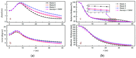
Figure 7.
Distributions of optimal solutions using obtained using the two algorithms in two-objective designs: (a) chord and twist; (b) relative and absolute thicknesses.
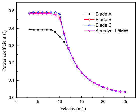
Figure 8.
Comparison of Power coefficients.
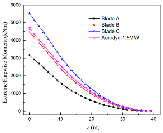
Figure 9.
Comparison of extreme flapwise moments.
The AEP of Blade C is small-amplitude increased 0.7% than that of Blade B, but the COE of Blade C greatly increased 3.1% than Blade B (see Figure 6a). In other words, extreme optimization of a specific objective should not be pursued as it might result in severe performance degradation of the wind turbine in other aspects.
Comparing Blade B with the Aeoydyn-1.5MW blade, the adoption of thinner relative thickness and the reasonable coordination between chord and twist both make the maximum Cp of Blade B reach 0.49, which is higher than that of the reference blade with the maximum value of 0.485. Blade B has smaller chord distribution than the reference does, resulting in lower extreme flapwise moments. The COE of Blade B is lower than that of the reference blade by 3.8%, while the AEP of Blade B is higher than that of the reference by 1.2%, indicating improvements in the both objectives.
4.1.2. Three-Objective Design Case
In the three-objective optimization, the minimum COE, maximum AEP, and minimum blade mass are selected as the optimization objectives. Population size and evolution generation are set at 80 and 500, respectively.
Figure 10 shows the distributions of the optimal solutions obtained using the MODE/D&P and NSGA-II algorithms. The approximate PF is obtained using five-order polynomial fitting. The optimal solutions obtained using the proposed algorithm are uniformly distributed in 3D space, indicating excellent ability of diversity preservation of the proposed algorithm in the three-objective design of the wind turbine. However, severe aggregation of the NSGA-II solutions occurs and, as can be seen, these solutions are distributed in an only approximately curved pattern. Therefore, accurate PF is not achieved in the NSGA-II algorithm, suggesting that the NSGA-II algorithm is the significant deficiency for three-objective designs of wind turbine blade.
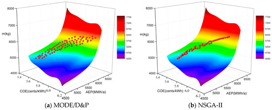
Figure 10.
Pareto optimal solutions obtained using the two algorithms in triple-objective designs. (a) MODE/D&P; (b) NSGA-II.
It should be noted that the curved PF in the three-objective design is influenced by multiple factors, including the chord, twist, relative thickness, absolute thickness, structural layout, and aerodynamic properties and so on. The correlations of these factors are so complicated, which increases the importance of multi-objective design.
4.1.3. Four-Objective Design Case
The objectives of four-objective designs are the minimum COE, maximum AEP, minimum blade mass, and minimum extreme root thrust. The population size and evolution generation are set at 56 and 700, respectively. Only quantitative analysis is conducted here, as the distribution of the Pareto optimal solutions obtained in the four-objective optimization cannot be displayed in 3D space. The Pareto optimal solutions obtained using the MODE/D&P algorithm is given in Figure 11, where the four values are also displayed based on the AerDyn-1.5 MW blade (COE = 5.87 cents/kWh, AEP = 6257 MWh/a, blade mass = 5877 kg, extreme root thrust = 115 kN) for comparison. As can be seen in Figure 11, blades 12, 23, 24, 30, 38, 41 and 44 (in red) exhibit improvements in all objectives compared to the AerDyn-1.5 MW blade and thus are regarded as optimal solutions in this study.
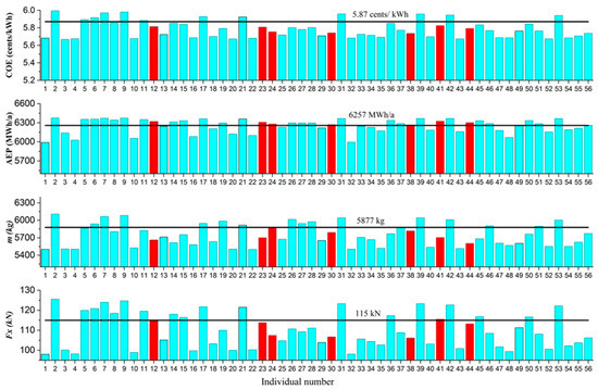
Figure 11.
Pareto optimal solutions obtained using the MODE/D&P algorithm.
4.2. Optimization Efficiency and Convergence
This section presents optimization convergence and efficiency analyses of the proposed algorithm by considering the effects of the number of objective functions and algorithm’s population size. Hyper-volume indicator (IHV), defined as the volume of hyper-cubes in the objective space included in the optimal solutions and the selected reference point [41], is introduced to quantify optimal solutions. IHV is a key indicator for the convergence and distribution of optimal solutions. A high IHV value indicates good approximation to PF and an excellent distribution of the optimal solutions.
4.2.1. Effects of the Number of Optimization Objectives
Figure 12 presents the dimensionless IHV of each evolution process in the two-, three-, and four-objective optimizations using the MODE/D&P and NSGA-II algorithms. As can be seen, the IHV obtained using the MODE/D&P algorithm is significantly higher than that obtained using the NSGA-II algorithm in all the multi-objective optimizations, suggesting that the proposed algorithm is significantly effective in convergence over the NSGA-II algorithm and this superiority increases with the increased number of the optimization objectives.
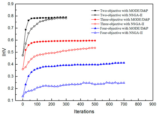
Figure 12.
IHV in two-, three-, and four-objective optimizations using the proposed and NSGA-II algorithms.
The MODE/D&P algorithm also exhibits high efficiency in convergence. It quickly achieves convergence at the 60th and the 80th generation in the two- and three-objective optimizations, respectively. In the four-objective optimization, IHV increases drastically until the 140th generation and then stabilized. Only a slight increase is observed in IHV from the 140th generation to the end of optimization, indicating that convergence is almost achieved. On the contrary, the maximum value of IHV obtained by the NSGA-II algorithm does not reach the IHV at which the proposed algorithm converges, indicating that NSGA-II has very poor efficiency in convergence. Especially in the four-objective optimization, IHV increases slowly with severe fluctuations after the 100th generation in the NSGA-II algorithm. Only a slight increase of IHV is observed at the end of optimization, meaning that the NSGA-II algorithm would fail when the number of optimized objectives is increased.
The main reason for the remarkable difference in performance between the two algorithms is that a series of reference vectors established by uniform decomposition are uniformly distributed in the objective space in the MODE/D&P algorithm, enabling dispersion of populations at early stages of the evolution and reducing the searching range of each individual. Furthermore, cross-generation positive-gradient differential evolution is used to induce a rapid approach of the population towards the PF along reference vectors and a convergence of the population towards the intersection points of the reference vectors and the PF, resulting in excellent optimization efficiency and diversity maintaining capability. Conversely, severe local population aggregations are observed in the NSGA-II algorithm, and most new individuals are in a non-dominant state due to the large number of design variables and the large optimization dimension, leading to poor evolution motivation.
4.2.2. Effects of Population Size
Population size reduction of an evolutionary algorithm is an effective way to improve the optimization efficiency. Based on the three-objective optimization of wind turbine blades, Figure 13 depicts the IHV of 500 generations obtained using the MODE/D&P and NSGA-II algorithms with population sizes of 80, 50 and 20.
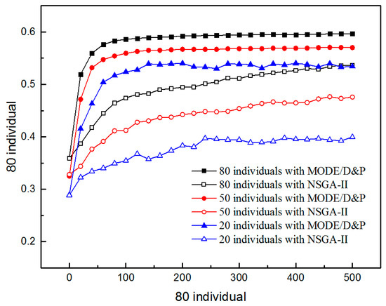
Figure 13.
IHV obtained using the proposed and NSGA-II algorithms with population sizes of 80, 50, and 20.
Convergence is observed in the MODE/D&P algorithm at the 80th and 100th generation at population sizes of 80 and 50, respectively, indicating that the optimization efficiency of the MODE/D&P algorithm decreases with the population size decrease, although the degradation is acceptable. When the population size is 20, the IHV fluctuates after the 140th generation, which can be attributed to the significant effect of individual location on the indicators. Therefore, the population size should be kept a value above a critical level to guarantee reasonable convergence and good efficiency in wind turbine optimization. The optimization efficiency of the NSGA-II algorithm decreases more remarkably with the population size decrease. When the population size is 20, the IHV also fluctuates and is much lower than that of the proposed algorithm. In fact, the values of IHV obtained using the MODE/D&P algorithm are significantly higher than those obtained using the NSGA-II algorithm in all the three cases presented in Figure 13. Therefore, it can be concluded that the MODE/D&P algorithm is more suitable for small population optimization of wind turbine due to its excellent optimization efficiency.
5. Conclusions
A gradient-based multi-objective evolution algorithm is proposed for wind turbine blade design. Uniform decomposition is employed to establish uniformly distributed reference vectors to maintain population diversity so that uniformly distributed Pareto optimal solutions can be obtained. Positive-gradient differential evolution and self-adaptive cross-generation evolution are used to induce a rapid approach of the population towards the PF along the reference vectors and to significantly improve optimization efficiency by reducing the searching ranges of each individual. Two-objective, three-objective, and four-objective optimizations of 1.5 MW wind turbine blades reveal that the proposed algorithm can efficiently provide excellent blade designs. To the best of our knowledge, this is the first time that effective gradient-based methods have been used in multi-objective design of a wind turbine blade and that a uniform decomposition strategy and differential evolution have been combined to develop high performance optimization algorithms.
Compared with [32] this article is an upgraded version, with four significant improvements or differences as follows: (1) Improvements in optimization method. This article not only contains the decomposition mechanism, which is also embodied in the reference article, but also presents a new positive-gradient differential evolution mechanism composing of two operators of the newly proposed positive gradient-constraints and neighborhood cross-generation strategy. The optimization results show that the new algorithm further improves the optimization efficiency by one time compared to the previous algorithm; (2) Improvements in blade modeling. More chord and thickness control point locations in this article are adjusted to be distributed in the blade inboard region, so that the practical dramatic changes in chord and thickness of the blade root can better be represented without deterioration of the whole blade shape description. Moreover, an additional control point is added to the pre-bending description; (3) Differences in optimization objectives. The COE model is introduced to replace the total cost (TC) model used in the previous article. The COE model, representing the rate of investment recovery, is more widely used and more meaningful for wind turbine optimization than the TC model; (4) Differences in the emphasis of the result analysis. Not only are the distributions of optimized solutions analyzed in this article, but also more attentions are paid on the analysis of optimization efficiency and convergence by considering the effects of objective number and algorithm population size.
Author Contributions
All authors were involved during the development of the article. L.W. and T.W. conceived and designed the model setup; L.W. wrote the article and designed the multi-objective optimization algorithm; R.H. wrote the codes to compute power output and cost. S.K. provided valuable insights throughout the research and writing processes.
Acknowledgments
This work was funded by the National Nature science Foundation of China (grant number 51506089, 51506088, and 51761165022), the National Basic Research Program of China (973 Program) (grant number 2014CB046200), and the Priority Academic Program Development of Jiangsu Higher Education Institutions.
Conflicts of Interest
The authors declare no conflict of interest.
References
- Chehouri, A.; Younes, R.; Ilinca, A.; Perron, J. Review of performance optimization techniques applied to wind turbines. Appl. Energy 2015, 142, 361–388. [Google Scholar] [CrossRef]
- Gray, J.S.; Hearn, T.A.; Moore, K.T.; Hwang, J.; Martins, J.; Ning, A. Automatic evaluation of multidisciplinary derivatives using a graph-based problem formulation in Open MDAO. In Proceedings of the 15th AIAA/ISSMO Multidisciplinary Analysis and Optimization Conference, Atlanta, GA, USA, 16–20 June 2014. [Google Scholar]
- Baños, R.; Manzano-Agugliaro, F.; Montoya, F.G.; Gil, C.; Alcayde, A.; Gómez, J. Optimization methods applied to renewable and sustainable energy: A review. Renew. Sustain. Energy Rev. 2011, 15, 1753–1766. [Google Scholar] [CrossRef]
- Chang, B.; Miller, A.; Issa, R.; Chen, G. Review of computer-aided numerical simulation in wind energy. Renew. Sustain. Energy Rev. 2013, 25, 122–134. [Google Scholar]
- Giguère, P.P.; Selig, M.S.; Tangler, J.L. Blade Design Trade-Offs Using Low-Lift Airfoils for Stall-Regulated HAWTs. ASME. J. Sol. Energy Eng. 1999, 121, 217–223. [Google Scholar] [CrossRef][Green Version]
- Benini, E.; Toffolo, A. Optimal Design of Horizontal-Axis Wind Turbines Using Blade-Element Theory and Evolutionary Computation. J. Sol. Energy Eng. 2002, 124, 357–363. [Google Scholar] [CrossRef]
- Kusiak, A.; Zhang, Z.; Li, M. Optimization of Wind Turbine Performance with Data-Driven Models. IEEE Trans. Sustain. Energy 2010, 1, 66–76. [Google Scholar] [CrossRef]
- Dufo, L.R.; Bernal, J.L.; Yusta-Loyo, J.M.; Domínguez-Navarro, J.A.; Ramírez-Rosado, I.J.; Lujanoa, J.; Aso, I. Multi-objective optimization minimizing cost and life cycle emissions of stand-alone PV–wind–diesel systems with batteries storage. Appl. Energy 2011, 88, 4033–4041. [Google Scholar] [CrossRef]
- Ju, Y.P.; Zhang, C.H. Multi-point robust design optimization of wind turbine airfoil under geometric uncertainty. Proc. Inst. Mech. Eng. Part A 2012, 226, 245–261. [Google Scholar] [CrossRef]
- Wang, L.; Wang, T.G.; Luo, Y. Improved non-dominated sorting genetic algorithm (NSGA)-II in multi-objective optimization studies of wind turbine blades. Appl. Math. Mech. 2011, 32, 739–748. [Google Scholar] [CrossRef]
- Sessarego, M.; Dixon, K.R.; Wood, D.E.R.D.H. A hybrid multi-objective evolutionary algorithm for wind-turbine blade optimization. Eng. Opt. 2014, 47, 1–20. [Google Scholar] [CrossRef]
- Sorkhabi, S.Y.D.; Romero, D.A.; Yan, G.K.; Gu, M.D.; Morand, J.; Morgenroth, M.; Amon, C.H. The impact of land use constraints in multi-objective energy-noise wind farm layout optimization. Renew. Energy 2016, 85, 359–370. [Google Scholar] [CrossRef]
- Wang, W.; Caro, S.; Bennis, F.; Soto, R.; Crawford, B. Multi-Objective Robust Optimization Using a Postoptimality Sensitivity Analysis Technique: Application to a Wind Turbine Design. J. Mech. Des. 2015, 137, 1–16. [Google Scholar] [CrossRef]
- Liao, C.C.; Zhao, X.L.; Xu, J.Z. Blade layers optimization of wind turbines using FAST and improved PSO algorithm. Renew. Energy 2012, 42, 227–233. [Google Scholar] [CrossRef]
- Sharafi, M.; Elmekkawy, T.Y.; Bibeau, E.L. Optimal design of hybrid renewable energy systems in buildings with low to high renewable energy ratio. Renew. Energy 2015, 83, 1026–1042. [Google Scholar] [CrossRef]
- Lucken, C.; Baran, B.; Abrizuela, C. A survey on multi-objective evolutionary algorithms for many-objective problems. Comput. Opt. Appl. 2014, 58, 707–756. [Google Scholar]
- Ning, A.; Petch, D. Integrated design of downwind land-based wind turbines using analytic gradients. Wind Energy 2016. [Google Scholar] [CrossRef]
- Wang, X.; Shen, W.Z.; Zhu, W.J.; Sørensen, J.N.; Jin, C. Shape optimization of wind turbine blades. Wind Energy 2009, 12, 781–803. [Google Scholar]
- Wood, D.H. Dual Purpose Design of Small Wind Turbine Blades. Wind Eng. 2004, 28, 511–527. [Google Scholar] [CrossRef]
- Abedi, S.; Alimardani, A.; Gharehpetian, G.B.; Riahy, G.H.; Hosseinian, S.H. A comprehensive method for optimal power management and design of hybrid RES-based autonomous energy systems. Renew. Sustain. Energy Rev. 2012, 16, 1577–1587. [Google Scholar] [CrossRef]
- Wagner, T.; Beume, N.; Naujoks, B. Pareto-, Aggregation-, and Indicator-Based Methods in Many-Objective Optimization // Evolutionary Multi-Criterion Optimization; Springer: Berlin/Heidelberg, Germany, 2007; pp. 742–756. [Google Scholar]
- Hu, Y.; Rao, S.S. Robust Design of Horizontal Axis Wind Turbines Using Taguchi Method. J. Mech. Design 2011, 133, 1543–1548. [Google Scholar] [CrossRef]
- Zhou, A.; Qu, B.Y.; Li, H.; Zhao, S.-Z.; Suganthan, P.N.; Zhang, Q. Multiobjective evolutionary algorithms: A survey of the state of the art. Swarm Evol. Comput. 2011, 1, 32–49. [Google Scholar] [CrossRef]
- Resor, R.B. Definition of a 5 MW/61.5 m Wind Turbine Blade Reference Model; SAND2013-2569 463454; Sandia National Laboratories: Albuquerque, NM, USA, 2013. [Google Scholar]
- Coulling, A.J.; Goupee, A.J.; Robertson, A.N.; Jonkman, J.M.; Dagher, H.J. Validation of a FAST semi-submersible floating wind turbine numerical model with DeepCwind test data. J. Renew. Sustain. Energy 2013, 5, 023116. [Google Scholar] [CrossRef]
- Gasmi, A.; Sprague, M.A.; Jonkman, J.M.; Jones, W.B. Numerical stability and accuracy of temporally coupled multi-physics modules in wind turbine CAE tools. In Proceedings of the AIAA Aerospace Sciences Meeting Including the New Horizons Forum & Aerospace Exposition, Grapevine, TX, USA, 7–10 January 2013. [Google Scholar]
- Jonkman, J.M. Dynamics of offshore floating wind turbines—Model development and verification. Wind Energy 2009, 12, 459–492. [Google Scholar] [CrossRef]
- Jonkman, J.M. Fast Theory Manual; NREL/TP-500-32449; National Renewable Energy Laboratory: Golden, CO, USA, 2013. [Google Scholar]
- International Electrotechnical Commission. Wind Turbines—Part 1: Design Requirements. International Standard, 2005, Reference Number: IEC 61400-1, 3rd ed.; International Electrotechnical Commission: Geneva, Switzerland, 2005. [Google Scholar]
- Monte, A.D.; Castelli, M.R.; Benini, E. Multi-objective structural optimization of a HAWT composite blade. Compos. Struct. 2013, 106, 362–373. [Google Scholar] [CrossRef]
- Chen, X.; Agarwal, R.K. Optimization of Wind Turbine Blade Airfoils Using a Multi-Objective Genetic Algorithm. J. Aircraft 2013, 50, 519–527. [Google Scholar] [CrossRef]
- Wang, L.; Wang, T.; Wu, J.; Chen, G. Multi-objective differential evolution optimization based on uniform decomposition for wind turbine blade design. Energy 2017, 120, 346–361. [Google Scholar] [CrossRef]
- Ning, R.; Damiani, R.; Moriarty, P. Objectives and constraints for wind turbine optimization. J. Sol. Energy Eng. 2013, 136, 303–312. [Google Scholar]
- Bae, S.Y.; Kim, B.-S.; Lee, S.-L.; Kim, Y.-H. Structural Design of Multi-Megawatt Wind Turbine Blade by Classical Lamination Theory. J. Ocean Eng. Technol. 2014, 28, 147–151. [Google Scholar] [CrossRef]
- Qiu, X.; Xu, J.X.; Tan, K.C.; Abbass, H.A. Adaptive Cross-Generation Differential Evolution Operators for Multiobjective Optimization. IEEE Trans. Evol. Comput. 2016, 20, 232–244. [Google Scholar] [CrossRef]
- Fleming, P.A.; Ning, A.; Gebraad, P.M.O.; Dykes, K. Wind plant system engineering through optimization of layout and yaw control. Wind Energy 2016, 19, 329–344. [Google Scholar] [CrossRef]
- Das, I.; Dennis, J.E. Normal-boundary intersection: A new method for generating the Pareto surface in nonlinear multi-criteria optimization problems. Siam J. Opt. 1998, 8, 631–657. [Google Scholar] [CrossRef]
- Messac, A.; Ismail-Yahaya, A.; Mattson, C.A. The normalized normal constraint method for generating the Pareto frontier. Struct. Multidiscip. Opt. 2003, 25, 86–98. [Google Scholar] [CrossRef]
- Wang, L.; Chen, G.P.; Wang, T.G.; Cao, J.F. Numerical Optimization and Noise Analysis of High-Tip-Speed Wind Turbine. Adv. Appl. Math. Mech. 2017, 9, 1461–1484. [Google Scholar] [CrossRef]
- Kremer, V. ae1.5-40.3 Technical Data; Document number: D-18.21-03.00.00.01; Aerodyn Energiesysteme GmbH: Rendsburg, Germany, 2009. [Google Scholar]
- Bader, J.; Zitzler, E. HypE: An algorithm for fast hypervolume-based many-objective optimization. Evol. Comput. 2011, 19, 45–76. [Google Scholar] [CrossRef] [PubMed]


© 2018 by the authors. Licensee MDPI, Basel, Switzerland. This article is an open access article distributed under the terms and conditions of the Creative Commons Attribution (CC BY) license (http://creativecommons.org/licenses/by/4.0/).