Short-Term Forecasting of the Output Power of a Building-Integrated Photovoltaic System Using a Metaheuristic Approach


 ,
,  ,
, 

Abstract
:1. Introduction
2. Related Works
3. Materials and Methods
3.1. Proposed Hybrid DEPSO Forecasting Method
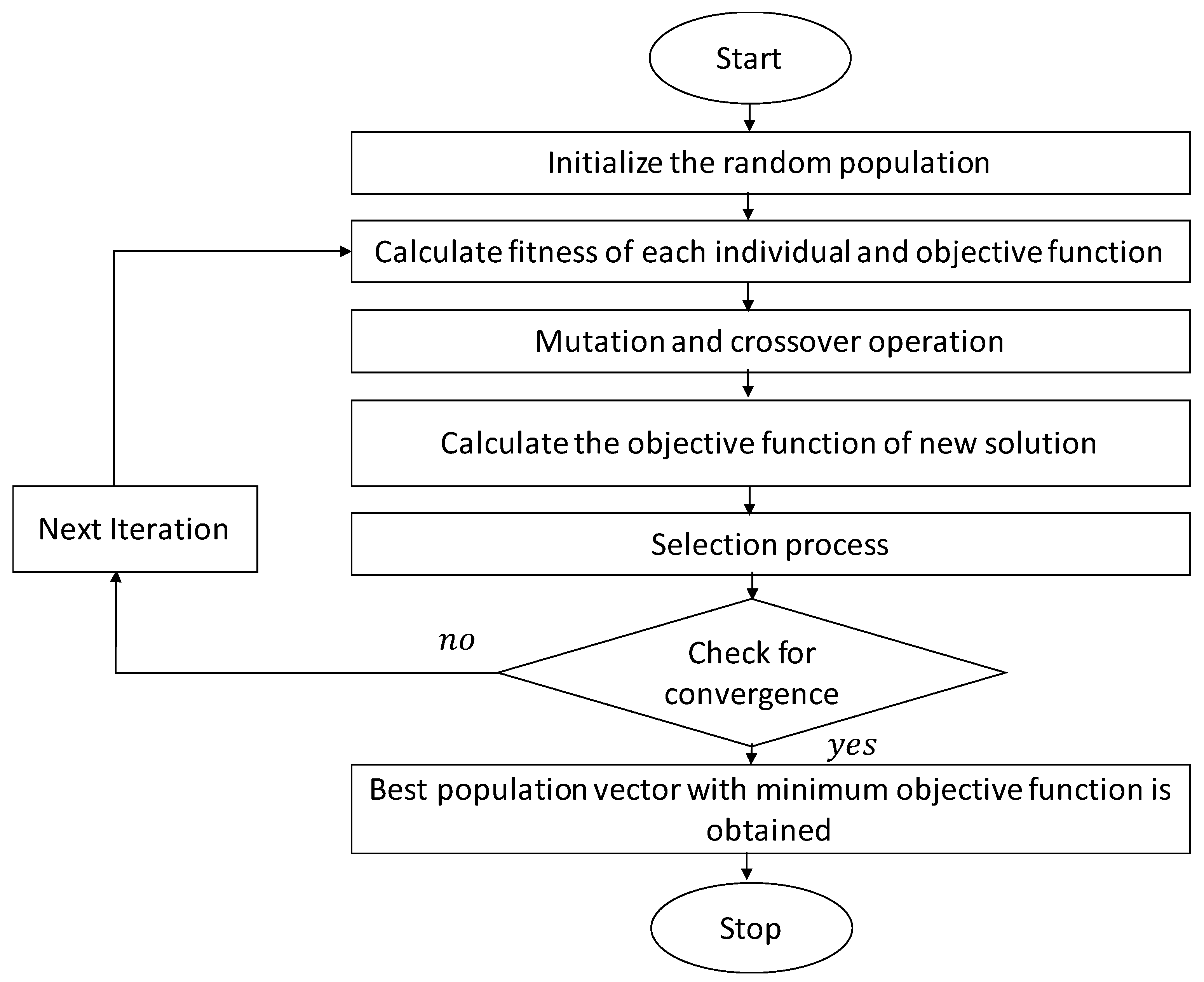
3.1.1. Overview of the DE Algorithm
Theory
Initialization
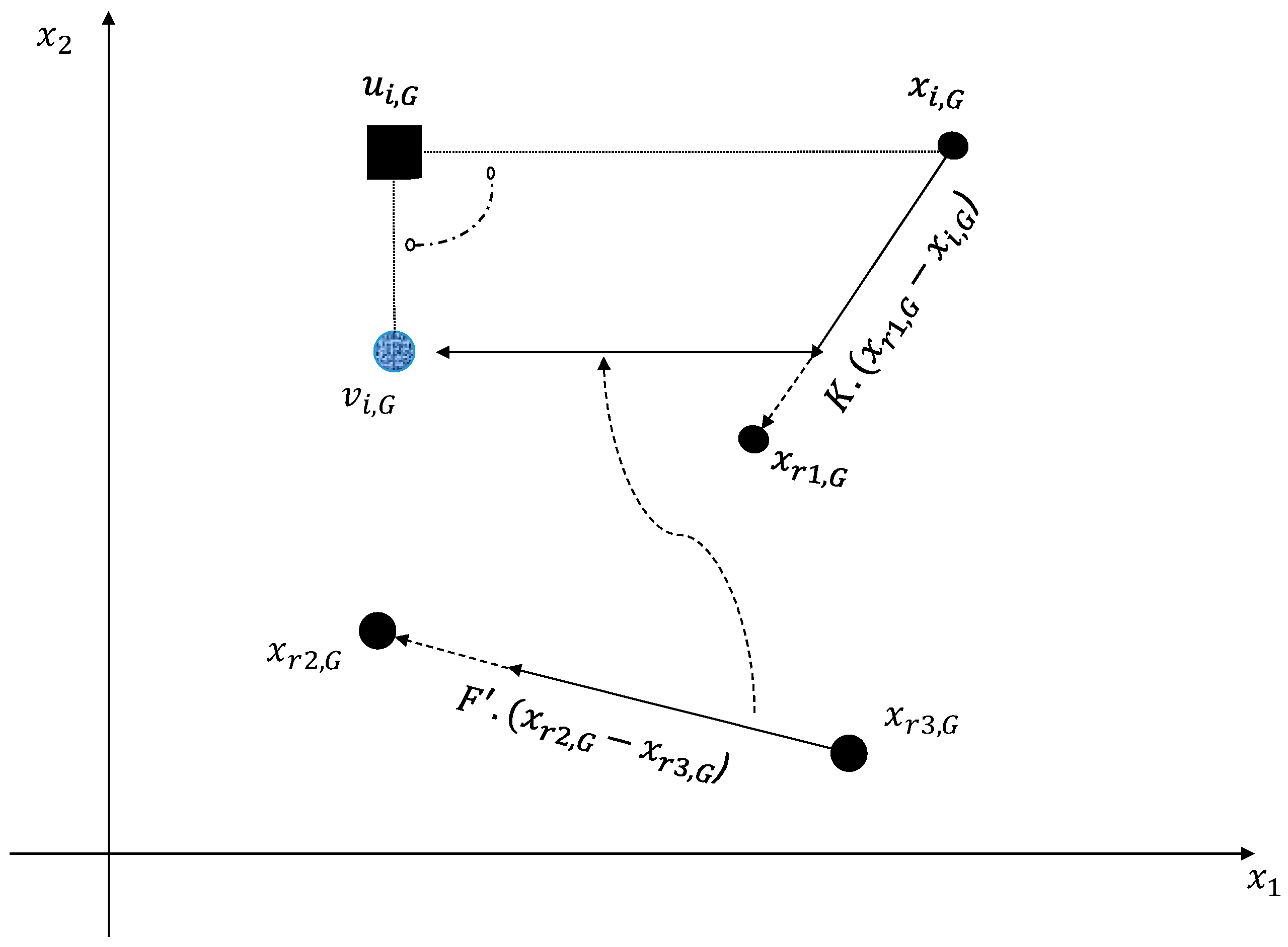
Mutation
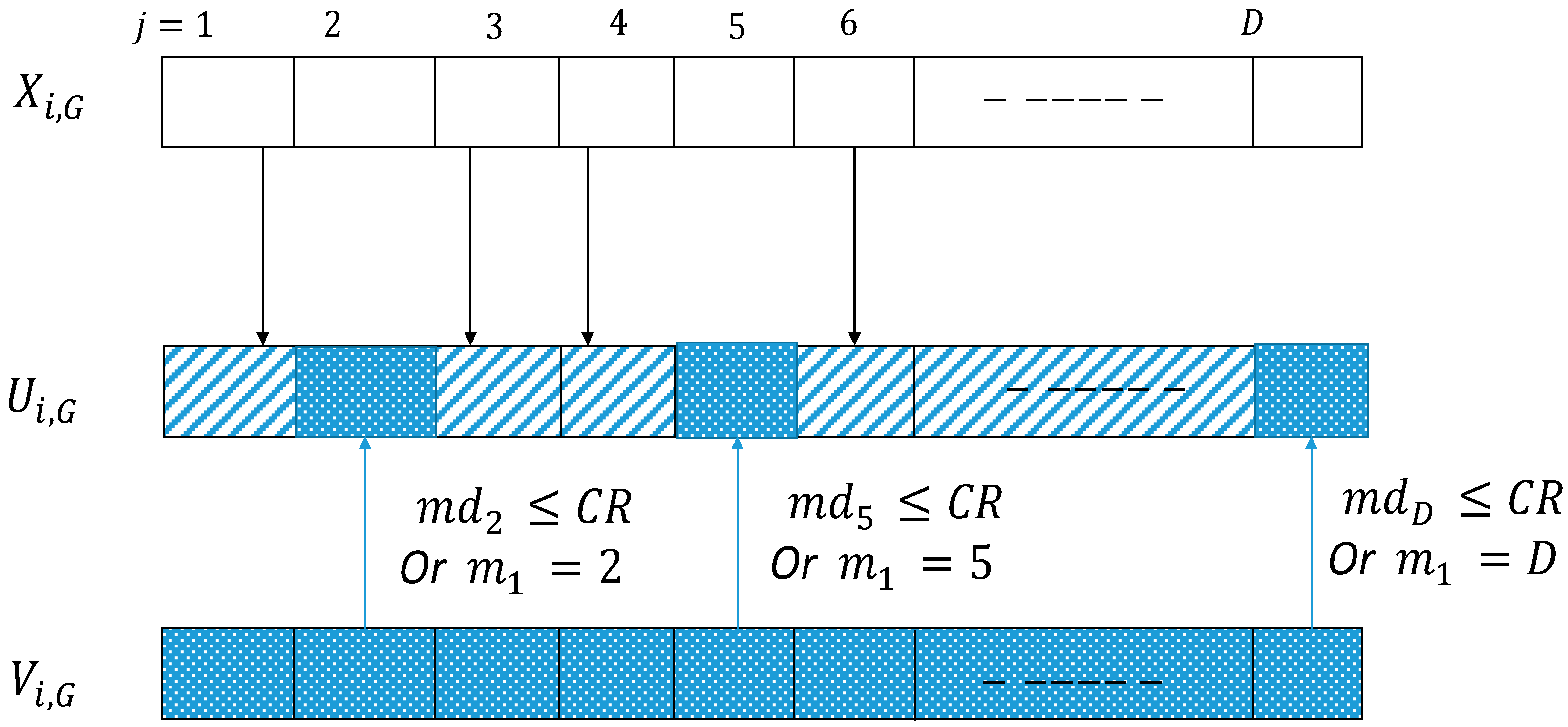
Crossover
Selection
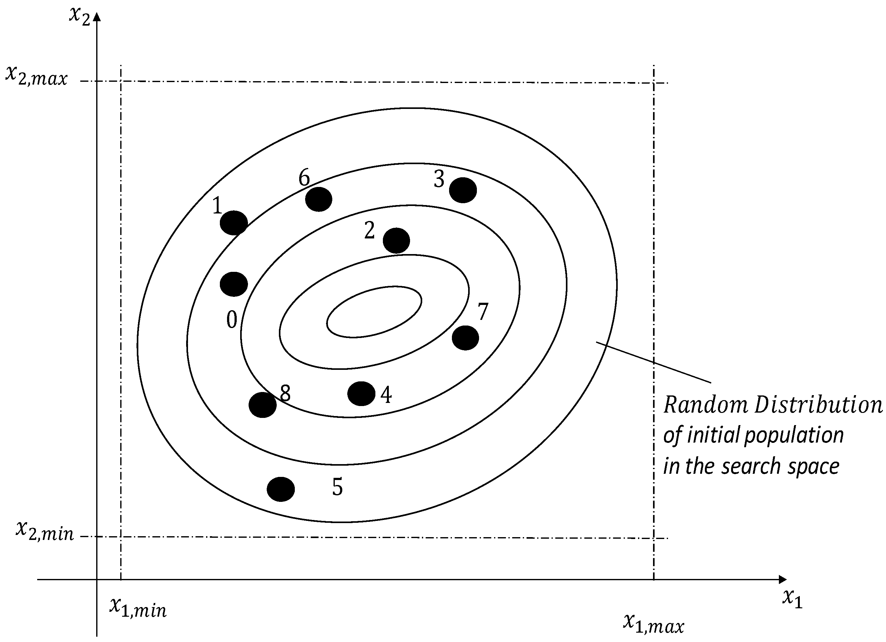
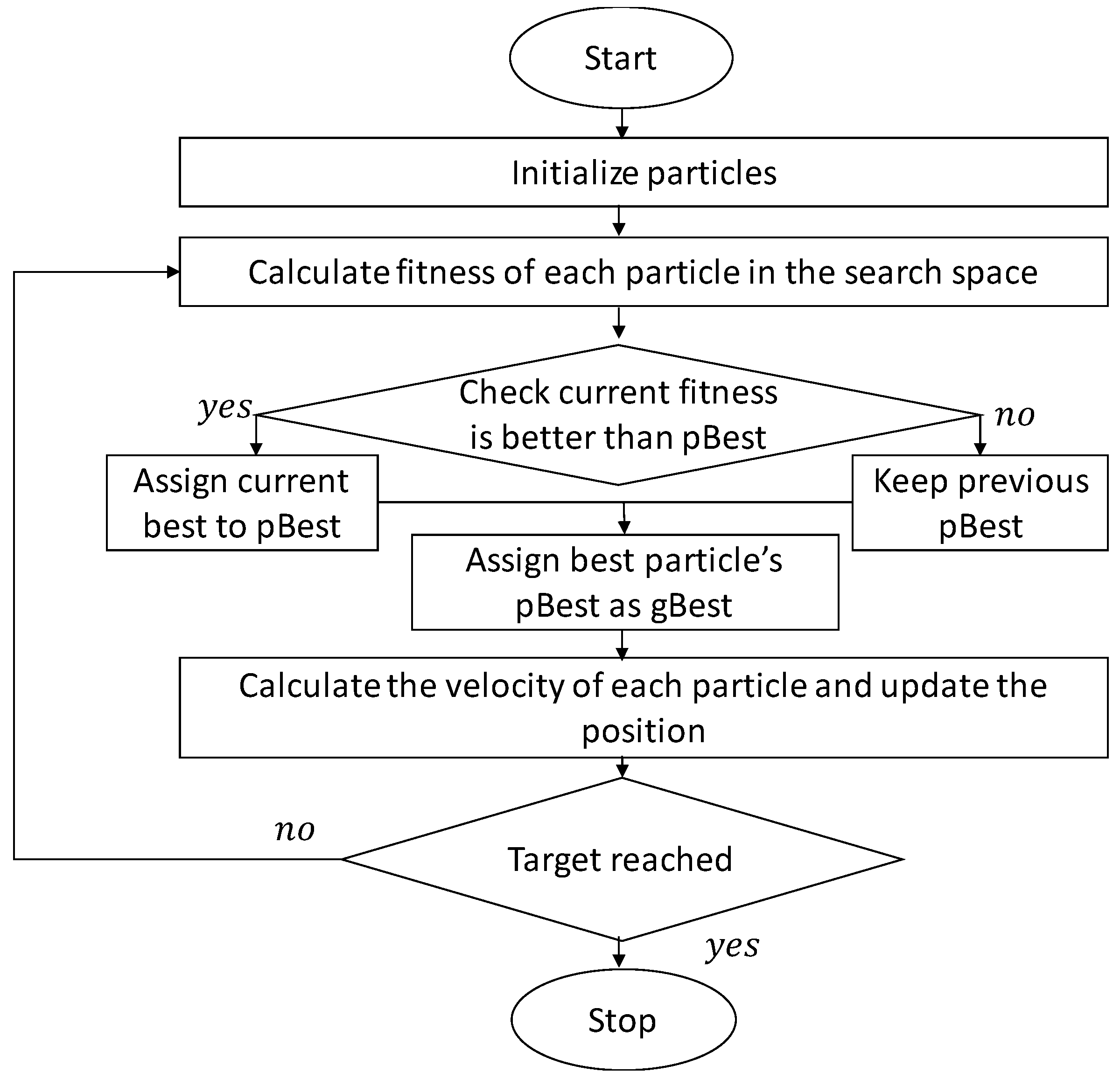
3.1.2. Overview of the PSO Algorithm
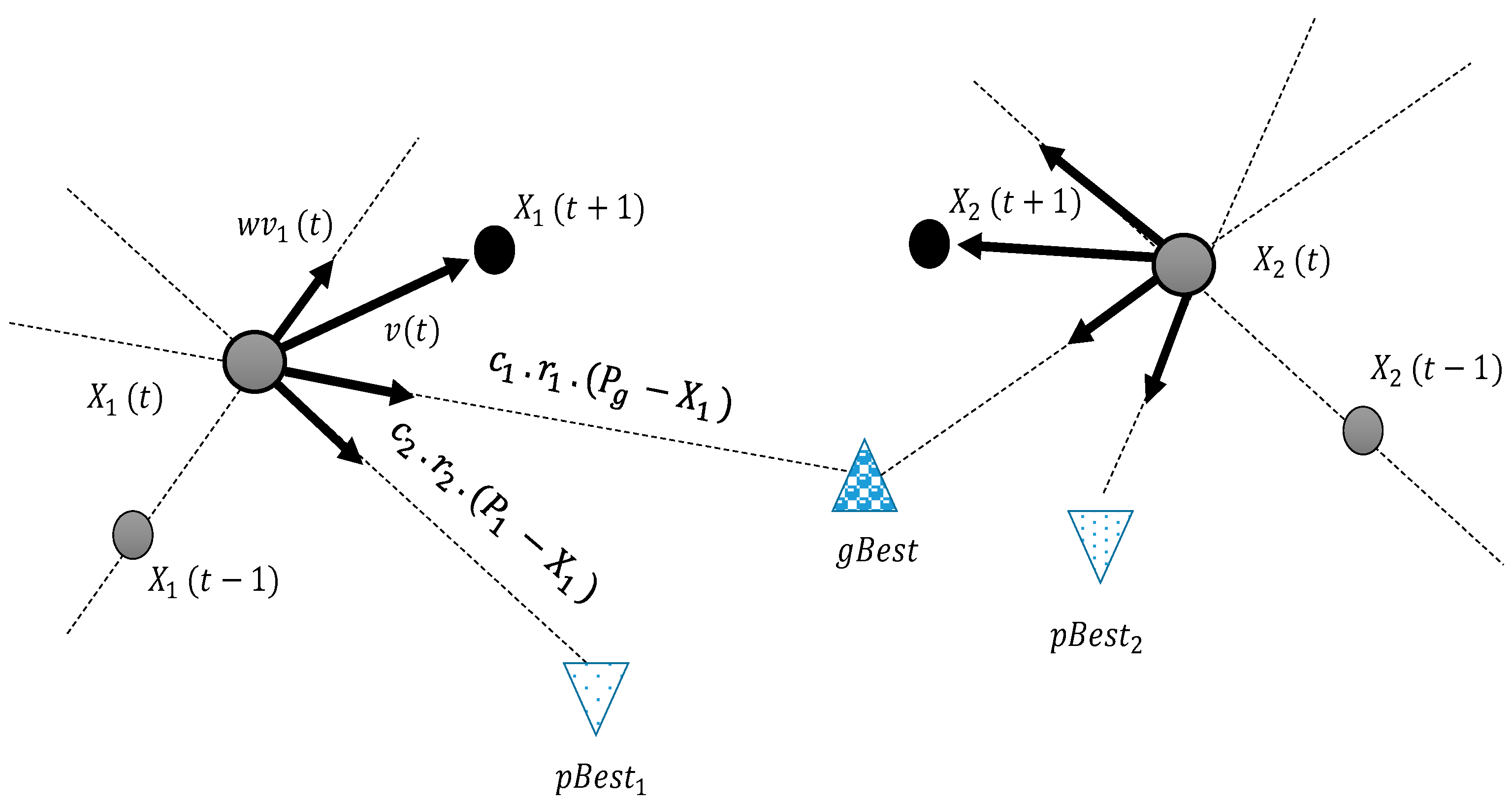
Theory
Initialization
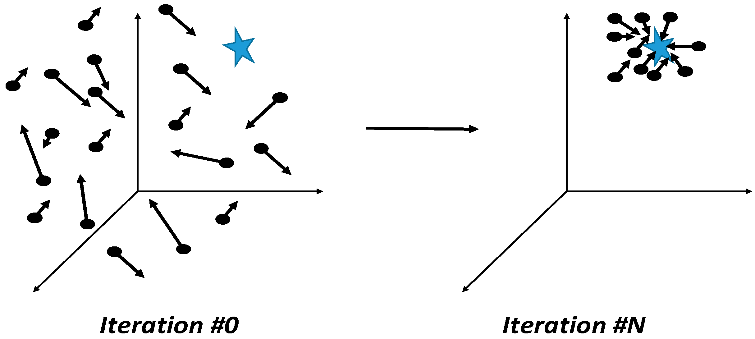
Movement
Evaluation
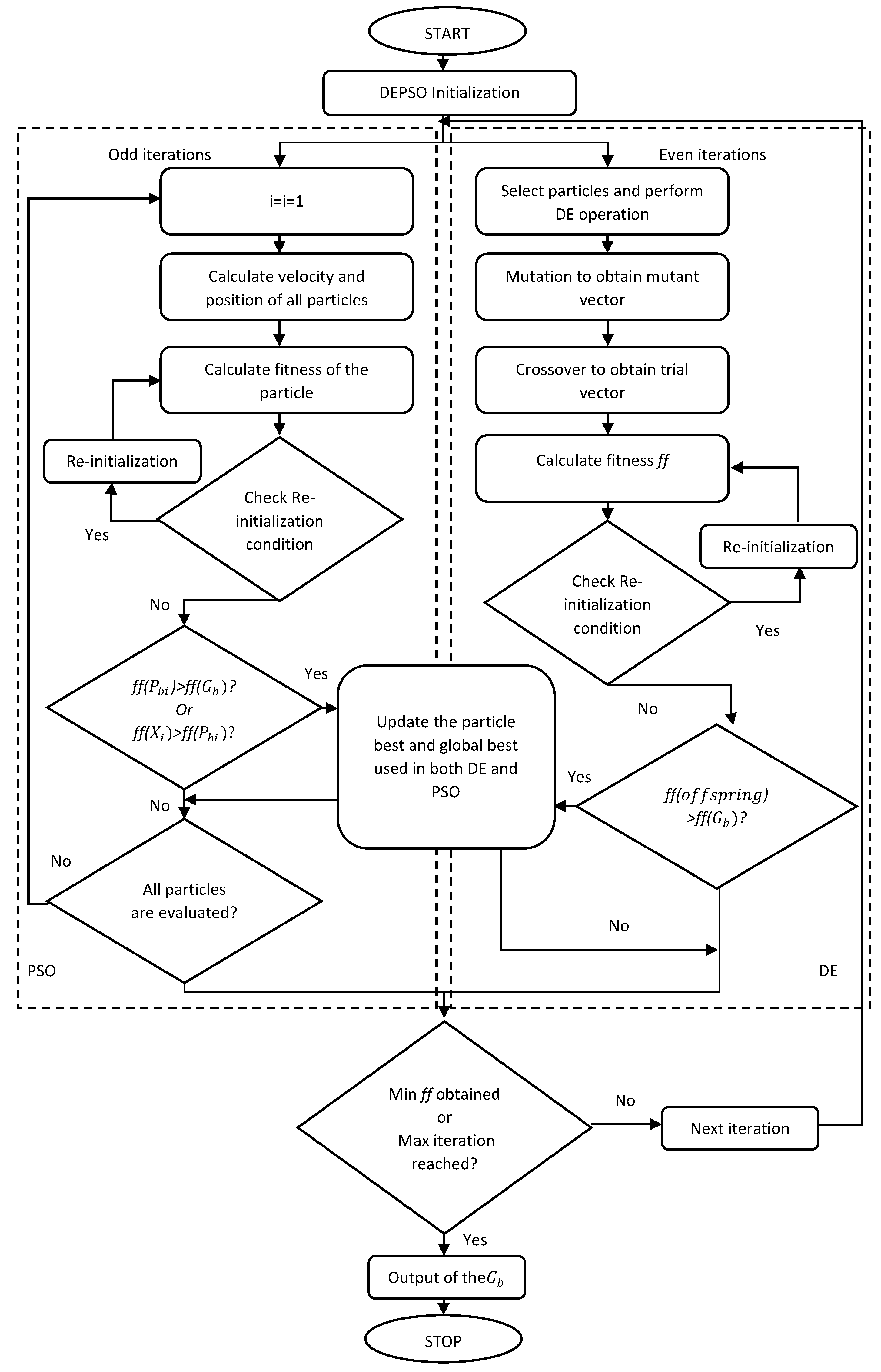
3.1.3. DEPSO Algorithm
3.2. Implementation of DEPSO in Forecasting
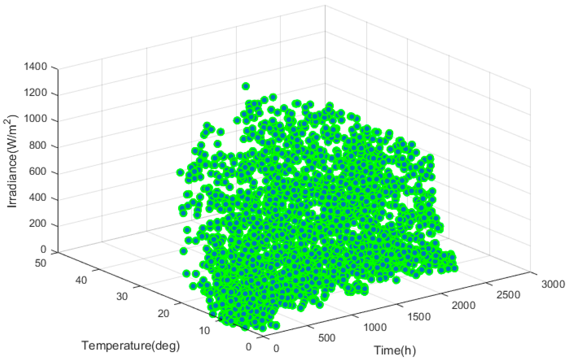
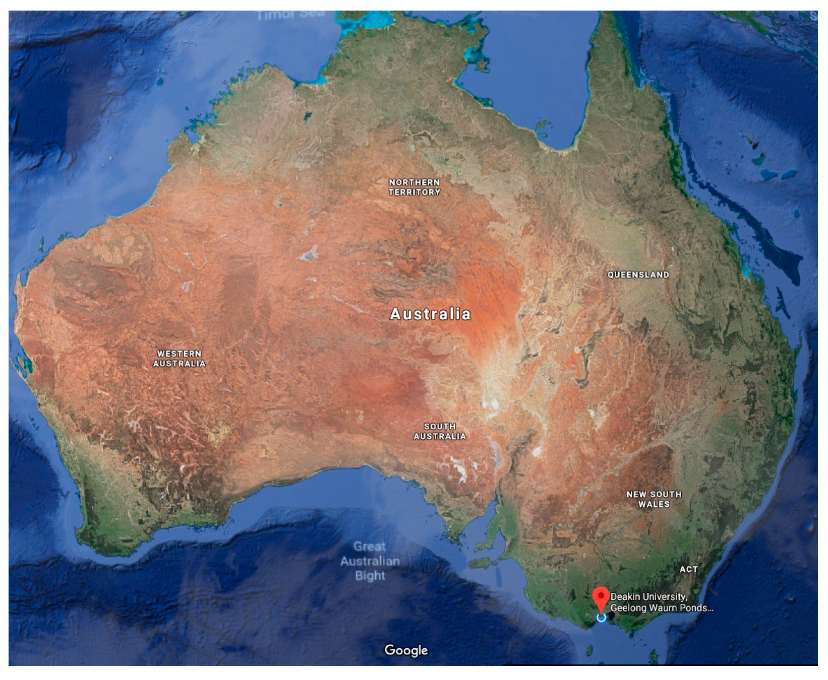
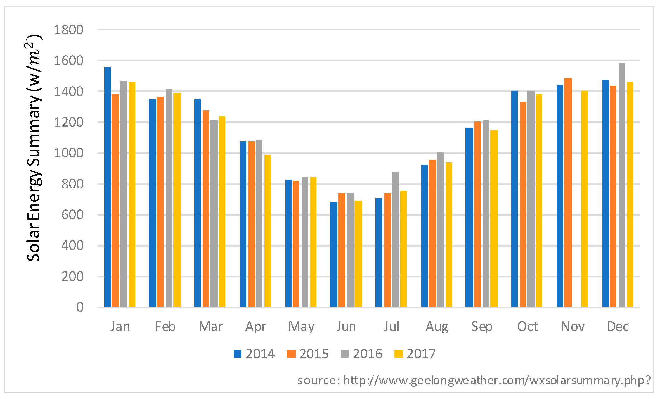
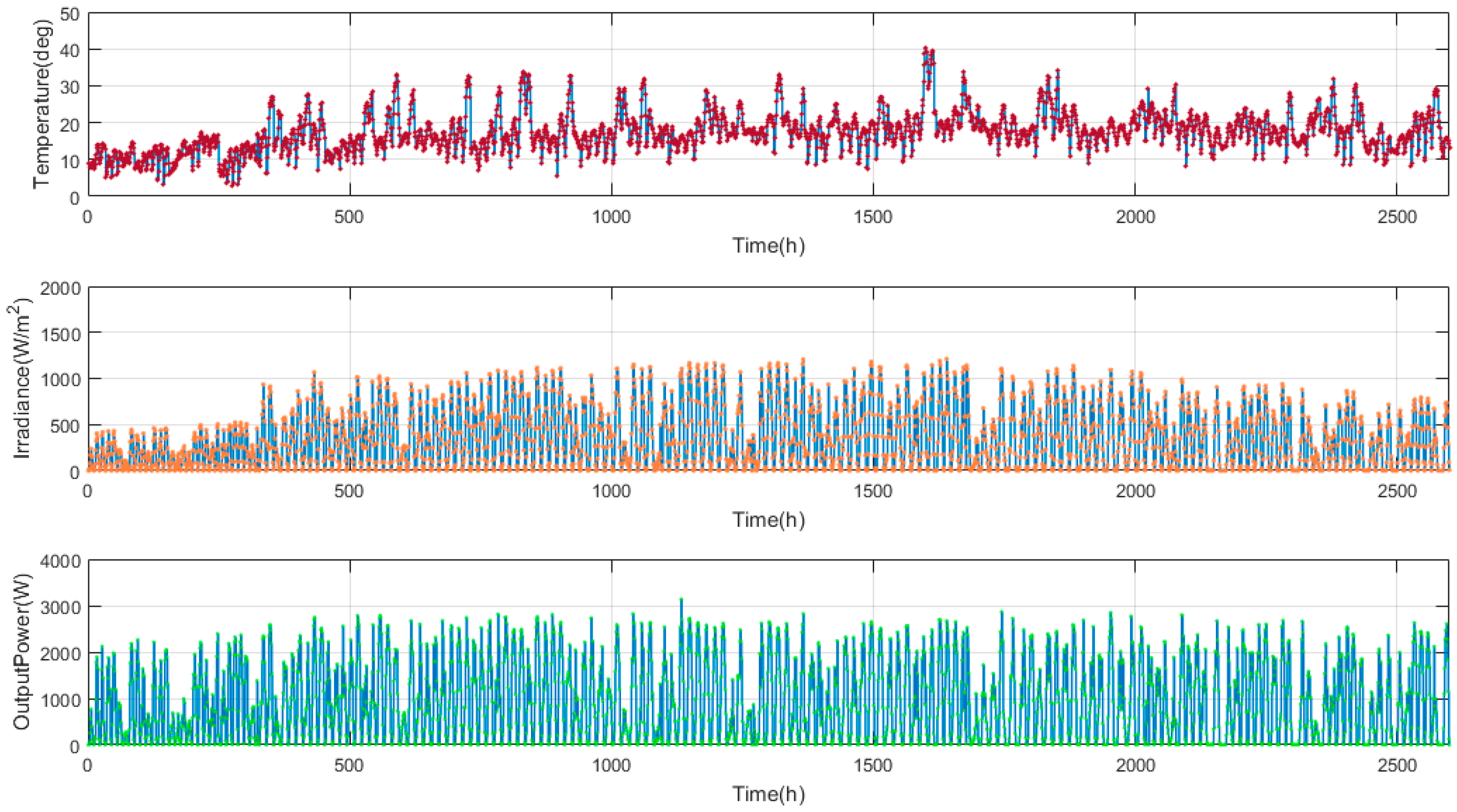
3.3. Data Collection
3.4. Forecast Model
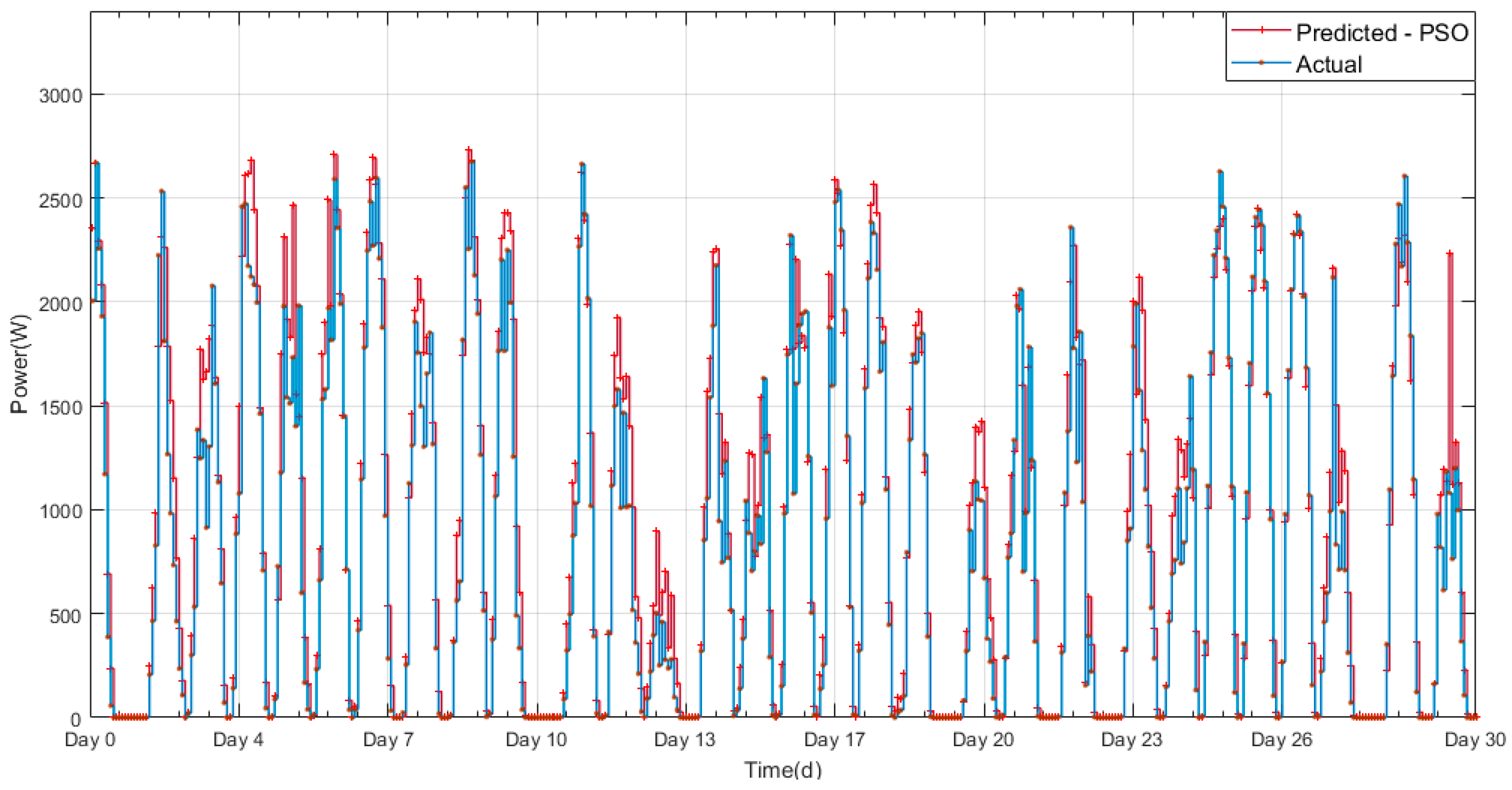
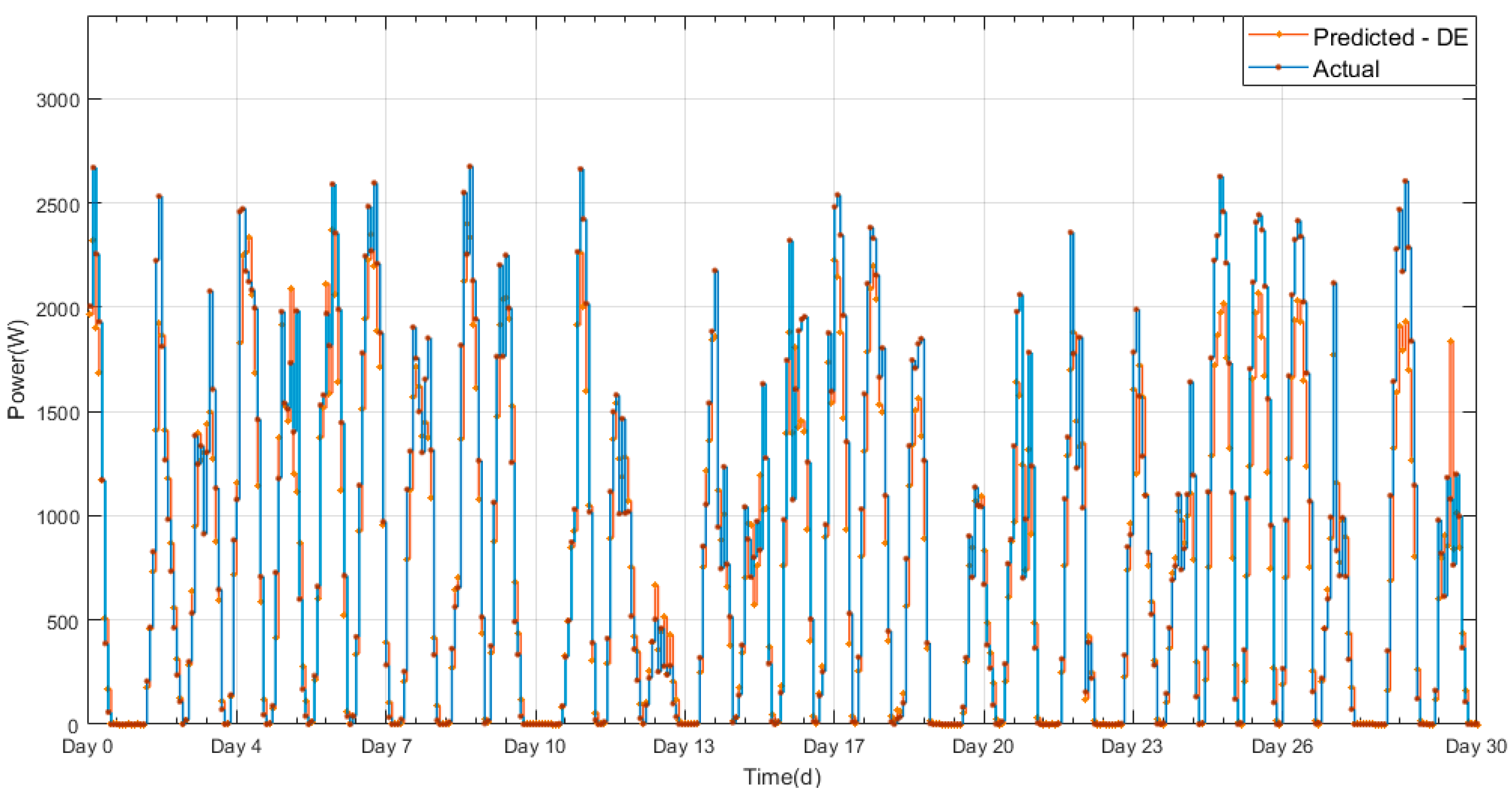
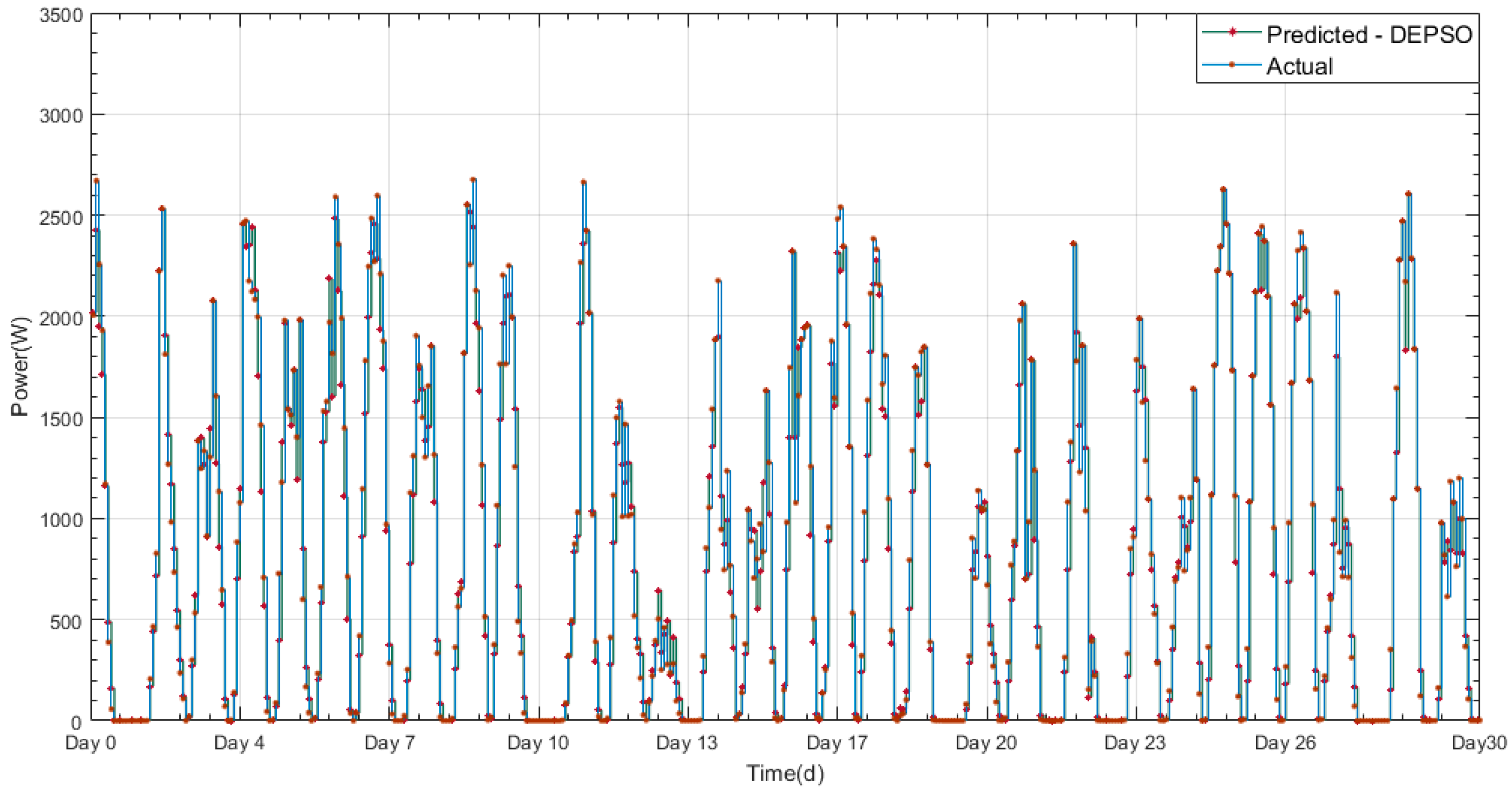
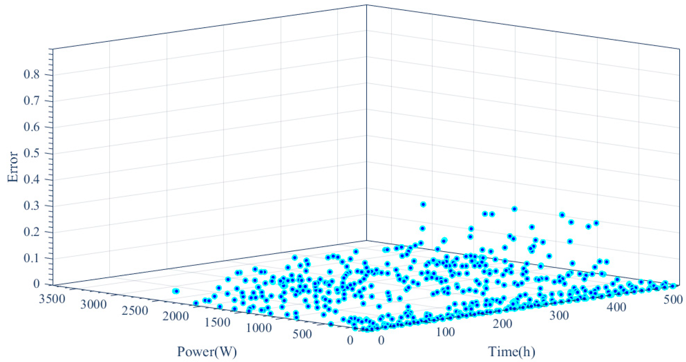
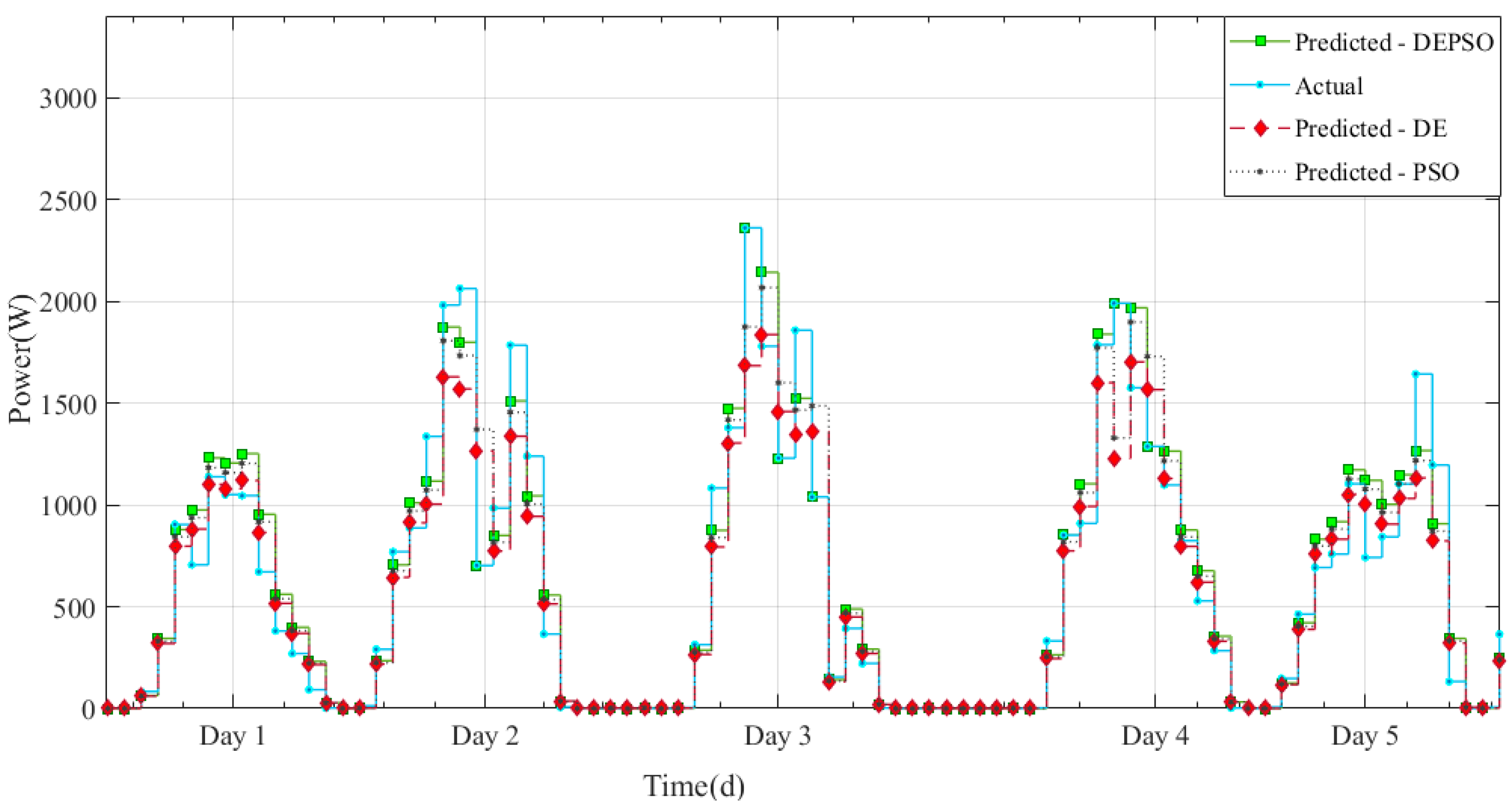
4. Experimental Forecasting Results
5. Conclusions
Author Contributions
Conflicts of Interest
References
- Borchers, A.M.; Duke, J.M.; Parsons, G.R. Does willingness to pay for green energy differ by source? Energy Policy 2007, 35, 3327–3334. [Google Scholar] [CrossRef]
- Panwar, N.L.; Kaushik, S.C.; Kothari, S. Role of renewable energy sources in environmental protection: A review. Renew. Sustain. Energy Rev. 2011, 15, 1513–1524. [Google Scholar] [CrossRef]
- Gillingham, K.; Newell, R.G.; Palmer, K. Energy Efficiency Economics and Policy; National Bureau of Economic Research: Cambridge, MA, USA, 2009. [Google Scholar]
- Boyle, G. Renewable Energy; Oxford University Press: Oxford, UK, 2004. [Google Scholar]
- Lewis, N.S. Toward cost-effective solar energy use. Science 2007, 315, 798–801. [Google Scholar] [CrossRef] [PubMed]
- Baxter, J.; Bian, Z.; Chen, G.; Danielson, D.; Dresselhaus, M.S.; Fedorov, A.G.; Fisher, T.S.; Jones, C.W.; Maginn, E.; et al. Nanoscale design to enable the revolution in renewable energy. Energy Environ. Sci. 2009, 2, 559–588. [Google Scholar] [CrossRef]
- Seyedmahmoudian, M.; Rahmani, R.; Mekhilef, S.; Than Oo, A.M.; Stojcevski, A.; Soon, T.K.; Ghandhari, A.S. Simulation and hardware implementation of new maximum power point tracking technique for partially shaded PV system using hybrid DEPSO method. IEEE Trans. Sustain. Energy 2015, 6, 850–862. [Google Scholar] [CrossRef]
- Cao, S.; Weng, W.; Chen, J.; Liu, W.; Yu, G.; Cao, J. Forecast of Solar Irradiance Using Chaos Optimization Neural Networks. In Proceedings of the 2009 Power and Energy Engineering Conference APPEEC 2009, Asia-Pacific, Wuhan, China, 27–31 October 2009; pp. 1–4. [Google Scholar]
- Liu, J.; Fang, W.; Zhang, X.; Yang, C. An Improved Photovoltaic Power Forecasting Model with the Assistance of Aerosol Index Data. IEEE Trans. Sustain. Energy 2015, 6, 434–442. [Google Scholar] [CrossRef]
- Chen, C.; Duan, S.; Cai, T.; Liu, B. Online 24-h solar power forecasting based on weather type classification using artificial neural network. Sol. Energy 2011, 85, 2856–2870. [Google Scholar] [CrossRef]
- Larson, D.P.; Nonnenmacher, L.; Coimbra, C.F. Day-ahead forecasting of solar power output from photovoltaic plants in the American Southwest. Renew. Energy 2016, 91, 11–20. [Google Scholar] [CrossRef]
- Lusis, P.; Khalilpour, K.R.; Andrew, L.; Liebman, A. Short-term residential load forecasting: Impact of calendar effects and forecast granularity. Appl. Energy 2017, 205, 654–669. [Google Scholar] [CrossRef]
- Seyedmahmoudian, M.; Soon, T.K.; Jamei, E.; Thirunavukkarasu, G.S.; Horan, B.; Mekhilef, S.; Stojcevski, A. Maximum Power Point Tracking for Photovoltaic Systems under Partial Shading Conditions Using Bat Algorithm. Sustainability 2018, 10, 1. [Google Scholar] [CrossRef]
- Wang, F.; Mi, Z.; Su, S.; Zhang, C. A practical model for single-step power prediction of grid-connected PV plant using artificial neural network. In Proceedings of the 2011 IEEE PES Innovative Smart Grid Technologies Asia (ISGT), Perth, WA, Australia, 13–16 November 2011; pp. 1–4. [Google Scholar]
- Shi, J.; Lee, W.-J.; Liu, Y.; Yang, Y.; Wang, P. Forecasting power output of photovoltaic systems based on weather classification and support vector machines. IEEE Trans. Ind. Appl. 2012, 48, 1064–1069. [Google Scholar] [CrossRef]
- Huang, C.-M.T.; Huang, Y.-C.; Huang, K.-Y. A hybrid method for one-day ahead hourly forecasting of PV power output. In Proceedings of the 2014 IEEE 9th Conference on Industrial Electronics and Applications (ICIEA), Hangzhou, China, 9–11 June 2014; pp. 526–531. [Google Scholar]
- Bouzerdoum, M.; Mellit, A.; Pavan, A.M. A hybrid model (SARIMA–SVM) for short-term power forecasting of a small-scale grid-connected photovoltaic plant. Sol. Energy 2013, 98, 226–235. [Google Scholar] [CrossRef]
- Mandal, P.; Madhira, S.T.S.; Meng, J.; Pineda, R.L. Forecasting power output of solar photovoltaic system using wavelet transform and artificial intelligence techniques. Procedia Comput. Sci. 2012, 12, 332–337. [Google Scholar] [CrossRef]
- Cao, J.; Lin, X. Study of hourly and daily solar irradiation forecast using diagonal recurrent wavelet neural networks. Energy Convers. Manag. 2008, 49, 1396–1406. [Google Scholar] [CrossRef]
- Conejo, A.J.; Contreras, J.; Espínola, R.; Plazas, M.A. Forecasting electricity prices for a day-ahead pool-based electric energy market. Int. J. Forecast. 2005, 21, 435–462. [Google Scholar] [CrossRef]
- Antonanzas, J.; Osorio, N.; Escobar, R.; Urraca, R.; Martinez-de-Pison, F.; Antonanzas-Torres, F. Review of photovoltaic power forecasting. Sol. Energy 2016, 136, 78–111. [Google Scholar] [CrossRef]
- Inman, R.H.; Pedro, H.T.C.; Coimbra, C.F.M. Solar forecasting methods for renewable energy integration. Prog. Energy Combustion Sci. 2013, 39, 535–576. [Google Scholar] [CrossRef]
- Uchida, Y.; Tindal, A.; Parkes, J.; Munoz, L. Wind Energy Trading Benefits Through Short Term Forecasting. Proc. Jpn. Wind Energy Symp. 2008, 30, 155–158. [Google Scholar]
- Heinemann, D.; Lorenz, E.; Girodo, M. Forecasting of Solar Radiation, Solar Energy Resource Management for Electricity Generation from Local Level to Global Scale; Nova Science Publisher: New York, NY, USA, 2006. [Google Scholar]
- Grell, G.A.; Dudhia, J.; Stauffer, D.R. A Description of the Fifth-Generation Penn State/NCAR Mesoscale Model (MM5); NCAR: Boulder, CO, USA, 1994. [Google Scholar]
- Done, J.; Davis, C.A.; Weisman, M. The next generation of NWP: Explicit forecasts of convection using the Weather Research and Forecasting (WRF) model. Atmos. Sci. Lett. 2004, 5, 110–117. [Google Scholar] [CrossRef]
- Black, T.L. The new NMC mesoscale Eta model: Description and forecast examples. Weather Forecast. 1994, 9, 265–278. [Google Scholar] [CrossRef]
- Girodo, M. Solarstrahlungsvorhersage auf der Basis numerischer Wettermodelle. Ph. D. Thesis, University of Oldenburg, Oldenburg, Germany, 2006. [Google Scholar]
- Pelland, S.; Galanis, G.; Kallos, G. Solar and photovoltaic forecasting through post-processing of the Global Environmental Multiscale numerical weather prediction model. Prog. Photovolt. Res. Appl. 2013, 21, 284–296. [Google Scholar] [CrossRef]
- Eseye, A.T.; Zhang, J.; Zheng, D.; Li, H.; Jingfu, G. A double-stage hierarchical hybrid PSO-ANN model for short-term wind power prediction. In Proceedings of the 2017 IEEE 2nd International Conference on Cloud Computing and Big Data Analysis (ICCCBDA), Chengdu, China, 28–30 April 2017; pp. 489–493. [Google Scholar]
- Perez, R.; Moore, K.; Wilcox, S.; Renné, D.; Zelenka, A. Forecasting solar radiation–Preliminary evaluation of an approach based upon the national forecast database. Sol. Energy 2007, 81, 809–812. [Google Scholar] [CrossRef]
- Breitkreuz, H.-K. Solare Strahlungsprognosen für energiewirtschaftliche Anwendungen-Der Einfluss von Aerosolen auf das sichtbare Strahlungsangebot. Ph. D. Thesis, Maximilian University of Würzburg, Würzburg, Germany, 2008. [Google Scholar]
- De Giorgi, M.; Congedo, P.; Malvoni, M. Photovoltaic power forecasting using statistical methods: Impact of weather data. IET Sci. Meas. Technol. 2014, 8, 90–97. [Google Scholar] [CrossRef]
- Amjady, N.; Keynia, F.; Zareipour, H. Short-term load forecast of microgrids by a new bilevel prediction strategy. IEEE Trans. Smart Grid 2010, 1, 286–294. [Google Scholar] [CrossRef]
- Pedro, H.T.; Coimbra, C.F. Assessment of forecasting techniques for solar power production with no exogenous inputs. Sol. Energy 2012, 86, 2017–2028. [Google Scholar] [CrossRef]
- Storn, R.; Price, K. Differential Evolution—A Simple and Efficient Heuristic for global Optimization over Continuous Spaces. J. Glob. Optim. 1997, 11, 341–359. (In English) [Google Scholar] [CrossRef]
- Tey, K.S.; Mekhilef, S.; Yang, H.-T.; Chuang, M.-K. A Differential Evolution Based MPPT Method for Photovoltaic Modules under Partial Shading Conditions. Int. J. Photoenergy 2014, 2014, 945906. [Google Scholar] [CrossRef]
- Price, K.V. Differential evolution: A fast and simple numerical optimizer. In Fuzzy Information Processing Society; NAFIPS: Berkeley, CA, USA, 1996; pp. 524–527. [Google Scholar]
- Price, K.V.; Storn, R.M.; Lampinen, J.A. Differential Evolution: A Practical Approach to Global Optimization; Springer: New York, NY, USA, 2005. [Google Scholar]
- Eberhart, R.C.; Kennedy, J. A new optimizer using particle swarm theory. In Proceedings of the Sixth International Symposium on Micro Machine and Human Science, Nagoya, Japan, 4–6 October 1995; IEEE: New York, NY, USA, 1995; Volume 1, pp. 39–43. [Google Scholar]
- Seo, J.H.; Im, C.H.; Heo, C.G.; Kim, J.K.; Jung, H.K.; Lee, C.G. Multimodal function optimization based on particle swarm optimization. IEEE Trans. Magn. 2006, 42, 1095–1098. [Google Scholar] [CrossRef]
- Hao, Z.-F.; Guo, G.-H.; Huang, H. A Particle Swarm Optimization Algorithm with Differential Evolution. In Proceedings of the 2007 International Conference on Machine Learning and Cybernetics, Hongkong, China, 19–22 August 2007; Volume 2, pp. 1031–1035. [Google Scholar]
- Zhang, W.-J.; Xie, X.F. DEPSO: Hybrid particle swarm with differential evolution operator. In Proceedings of the 2003 IEEE International Conference on Systems, Man and Cybernetics, Washington, DC, USA, 5–8 October 2003; Volume 4, pp. 3816–3821. [Google Scholar]
- Moore, P.W.; Venayagamoorthy, G.K. Evolving Digital Circuits Using Hybrid Particle Swarm Optimization and Differential Evolution. Int. J. Neural Syst. 2006, 16, 163–177. [Google Scholar] [CrossRef] [PubMed]
- Rui, X.; Jie, X.; Wunsch, D.C. A Comparison Study of Validity Indices on Swarm-Intelligence-Based Clustering. IEEE Trans. Syst. Man, Cybern. Part B Cybern. 2012, 42, 1243–1256. [Google Scholar] [CrossRef] [PubMed]
- Google Maps. Google Maps. 2018. Available online: https://www.google.com.au/maps/place/Deakin+University,+Geelong+Waurn+Ponds+Campus/@-26.0729556,134.9047233,3651365m/en (accessed on 23 April 2018).
- Ford, W.B. Studies on Divergent Series and Summability, and the Asymptotic Developments of Functions Defined by Maclaurin Series; American Mathematical Soc.: Ann Arbor, MI, USA, 1960. [Google Scholar]
- Kostylev, V.; Pavlovski, A. Solar Power Forecasting Performance—Towards Industry Standards. In Proceedings of the 1st International Workshop on the Integration of Solar Power into Power Systems, Aarhus, Denmark, 24 October 2011. [Google Scholar]


| Ref. | Year of Publication | Method Used | Location | Error Evaluated | Horizon | Training Data |
|---|---|---|---|---|---|---|
| [10] | 2011 | RBF | Online | MAPE, MAE, RMSE | 24 h | 1 year |
| [11] | 2016 | NWP | California, USA | MAE, MBE, RMSE | 1 h, 3 h | 18 months |
| [12] | 2017 | MLR, RT, SVM, NN | New South Wales, Australia | RMSE | 2 h | 3 years |
| [15] | 2012 | SVM | China | RMSE, MRE | 15 m | ~1 year |
| [16] | 2014 | SVR | Taiwan | MRE, RMSE | 1 h | 1 year |
| [18] | 2012 | BPNN, RBFNN, WT + BPNN, WT + RBFNN | Ashland, Oregon | MAPE, MAE, RMSE | 1 h | 30 days |
| [29] | 2013 | NWP | Ontario, Canada | RMSE, MBE, MAE | 48 h | 1 year |
| [30] | 2017 | PSO-ANN, NWP | Beijing, China | MAPE, RMSE, SDE | 1 h | 1 year |
| [33] | 2014 | ANN | Italy | SD, NRMSE, NMAE, NMBE, MSE | 1 h | 1 year |
| [34] | 2010 | GA, PSO, DE, ARIMA, NN, AWINN, | Canada | WME, VAR | 1 day | 4 weeks |
| [35] | 2012 | ARIMA, kNN, ANN, GA/ANN | Merced, California, USA | MAE, MBE, RMSE | 1 h, 2 h | ~2 years |
| C1 | C2 | W | CR | F | K |
|---|---|---|---|---|---|
| 2 | 1.5 | 1.2 | 0.8 | 0.7 | 0.5 |
| Parameter | Value |
|---|---|
| Solar module type | CS6P-250M |
| Number of modules | 12 |
| Module rated power output | 250 W |
| Open circuit voltage () | 37.5 V |
| Short Circuit Current | 8.74 A |
| Optimum operating voltage () | 30.4 V |
| Optimum operating current () | 8.22 A |
| Parameter | Value |
|---|---|
| Number of particles | 100 |
| Number of iterations | 1000 |
| Number of algorithm run | 20 |
| 4.7 × 10⁻⁵ | |
| 3.1 × 10⁻³ | |
| −9.2 × 10⁻³ | |
| 9.4 × 10⁻⁴ | |
| −1.4 × 10⁻³ | |
| 2.5 × 10⁻³ |
| Technique | 1 h | 2 h | 4 h | 1 h | 2 h | 4 h |
|---|---|---|---|---|---|---|
| RMSE (%) | MRE (%) | |||||
| PSO | 14.2 | 15.8 | 21.9 | 9.2 | 11.5 | 13.3 |
| DE | 9.4 | 21.2 | 19.8 | 6.3 | 13.7 | 9.7 |
| DEPSO | 4.4 | 5.2 | 3.5 | 3.1 | 3.17 | 1.6 |
| MAE | MBE | |||||
| PSO | 0.05 | 0.26 | 0.25 | −3.67 | −7.45 | −3.82 |
| DE | 0.06 | 0.23 | 0.19 | −8.25 | −14.25 | −2.15 |
| DEPSO | 0.03 | 0.03 | 0.01 | −1.63 | 5.19 | −1.2 |
| WME | VAR | |||||
| PSO | 0.19 | 0.65 | 0.66 | 0.03 | 0.222 | 0.18 |
| DE | 0.2 | 0.68 | 1.18 | 0.064 | 1.24 | 0.21 |
| DEPSO | 0.16 | 0.28 | 0.16 | 0.01 | 0.79 | 0.12 |
© 2018 by the authors. Licensee MDPI, Basel, Switzerland. This article is an open access article distributed under the terms and conditions of the Creative Commons Attribution (CC BY) license (http://creativecommons.org/licenses/by/4.0/).
Share and Cite
Seyedmahmoudian, M.; Jamei, E.; Thirunavukkarasu, G.S.; Soon, T.K.; Mortimer, M.; Horan, B.; Stojcevski, A.; Mekhilef, S. Short-Term Forecasting of the Output Power of a Building-Integrated Photovoltaic System Using a Metaheuristic Approach. Energies 2018, 11, 1260. https://doi.org/10.3390/en11051260
Seyedmahmoudian M, Jamei E, Thirunavukkarasu GS, Soon TK, Mortimer M, Horan B, Stojcevski A, Mekhilef S. Short-Term Forecasting of the Output Power of a Building-Integrated Photovoltaic System Using a Metaheuristic Approach. Energies. 2018; 11(5):1260. https://doi.org/10.3390/en11051260
Chicago/Turabian StyleSeyedmahmoudian, Mehdi, Elmira Jamei, Gokul Sidarth Thirunavukkarasu, Tey Kok Soon, Michael Mortimer, Ben Horan, Alex Stojcevski, and Saad Mekhilef. 2018. "Short-Term Forecasting of the Output Power of a Building-Integrated Photovoltaic System Using a Metaheuristic Approach" Energies 11, no. 5: 1260. https://doi.org/10.3390/en11051260
APA StyleSeyedmahmoudian, M., Jamei, E., Thirunavukkarasu, G. S., Soon, T. K., Mortimer, M., Horan, B., Stojcevski, A., & Mekhilef, S. (2018). Short-Term Forecasting of the Output Power of a Building-Integrated Photovoltaic System Using a Metaheuristic Approach. Energies, 11(5), 1260. https://doi.org/10.3390/en11051260