Electricity Price Forecasting Using Recurrent Neural Networks

Abstract

Accurate electricity price forecasting has become a substantial requirement since the liberalization of the electricity markets. Due to the challenging nature of electricity prices, which includes high volatility, sharp price spikes and seasonality, various types of electricity price forecasting models still compete and cannot outperform each other consistently. Neural Networks have been successfully used in machine learning problems and Recurrent Neural Networks (RNNs) have been proposed to address time-dependent learning problems. In particular, Long Short Term Memory (LSTM) and Gated Recurrent Units (GRU) are tailor-made for time series price estimation. In this paper, we propose to use multi-layer Gated Recurrent Units as a new technique for electricity price forecasting. We have trained a variety of algorithms with three-year rolling window and compared the results with the RNNs. In our experiments, three-layered GRUs outperformed all other neural network structures and state-of-the-art statistical techniques in a statistically significant manner in the Turkish day-ahead market.

1. Introduction

Since the liberalization of the electricity markets, electricity price forecasting has become an essential task for all the players of the electricity markets for several reasons. Energy supply companies, especially dam-type hydroelectric, natural gas, and fuel oil power plants could optimize their procurement strategies according to the electricity price forecasts. As the share of the regulated electricity markets, such as day-ahead and balancing markets, increase day by day, bilateral contracts also take the market prices as a benchmark [1]. Moreover, prices of the energy derivatives are also based on electricity price forecasts [2]. From the demand side, some companies can schedule their operations according to the low-price zones and operate in these hours or months. Zareipour et al. [3] stressed the importance of the short-term electricity forecasting accuracy. A 1% improvement in the mean absolute percentage error (MAPE) would result in about 0.1–0.35% cost reductions from short term electricity price forecasting [4], which results to circa $1.5 million per year for a medium-size utility with a 5 GW peak load [5].

Electricity prices differ from all other assets and even commodities due to its unique features such as requirement of having constant balance between the supply and demand sides, demand inelasticity, oligopolistic generation side, and non-storability [6]. These features cause some important characteristics of the electricity prices: high volatility, sharp price spikes, mean reverting process, and seasonality in different frequencies [7]. Because of all these idiosyncratic features and characteristics, forecasting the electricity prices accurately becomes a very challenging task.

Machine learning models are able to solve very complicated classification and regression problems with great success. Recently, deep learning models have become the state-of-the-art in speech recognition [8], handwriting recognition [9] and image classification [10].

This paper presents a Gated Recurrent Unit (GRU) based method for electricity price estimation with the goal of using the valuable time series information fully in a neural network architecture. Neural network based methods showed great promise in computer vision, speech recognition and natural language processing [8]. In particular, Recurrent Neural Networks are capable of faithfully preserving the key time-dependent patterns for natural language processing type problems. This motivated us to propose a thorough analysis of multiple features for the electricity prices estimation using Recurrent Neural Networks (RNNs). In particular, the main contributions of this paper are:

• A multi-layer GRU Recurrent Neural Network setup for estimating electricity prices is used.
• A wide analysis of multiple feature settings for neural networks, Convolutional Neural Networks (CNN), Long Short Term Networks (LSTM) and state-of-the-art statistical methods is performed.
• Extensive electricity price estimation performance analysis with both daily and monthly comparisons is made.
• Detailed analysis between the state-of-the-art statistical models and the neural network based methods is made.

1.1. Literature

Electricity price forecasting literature started to develop in the beginning of the 2000s [11,12,13,14,15,16,17]. Following the review by Weron [18], we partition the main methods of electricity price forecasting into five groups: multi-agent, fundamental, reduced-form, statistical, and computational intelligence models.

Multi-agent models simulate the operation of the system and build the price process by matching the demand and the supply. The papers by Shafie-Khah et al. [19] and Ziel and Steinert [20] are very good and recent examples of these type of papers. Shafie-Khah et al. [19] modelled wind power producers, plug-in electricity vehicle owners and customers, who participated into demand response programs, as independent agents in a small Spanish market. Furthermore, Ziel and Steinert [20] proposed a model for the German European Power Exchange (EPEX) market, which considers all the supply and demand information of the system and discusses the effects of the changes in supply and demand.

Fundamental or structural methods discuss the effects of the physical and economic factors on the electricity prices. In this part of the literature, variables are modelled and predicted independently, often via other methods such as reduced-form, statistical or machine learning methods. For example, Howison and Coulon [21] developed a model for electricity spot prices using the stochastic processes of the independent variables. Their method also takes the bid stack function of the price drivers and the electricity prices into account. In another study, Carmona and Coulon [22] focused on the role of the energy prices and effect of the fundamental factors on the electricity prices in a survey about the structural methods. Carmona et al. [22] also discussed the superiority of the fundamental models to the reduced-form models. Both Carmona and Coulon [2] and Füss et al. [23] constructed fundamental models to achieve the final aim of electricity derivatives pricing.

Reduced-form models mainly consist of two methods: Markov regime-switching and jump diffusion. These models are relatively better than structural and statistical models in terms of handling spikes. Geman and Roncoroni [24] used mean-reverting jump diffusion (MRJD) model. Their approach captures both trajectory and statistical components of the electricity prices. Cartea and Figueroa [25] and Janczura et al. [26] used more hybrid methods. First, theyed filter out the jumps using a jump diffusion model and then they proposed more statistical methods to model the remaining, stationary part of the series. Hayfavi and Talasli [7] applied a hybrid-jump diffusion model to the Turkish market and compared the results with [25,27]. Janczura and Weron [27] compared some of the examples in the literature with their own three-regime-switching Markov model, which captures both positive and negative spikes, in addition to exhibiting the inverse leverage effect of the electricity spot prices. Furthermore, Eichler and Türk [28] proposed a semi-parametric Markov regime-switching model. In their method, model parameters are employed by robust statistical techniques. Moreover, it is easier to estimate, and needs less computational time and distributional assumptions. Keles et al. [29] and Bordignon et al. [30] used jump diffusion and Markov regime-switching, respectively, in hybrid works.

Statistical and computational intelligence are the most common models in the electricity price forecasting literature. Statistical models are in great variety from basic naive method [14] to very developed methods [31]. As Ziel and Weron [31] discussed, there are univariate and multivariate frameworks in the electricity price forecasting. In day-ahead electricity price forecasting, players bid the prices and the quantities for the 24 h of the next day. In this sense, the first way is to predict all the prices in a univariate framework from a single price series as a 24-step-ahead forecast. Forecasting the prices from 24 different time series as one-step-ahead forecasts is another option, which is called multivariate framework. Weron and Misiorek [32] applied the univariate framework to the Nordic data. Kristiansen [33] utilized the multivariate framework on the same dataset in a follow-up study and argued that using univariate framework increases the prediction accuracy. However, it contradicts with the findings of Cuaresma [16], who mentioned that using the multivariate framework presents better forecasting results than univariate method. In the same Nordpool market, Raviv et al. [34] have a different point of view. It compares the one-step-ahead daily average price forecasts in a univariate framework with the aggregated 24-step-ahead forecasts of the hourly prices. From empirical evidence, Raviv et al. [34] stated that multivariate framework has lower out-of-sample errors than the univariate one. Nogales et al. [14], Contreras et al. [13], and Conejo et al. [35] presented some substantial examples of the auto-regressive models. Nogales et al. [14] proposed the naive method and, as mentioned by Contreras et al. [13], Nogales et al. [14] and Conejo et al. [35], poorly-calibrated forecasting methods cannot outperform the naive method. Although Conejo et al. [35] found that Auto-regressive Integrated Moving Average (ARIMA) model is worse than the model with exogenous variables in the American PJM market, Contreras et al. [13] stated that adding an exogenous variable does not necessarily increase the prediction accuracy.

Many types of computational intelligence models are applied in the electricity price forecasting literature. Some of the early stage papers were presented by Mandal et al. [36], Catalão et al. [37] and Zhang and Cheng [38]. Mandal et al. [36] forecasted the electricity loads and prices in the Australian market by applying Artificial Neural Network (ANN) model for 1–6 h ahead. MAPE increased from 9.75% to 20.03% when one-step ahead forecast increased to six-step ahead forecast. In another study, Catalao et al. [37] utilized a three-layered feed-forward neural network, which is trained by Levenberg–Marquardt method, and forecasted 168-step-ahead in the Spanish and Californian markets. Although they gave the results for all the seasons of the Spanish market, in the Californian market, results are available only for the Spring term. Therefore, it is difficult to compare the results of both markets. Differently, Zhang and Cheng [38] forecasted the daily average prices and required only one-step-ahead forecast. In the Nordpool market, a standard error back-propagation method is used, which is improved by self-adaptive learning rate and momentum coefficient algorithms. Results indicate that ANN model outperforms the standard ARIMA method. Recent studies by Keles et al. [1] and Panapakidis and Dagoumas [39] apply mainly ANN methods. Keles et al. [1] proposed ANN models with different variables by utilizing the clustering methods. Their ANN based method outperforms the benchmark naive-type models and the Seasonal Auto-regressive Integrated Moving Average (SARIMA) model. An important contribution of this work is the thorough analysis of the forecast accuracy according to the months, extreme price levels, and small and extreme price changes. Panapakidis and Dagoumas [39] compared the forecast performances of different ANN models with various numbers of variables, layers and neurons. The main approach they applied is the clustering of the groups. According to their results, clustering gives 20% better results. Amjady et al. [40] applied fuzzy neural network, Zhao et al. [41] performed support vector machines, Alamaniotis et al. [42] used kernel machines and Pindoriya et al. [43] utilized adaptive wavelet-neural network.

1.2. Turkish Market

Electricity markets differ from country to country for several reasons. The main difference is the supply share of different production methods. When share of renewables, i.e., wind and solar, as well as hydro power plants increase, prices tend to decrease. As Diaz and Planas [44] mentioned, Spanish market has many zeros, which is the minimum price allowed, as well as in the Canadian market [45]. Turkish market has the same price floor of 0 and the price cap of 2000 Turkish Liras/MWh (about 598 Euros/MWh, by the 2016 average exchange rate). Furthermore, as Fanone et al. [46] and Keles et al. [29] mentioned, many negative prices occur due to increased wind share in the German market and it needs special attention. Ugurlu et al. [6] mentioned some information about the shares of the installed capacity in the Turkish market: 34.2% for hydro and 7.6% for wind. In addition to the improved technology in the other supply methods, increasing shares of hydro and wind trigger the decrease in the Turkish day-ahead market electricity prices, which causes many zeros in the price series. These zeros require a special treatment and transformation prior the forecasting procedure [6,44,47]. Avci-Surucu et al. [48] and Ozozen et al. [49] gave some information about the working mechanism of the Turkish day-ahead market. Day-ahead market is used to balance the electricity requirement one day before the physical delivery of the electricity [6]. As in many other markets, market participants give their bids in terms of quantity and price until 11:00, and the price for each hour of the next day is determined by the market maker until 14:00 according to the intersection of the supply and demand curves. It is aimed to meet the required demand with the lowest possible price.

Turkish day-ahead electricity market has an improving literature. Hayfavi and Talasli [7] reported one of the first works, which proposes a multifactor model and compares the model with [25,27]. The stochastic model composed of three jump processes outperforms [25,27] according to the comparison of the empirical moments and model moments in the daily Turkish data. Kolmek and Navruz [50] compared an artificial neural network (ANN) model with the ARIMA model. According to their results, performance of the models differ widely in respect to the selected evaluation period. However, overall, ANN model is a little better than the ARIMA model. In another work, Ozguner et al. [51] proposed an ANN model to forecast the hourly electricity prices and loads in the Turkish market and compared the results with multiple linear regression. Findings of this paper is very similar to [50]; in both papers, ANN model outperforms ARIMA model with a small difference. Ozyildirim and Beyazit [52] compared another machine learning method, radial basis function, with the multiple linear regression. In their work, difference between the prediction performance of the models are negligible. [49] adapted a method from the literature to Turkish electricity prices and takes the residuals of the SARIMA forecast and puts it into ANN procedure. However; the simple model of Ugurlu et al. [6], which even does not include an exogenous variable, outperforms [49]. In our opinion, the reason for the better performance is the factorial Analysis of Variance (ANOVA) application of [6] on the electricity price series prior to forecasting. Although the best model varies from period to period, SARIMA is chosen as the best statistical model for the Turkish day-ahead market in [6].

1.3. Deep Learning

Neural networks transform into deep neural networks (deep learning) with the addition of more layers into the neural network mechanisms. Besides, recurrent neural networks such as LSTM and GRU have started to give better results in the time series data, which triggered the application of these methods in the electricity price forecasting and related literature. RNNs have shown great success in speech recognition, handwriting recognition and polyphonic music modelling [8]. In the electricity load forecasting literature, Zheng et al. [53] applied similar days selection and empirical mode decomposition methods in addition to LSTM, and their method outperforms many state-of-the-art methods such as support vector regression, ARIMA or ANN. Xiaoyun et al. [54] made wind power forecast by combining principal component analysis (PCA) with LSTM. In a solar power forecast research, Gensler et al. [55] applied LSTM method with AutoEncoder and the results show that LSTM usage gives much better results than ANN. In another work, Bao et al. [56] applied very similar method to the stock price forecasting and used wavelet transformation, stacked AutoEncoders and LSTM. Hosein et al. [57] made similar findings as the superiority of the deep neural networks (various deep neural networks including LSTM ones are used) in the power load forecasting, but mentioned the computational complexity as a drawback. The only deep neural networks (deep learning) application in the day-ahead electricity price forecasting literature was by Lago et al. [58], who only used a simple multi-layer perceptron with more than single layer and did not propose a RNN algorithm such as LSTM or GRU. Another point is that the paper’s main research question is the effect of the market integration on the electricity price forecasting in Europe and deep neural network is only used as the forecast model and is not compared with any other method. We want to acknowledge two simultaneous works that are published after our submission on the same topic [59,60]. Lago et al. [59] proposed a framework for deep learning applications in the electricity price forecasting and also suggested a benchmark by comparing various price forecasting models. Results are threefold: First, machine learning models outperform the statistical methods. Second, moving average terms do not improve the success of the predictions. Third, hybrid models do not perform better than the individual ones. An important point to discuss is that they applied recurrent neural networks, LSTM and GRU as well as deep neural networks (DNN). Surprisingly, they found that DNN has a better predictive accuracy compared to LSTM and GRU. Although the authors had two hypotheses about these results, which are low amount of data and different structure of the models, they suggested further research about the same topic. Our work differs with these work in the number of features we utilized and by proposing deep RNNs in comparison to DNNs. In another very recent paper [60], Kuo and Huang also proposed CNN and LSTM as deep network structures. According to their results, combining CNN and LSTM gives lower errors than the individual forecasts, in addition to the state-of-the-art machine learning methods. Lago et al. [59] used EPEX Belgium hourly data from 2010 to 2016 and, Kuo and Huang [60] utilized U.S. PJM half-hourly data of 2017.

In this paper, we propose to use RNNs for the time-dependent problem of electricity price estimation. To the best of our knowledge, our paper is the first in the electricity price forecasting literature to apply deep RNNs, LSTM and GRU. Furthermore, these models are compared with simple deep neural networks (multi-layer ANN), single layer neural networks and the statistical time series methods. In addition to the lagged values of the price series, forecast Demand/Supply (D/S), temperature, realized D/S and balancing market prices are used as the exogenous variables. Various combinations of these features are selected to measure the effects of the variables. Moreover, Diebold–Mariano (DM) test [61] is applied to evaluate the statistical significance of the performance difference achieved with all different architectures and features.

The remainder of the paper is structured as follows. Section 2 gives information about the data. The neural networks based methods are described in Section 3 with a particular interest in RNNs. Experimental setup, methods of comparison and corresponding results are shared in Section 4. We conclude the paper with a detailed discussion on the results in Section 5.

2. Data

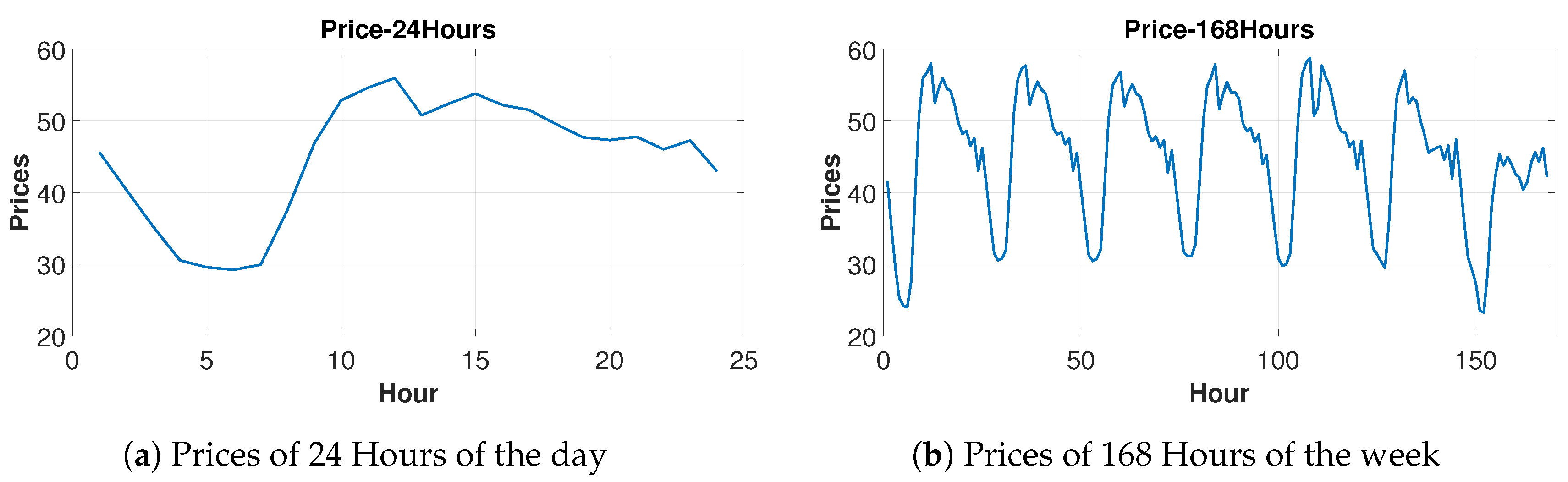
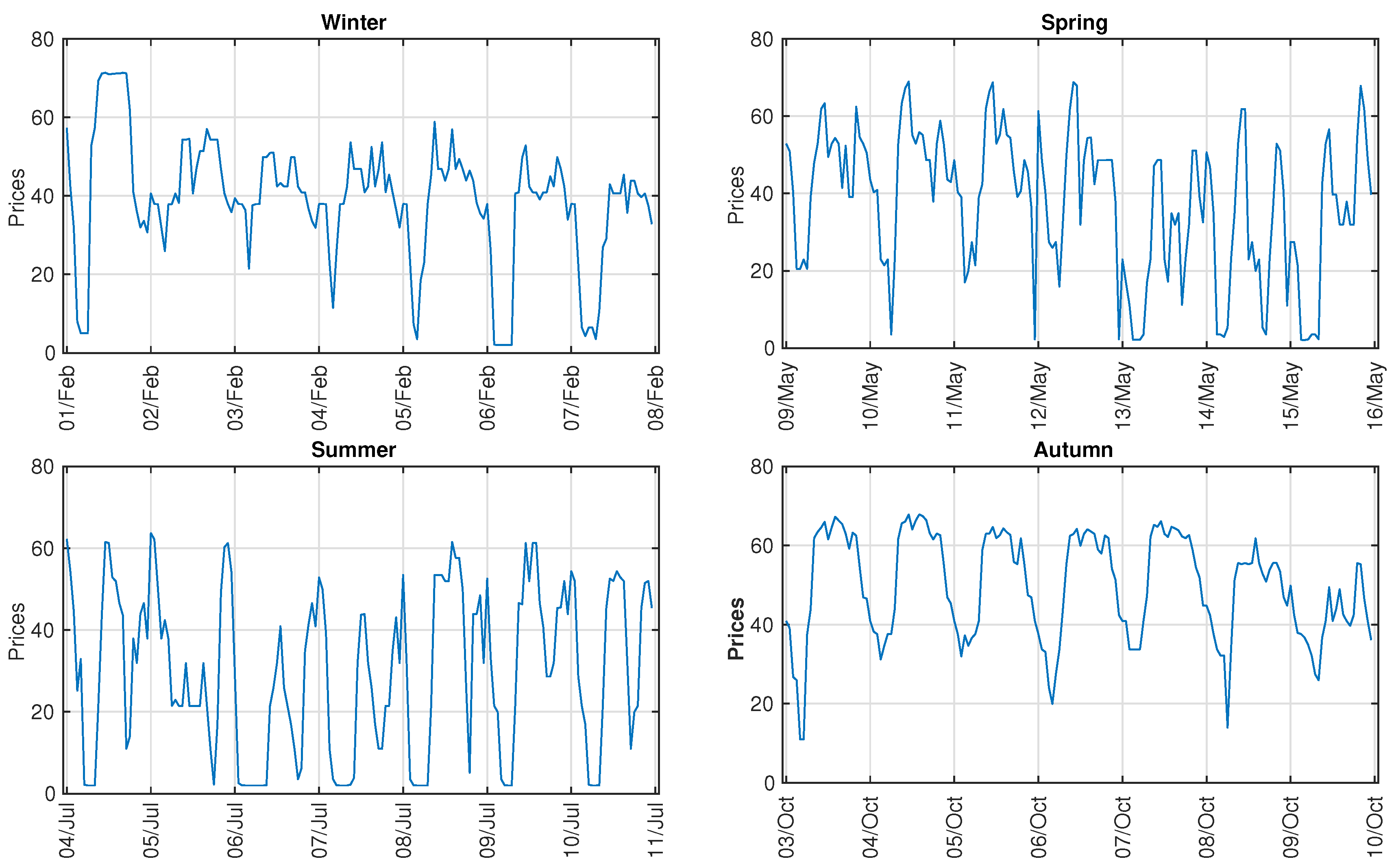
Turkish Day-ahead Market electricity prices are effected by various types of seasonality. Early morning hours (2:00–7:00) have relatively low prices, even some zeros. Moreover, there are double peaks in the day, one before and one after the lunch time, 11:00 and 14:00, respectively, as visualized in Figure 1. In weekly terms, Saturday morning prices are as high as the other weekdays, which shows the working pattern on Saturday mornings. Furthermore, there are two minimums on Saturday night and Sunday night. From a seasonal point of view, both heating and cooling requirements cause high prices in winter and summer, respectively. However, due to the high share of hydro power plants in the electricity production, prices tend to decrease in spring time. An example from the data for each season of 2016 is visualized in Figure 2. The detailed statistics of the test data from 2016 are illustrated in the Appendix A.

Hourly day-ahead electricity prices of the Turkish Day-Ahead Market are obtained from 1 January 2013 to 21 December 2016 [62]. The Turkish Day-Ahead Market was established on 1 December 2011. The first 13 months was excluded due to the learning-by-doing process, which limited us to start our data from 1 January 2013.

In neural network applications, the first three years (1 January 2013–31 December 2015) are used for training and each hour of the next day (1 January 2016) is predicted using the 24-step-ahead forecast scheme. This process is repeated using rolling window method by moving the window 24 h in every forecast. Training period remained as three years and the forecast period as 24-h of the following day. This process is repeated for 356 days of 2016. The reason forf not including the last 10 days of 2016 in the forecast procedure is the very high prices, which occurred in this term due to the natural gas shortage and inactivity of the natural gas power plants. Prices increased up to 515 Euro/MWh on 23 December at 14:00, which is approximately 14 times higher than the average price level.

In the statistical time series methods, such as Markov, Threshold Auto Regressive (TAR) and SARIMA, due to non-stationary nature of the price series and zeros, factorial ANOVA [6] transformation was applied and the series split into deterministic and stochastic parts. Then, stationary stochastic part was forecasted and added to the deterministic part values, which include the hour, weekday, month, holiday and year components. This process was repeated in the rolling window scheme for 356 days as in the neural network methods.

Variable selection is a very important topic in the electricity price forecasting. In our paper, we have chosen the lagged price values as variables according to auto-correlation and partial auto-correlation functions. The chosen lags are also coherent with the lagged price series used in the literature. Furthermore, exogenous variables are also selected according to the electricity price literature [4,31]. Due to the high correlation between them and the independent variable, forecast D/S, temperature and the 24th lags of realized D/S and balancing market price are selected as exogenous variables. One advantage is that the market maker (EPIAS) provides forecast D/S before the bids are given into the system for the next day. Another variable is temperature, which was taken from the Turkish State Meteorological Service as 81 city-based hourly temperatures. Then, annual energy consumption for all the cities was taken from Republic of Turkey Energy Market Regulatory (EPDK) [63] and energy consumption-weighted hourly temperatures (T) were calculated for every hour. Furthermore, we took the 24th lags of realized D/S and balancing market prices into account because both have very high correlation with the price series and also used as variables in the literature. In addition to the above mentioned exogenous variables, 1, 23, 24, 48, 72, 168 and 336 h lagged prices were also utilized as features to estimate the day-ahead prices for the upcoming 24 h. To report the results with aforementioned features, we use the symbols stated in

Table 1. Utilized features for electricity price estimation.

Symbol	Feature
F1	24-h lagged price
F2	168-h lagged price
F3	1-h lagged price
F4	48-h lagged price
F5	23-h lagged price
F6	72-h lagged price
F7	336-h lagged price
F8	Forecast demand over supply
F9	Temperature
F10	Realized demand/supply with 24 h lag
F11	Balancing market price with 24 h lag

.

3. Methods

In this section, we describe the Neural Network architectures we used for electricity price estimation. A simple neural network with three input neurons is visualized in Figure 3. The guiding equation of a neuron can be described as:

$$Y=f(\sum _i^{Inputs}(x_i{w}_i+b_i))$$

where w is the weight on each connection to the neuron, b is the bias and x is the input of the neuron. f can be described as the activation function to introduce non-linearity and, in our experiments, we used Rectified Linear Units (ReLU) [64].

In Section 3.1, basic neural network structure, Artificial Neural Networks, is defined. In Section 3.2, we give a brief definition of Convolutional Neural Networks and their application on the time series data for electricity price estimation. Then, we move to RNNs in Section 3.3, which is the focal point of our work. In Section 3.3.1, we define the LSTM networks and their benefits for time series prediction tasks. Finally, in Section 3.3.2, we define the GRUs and their fundamental differences from LSTMs.

3.1. Artificial Neural Networks

ANN is a basic architecture of a neural network, which consists of layers of neurons connected densely [65]. This type of networks is also known as Multi-layer Perceptrons (MLP) and they are early examples of the neural networks. We used a shallow network with a single layer with 10 neurons and a deeper three-layer network, each consisting of 10 neurons, for our experiments. We added a final layer to estimate the target values.

3.2. Convolutional Neural Networks

Convolutional Neural Networks have been successfully applied to many problems in computer vision [10] and medical image analysis [66]. In our application, the convolutional layers were constructed using one-dimensional kernels that move through the sequence (unlike images where 2D convolutions are used). These kernels act as filters which are being learned during training. As in many CNN architectures, the deeper the layers get, the higher the number of filters become. We used two convolutional layers and a final fully connected layer for prediction. Each convolution is followed by pooling layers to reduce the sequence length.

3.3. Recurrent Neural Networks

RNNs are networks with loops in them, allowing information to persist. They are used to model time-dependent data [67]. The information is fed to the network one by one and the nodes in the network store their state at one time step and use it to inform the next time step. Unlike MLP, RNNs use temporal information of the input data, which make them more appropriate for time series data. An RNN realizes this ability by recurrent connections between the neurons. A general equation for RNN hidden state $h_t$ given an input sequence $x=(x_1,x_2,\dots ,x_T)$ is the following:

$$h_t=\left\{\begin{array}{cc}0,\hfill & \mathrm{if}(t=0)\hfill \\ \varphi (h_{t-1},x_t),\hfill & \mathrm{otherwise}\hfill \end{array}\right.$$

(1)

where $\varphi$ is a non-linear function. The update of recurrent hidden state is realized as:

$$h_t=g(W{x}_t+U{h}_{t-1})$$

(2)

where g is a hyperbolic tangent function.

In general, this generic setting of RNN without memory cells suffers from vanishing gradient problems. In this study, we investigated the performance of two RNNs with memory cells for electricity price forecasting, namely, LSTMs and GRUs.

3.3.1. Long Short-Term Memory Networks

LSTM [68] is a special type of RNN that is able to deal with remembering information for much longer time. In LSTM, each node is used as a memory cell that can store other information in contrast to simple neural networks, where each node is a single activation function. Specifically, LSTMs have their own cell state. Normal RNNs take in their previous hidden state and the current input, and output a new hidden state. An LSTM does the same, except it also takes in its old cell state and outputs its new cell state $c_t^j$ [69]. This property helps LSTMs to address the vanishing gradients problem from the previous time-steps.

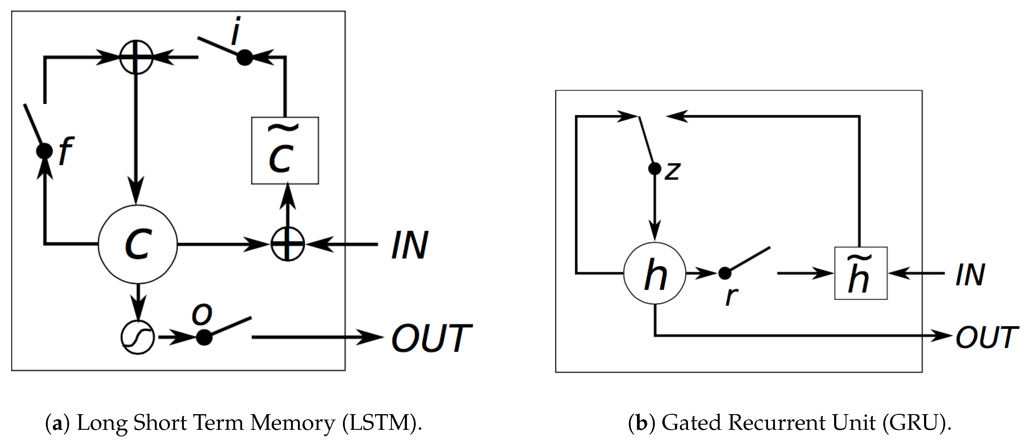
We visualize the LSTM structure in Figure 4a to define the guiding equations of LSTM. LSTM has three gates: input gate $i_t$, forget gate $f_t$ and output gate $o_t$, as visualized in Figure 4a. Sigmoid function is applied to the inputs $s_t$ and the previous hidden state $h_{t-1}$. The goal of the LSTM is to generate the current hidden state at time t. The hidden state $h_t^j$ of LSTM unit is defined as:

$$h_t^j=o_t^j\tan \mathrm{h}(c_t^j)$$

where $o_t^j$ modulates the memory influence on the hidden state. The output gate is computed as:

$$o_t^j=\sigma {(W_o{x}_t+U_o{h}_{t-1}+V_{o}ct)}^j,$$

where $\sigma$ is the logistic sigmoid function and $V_o$ is a diagonal matrix. The memory cell $c_t^j$ is updated partially following the equation

$$c_t^j=f_t^j{c}_{t-1}^j+i_t^j{\tilde{c}}_t^j,$$

where the memory content is defined by a hyperbolic tangent function:

$${\tilde{c}}_t^j=\tan \mathrm{h}{(W_c{x}_t+U_c{h}_{t-1})}^j$$

Forget gate $f_t^j$ controls the amount of old memory loss. Instead, input gate $i_t^j$ controls new memory content that is added to the memory cell. Gates are computed by:

$$f_t^j=\sigma {(W_f{x}_t+U_f{h}_{t-1}+V_f{c}_{t-1})}^j$$

$$i_t^j=\sigma {(W_i{x}_t+U_i{h}_{t-1}+V_i{c}_{t-1})}^j$$

LSTM unit is robust compared to traditional RNN, thanks to the control over the existing memory via the introduced gates. LSTM is can pass information that is captured in early stages and easily keeps memory of this information for long term, which enables the opportunity to generate potential long-distance dependencies as underlined by [70].

3.3.2. Gated Recurrent Units

A GRU [71] has two gates, a reset gate r and an update gate z, as visualized in Figure 4b. The update gate defines how much of the previous memory to be kept and the reset gate determines how to combine the new input with the previous memory. GRUs become equivalent to RNNs, if the reset gates are all 1 and update gates all 0.

Following Chung et al. [70], we formulated the guiding equations. The activation $h_t^j$ of the GRU at time t is a linear interpolation between the previous activation $h_{t-1}^j$ and the candidate activation $h_t^j$:

$$h_t^j=(1-z_t^j)h_{t-1}^j+z_t^j{\tilde{h}}_t^j$$

where an update gate $z_t^j$ is in charge of the content update. The update gate is computed by:

$$z_t^j=\sigma {(W_z{x}_t+U_z{h}_{t-1})}^j$$

This procedure of taking a linear sum between the existing state and the newly computed state is similar to the LSTM unit. Unlike LSTM, GRU does not have any control on the state that is exposed, but exposes the whole state each time.

The candidate activation ${\tilde{h}}_t^j$ is computed similarly to RNN:

$$h_t^j=\tan \mathrm{h}{(W{x}_t+U(r_t\odot h_{t-1}))}^j$$

where $r_t$ is a set of reset gates and ⊙ is an element-wise multiplication.The reset gate $r_t^j$ is computed similarly to the update gate:

$$r_t^j={(W_r{x}_t+U_r{h}_{t-1})}^j$$

GRUs have the same fundamental idea of gating mechanism to learn long-term dependencies compared to LSTM, but there are couple of significant differences. First, GRU has two gates and fewer parameters compared to LSTM. The input and forget gates are coupled by an update gate z and the reset gate r is applied directly to the previous hidden state in GRUs. In other words, the responsibility of the reset gate in an LSTM is divided into both reset gate r and the update gate z. GRUs do not possess any internal memory that is different from the exposed hidden state. LSTMs have output gates and GRUs do not possess output gates. In addition, in LSTMs, there is a second non-linearity applied when computing the output, which is not present in GRUs [72].

4. Results

This section offers a qualitative and quantitative analysis of the proposed method, as well as comparison of RNNs with respect to state-of-the-art methods, to demonstrate its robustness for electricity price estimation.

Our quantitative analysis consists of comparing our method with others and also looking into monthly and weekly performance. In Section 4.1, we describe the evaluation metrics and then explain the state-of-the-art statistical methods in Section 4.2. We report the quantitative results achieved by all network types with a different combination of layers in Section 4.3 and evaluate the statistical significance in Section 4.4. Finally, we mention some implementation details about the neural network training and hyper-parameters in Section 4.5.

4.1. Evaluation Metrics

In the performance evaluation of the forecasting techniques, Mean Absolute Error (MAE), Mean Absolute Percentage Error (MAPE) and Root Mean Square Error (RMSE) are the most used metrics. Although MAPE gives opportunity to compare the electricity price forecasts’ performances from various markets, for the prices around zero, it does not give interpretable results. For zeros, MAPE can not be calculated; for negative prices, there are negative values, which are meaningless; and for small positive prices, MAPE values are very high. In the comparisons, there is not an important difference between the MAE and RMSE values, because both are based on the absolute errors [6]. Therefore, MAE method is used as the performance evaluation criterion in this paper. Equation (3) shows the MAE formula.

$$\mathrm{MAE}=\frac{1}{T}\sum _{i=1}^T\left|P_i-{\widehat{P}}_i\right|$$

(3)

4.2. State-of-the-Art Statistical Methods

Traditionally, Naive method, SARIMA, Markov regime-switching and Self exciting threshold auto-regressive regression (SETAR) have been used with great success for time series estimation in the electricity price forecasting literature [6]. We compared the robustness of these techniques with the neural network architectures.

4.2.1. Naive Method

One of the most important benchmark techniques in the electricity price forecasting literature, naive method [14], can be found below in Equation (4). According to Nogales et al. [14] and Conejo et al. [35], forecasting methods that are poorly calibrated cannot outperform the naive method [6].

$$P_{d,h}=\left\{\begin{array}{cc}{P}_{d-7,h}+{ϵ}_{d,h},\hfill & \mathrm{Monday},\mathrm{Saturday},\mathrm{Sunday}\hfill \\ P_{d-1,h}+{ϵ}_{d,h},\hfill & \mathrm{Tuesday},\mathrm{Wednesday},\mathrm{Thursday},\mathrm{Friday}\hfill \end{array}\right.$$

(4)

$P_{d,h}$ states the price of the selected day and hour. ${ϵ}_{d,h}$ stands for the noise term.

4.2.2. Markov Regime-Switching Auto Regressive (MS-AR) Model

As another benchmark method, two-state Markov regime-switching auto regressive model [73] with the 1st, 24th, 48th and 168th lags of the price series are used in the estimation. This method allows the observations to be distributed into different states by a latent variable. Equation (5) relates the Markov Regime-Switching Auto Regressive (MS-AR) model.

$$y_t=a_s+\sum _{i=1}^p{\varphi }_{s,i}{y}_{t-i}+{ϵ}_t,$$

(5)

where $s_t$ is a two-state discrete Markov-chain with S = 1,2 and ${ϵ}_t\sim i.i.d.N(0,{\sigma }^2)$. The estimation of the MS-AR model is performed by maximum likelihood algorithm [6,74].

4.2.3. Self-Exciting Threshold Auto-Regressive (SETAR) Model

Threshold auto-regressive (TAR) models are similar to Markov regime-switching models in terms of placing the observations into different groups. The main difference of the TAR models is that the threshold variable is observable compared to the latent one in the Markov models. TAR models allow to choose the threshold according to an exogenous variable. If the threshold variable is selected according to a lagged value of the dependent variable, then it is called SETAR model. In Equation (6), SETAR model is given.

$$x_t={\varphi }_0^{\left(j\right)}+{\varphi }_1^{\left(j\right)}{x}_{t-1}+\dots +{\varphi }_p^{\left(j\right)}{x}_{t-p}+{}_t^{\left(j\right)},\mathrm{if}{\gamma }_{j-1}\le x_{t-d}\le {\gamma }_j$$

(6)

where k and d are positive integers; j = 1, …, k; ${\gamma }_i$ are real numbers such that $-\infty ={\gamma }_0<{\gamma }_1<\dots <{\gamma }_{k-1}<{\gamma }_k=\infty$; the superscript (j) is used to signify the regime; and ${\alpha }_t^{\left(j\right)}$ are i.i.d. sequences with mean 0 and variance ${\sigma }_j^2$ and are mutually independent for different j. The parameter d is the delay parameter for different regimes [6,75].

As in Markov model, 1st, 24th, 48th and 168th lags of the price series are used in the estimation, in addition to the delay parameter, d = 1.

4.2.4. Seasonal Auto-Regressive Integrated Moving Average (SARIMA) Model

ARIMA is a special kind of regression, which takes the past prices (AR), previous values of the noise (MA) and the integration level (I) of the price series into account. In SARIMA, seasonal component (S) are also involved in the estimation process. Generally, only intra-weekly nature of the series is incorporated as a seasonal component, but, in the electricity price series, it is required to deal with the intra-daily and intra-yearly seasonality as well. Therefore, triple SARIMA model of [76] is performed by maximum likelihood assuming Gauss–Newton optimization. Equation (7) refers to the triple SARIMA model.

$${\varphi }_p\left(L\right){\Phi }_{p_1}\left({Ł}^{{}_{s_1}}\right){\Omega }_{P_2}\left({Ł}^{{}_{s_2}}\right){\Gamma }_{P_3}\left({Ł}^{{}_{s_3}}\right)(y_t-a-bt)={\theta }_q\left(L\right){\Theta }_{Q_1}\left({Ł}^{{}_{s_1}}\right){\Psi }_{Q_2}\left({Ł}^{{}_{s_2}}\right){\Lambda }_{Q_3}\left({Ł}^{{}_{s_3}}\right){ϵ}_t$$

(7)

$y_t$ is the load in period t, a is a constant term, b is the coefficient of linear deterministic trend term; ${ϵ}_t$ is a white noise error term; Ł is the lag operator; and ${\varphi }_p,{\Phi }_{p_1},{\Omega }_{P_2},{\Gamma }_{P_3},{\theta }_q,{\Theta }_{Q_1},{\Psi }_{Q_2}$ and ${\Lambda }_{Q_3}$ are the polynomial functions of orders $p,p_1,P_2,P_3,q,Q_1,Q_2$ and $Q_3$, respectively [6,76].

Our triple SARIMA model can be stated as ${(1,0,1)}_{1}x{(1,0,1)}_{24}x{(1,0,1)}_{168}$. To comply with the other statistical methods, ARMA(48,48) component is also added to this model.

4.3. Quantitative Analysis

In this section, we report the performance analysis of neural networks in comparison with the state-of-the-art methods. We also use a different combination of features for shallow and deep networks to analyze the prediction accuracy. Finally, we report the monthly average results and illustrate the price estimation accuracy of GRU on a graph.

4.3.1. Comparison with the State of the Art Methods

In our first experimental setup, we use key features of lagged price values 1, 24, 48 and 168 on all described algorithms to compare the one-layered neural network algorithm performance with the state-of-the-art methods. Results in

Table 2. Single-layer day ahead prediction MAE results comparison of neural network based methods with state-of-the-art techniques.

Features	Markov	Naive	SETAR	SARIMA	CNN	ANN	LSTM	GRU
F1–4	8.04	7.95	7.89	7.29	9.82	6.37	5.91	5.71

indicate the neural network models’ success compared to the statistical ones. Recurrent neural networks, LSTM and GRU are the best methods in this comparison. As a note, naive method outperforms two other methods, which is in line with the findings of Contreras et al. [13], Nogales et al. [14] and Conejo et al. [35], mentioning the relatively good performance of naive method.

4.3.2. Shallow Network Comparison

Our first comparison is on shallow network architectures to see the performance of each neural network method. We experiment different network architectures using the many different combinations of features in Table 1 following the findings of the literature.

Table 3. Single-layer day ahead prediction MAE results. Each network of one layer and a final fully connected layer for prediction. CNNs have been implemented two convolutional layers stacked together.

Features	CNN	ANN	LSTM	GRU
F1–2	9.82	8.51	7.79	7.70
F1–4	8.57	6.37	5.91	5.71
F1–7	9.47	6.65	6.01	5.64
F1–8	10.05	8.05	6.22	5.83
F1–9	10.51	9.27	6.16	5.83
F1–10	10.64	9.85	6.02	5.58
F1–11	10.58	9.48	5.93	5.55

demonstrates the addition of new variables into the single-layer neural networks. It should be stated that the addition of 1st and 48th lagged values of the price series to the 24th and 168th lags decrease the MAE values, but addition of the exogenous variables do have a very little or even negative effect.

4.3.3. Deep Network Comparison

To showcase the performance of deeper networks we concatenate three layers for simple ANNs, LSTMs and GRUs. It is evident in

Table 4. Multi-layer day ahead prediction MAE results. Each network of stacked three layers and a final fully connected layer for prediction.

Features	ANN-3	LSTM-3	GRU-3
F1–2	7.63	7.66	5.86
F1–4	5.66	5.66	5.68
F1–7	5.59	5.58	5.57
F1–8	5.84	5.62	5.56
F1–9	6.08	5.70	5.57
F1–10	6.29	5.51	5.41
F1–11	6.20	5.47	5.36

that the GRU still performs the best compared to other techniques. The multiple layer structure comes up with an additional computational cost and, to find the optimal number of layers, we do a test on the algorithms.

In this deep neural networks comparison, CNN is excluded due to the low performance. Addition of the new layers increased the performance in every neural networks mechanism. However, the positive effects of the additional variables are still very small, which is in line with our findings in the shallow network comparison section.

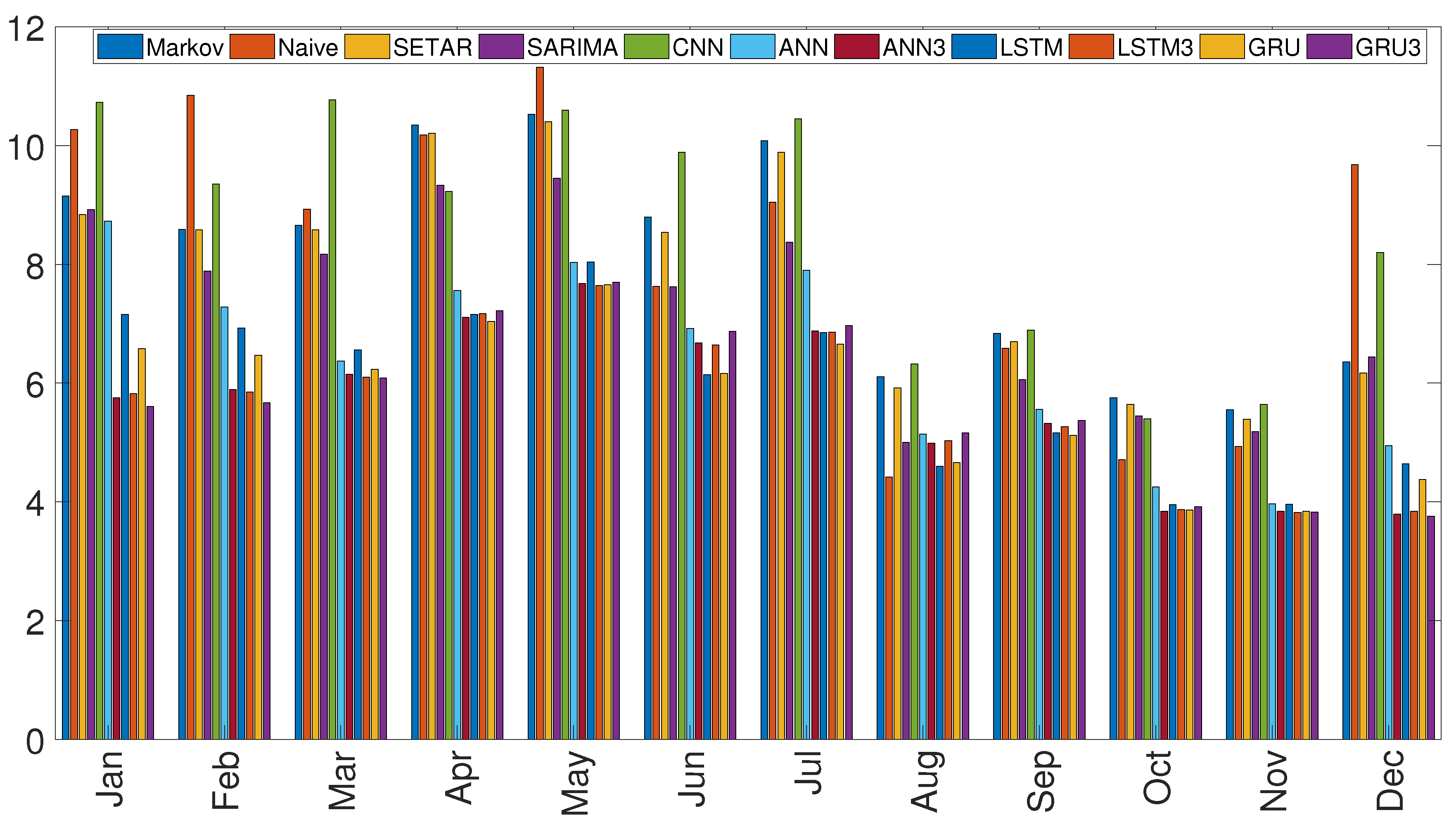
4.3.4. Monthly Comparison

We also evaluated the monthly performance of each technique, as shown in Figure 5. The results for each month are generally consistent with the overall average performance with some exceptional cases. Results demonstrate the relatively good performance of the LSTM and GRU models. Although there are some months that single-layer is better than the multi-layer neural networks, in most of the months, deep neural networks give much better results. With the exception of Naive method in August and three-layer ANN in October, recurrent neural networks, LSTM and GRU, have the best results in every month.

4.3.5. Seasonal Prediction Results

We illustrate the prediction results of GRU for the sample weeks from each season we defined in Section 2. Figure 6 shows the successful performance of GRU with a good match to the original prices. We observe the ability of capturing the spikes, as well as the good performance in relatively calmer periods. It is clear that the performance of the GRU model is great in the relatively calmer autumn week. Moreover, the performance in the summer week, which has a high volatility, gives evidence about the spike detection of the model.

4.4. Diebold–Mariano Tests

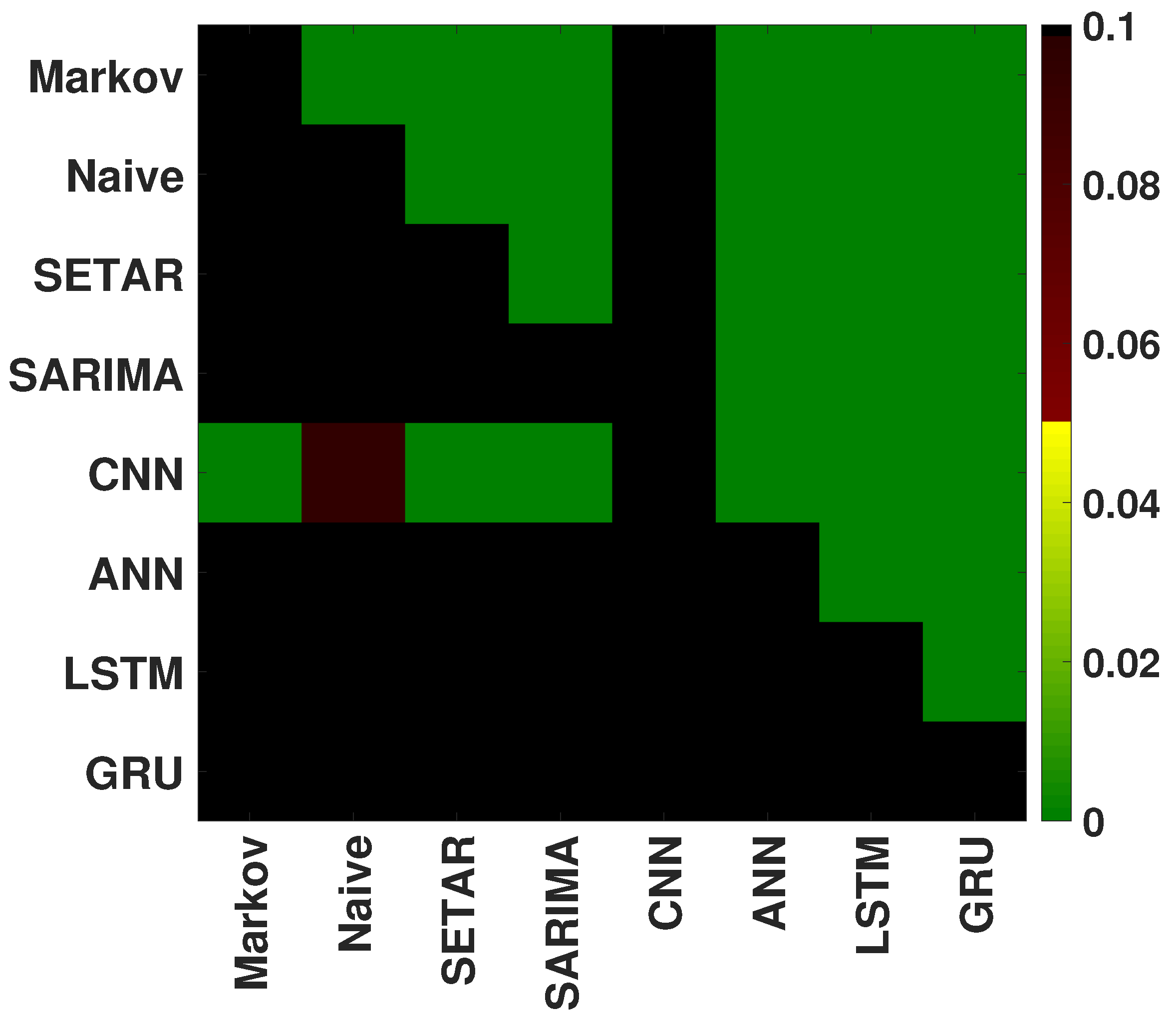
Table 2, Table 3 and Table 4 provide a ranking of the various methods, but not statistically significant conclusions on the performance of the forecasts of one method compared to others. To showcase the statistical significance of the performance difference between all model variations and features combinations, we use a Diebold–Mariano test [61], which takes the correlation structure into account. 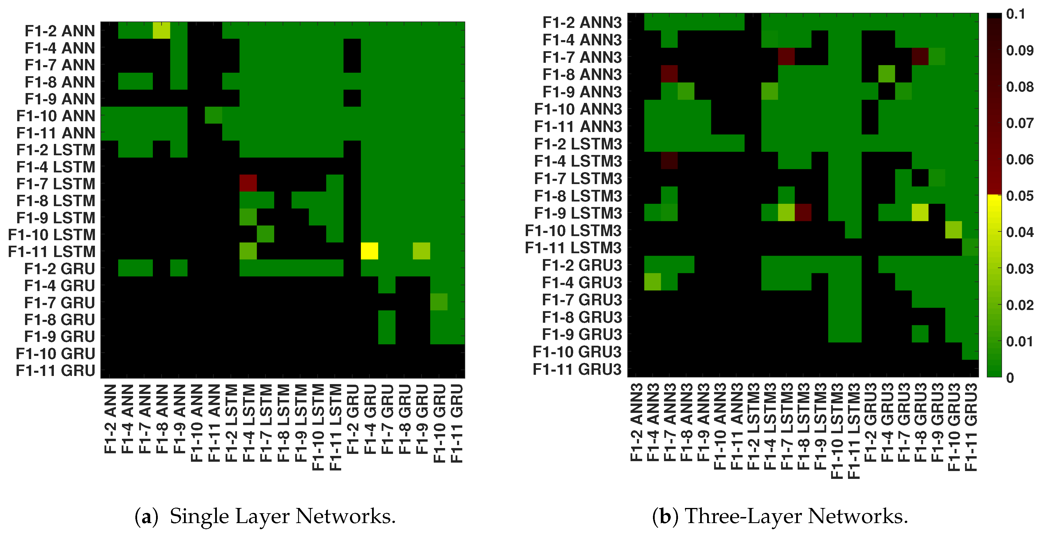In Figure 7, we show the p-values for the Diebold–Mariano tests between neural network based methods and the state-of-the-art statistical methods. In Figure 8, we repeat the same tests for shallow and deep networks using different number of features. It tests the forecasts of each pair of transformations against each other and uses a colour map to show p-values. The low p-values show statistically significant better performance of the methods in X-axis. For example, F1-11 GRU model outperforms all the other models significantly in the three-layer networks comparison (Figure 8b).

Figure 7 demonstrates the successful performance of the neural networks models, except CNN, compared to the statistical methods. Especially, good performance of the recurrent neural network models, GRU and LSTM, is statistically proven by Diebold–Mariano test.

In Figure 8a, single layer networks are compared with each other. F1-10 GRU and F1-11 GRU are significantly better than all the other models. Performance of F1-7 GRU and F1-4 LSTM, which do not include any exogenous variables, should also be mentioned. In Figure 8b, in three-layer networks, addition of new features has a much more significant effect than the single layer network. F1-11 GRU, F1-10 GRU, F1-11 LSTM, and F1-10 LSTM are the best methods among three-layer networks.

4.5. Implementation Details

The training of a neural network can be viewed as a combination of two components, a loss function or training objective, and an optimization algorithm that minimizes this function. In this study, we used the Adam optimizer to minimize the mean absolute error loss function. The training ends when the network does not significantly improve for a predefined number of epochs (300).

During training, a batch-size of three years was used. The momentum of the optimizer was set to 0.90 and the learning rate was 0.001. The parameters of the fully-connected, convolutional, and recurrent layers were initialized randomly from a zero-mean Gaussian distribution. The training continued until no substantial progress was observed in the training loss.

We performed multiple tests to see the performance of different numbers of layers in ANN, LSTM and GRU architectures for selecting the optimal number of layers. Figure 9 shows that the optimal results can be achieved using three layers. Additional layers increase in the total number of parameters and add to the computational cost without achieving a significant gain in the performance.

5. Discussion

In this paper, we investigate the application of various neural network architectures on electricity price forecasting. Our experiments in Table 2 highlight that neural network based methods produce better results compared to the state-of-the-art statistical forecasting methods in the literature such as SARIMA and Markov models. We use simple artificial neural networks (ANNs), CNNs, LSTMs and GRUs to estimate the electricity prices in the Turkish market. We see that the RNN models, namely LSTM and GRU, are able to separate themselves in terms of performance compared to CNNs and simple ANNs in Table 3. This is because RNN models have memory about the previous time steps, which makes them the method of choice for time series type problems. They keep a memory of the previous instances effectively, which is crucial for estimating electricity prices of the day-ahead market.

The deep learning paradigm of stacking multiple layers increases the performance for ANNs, LSTM and GRUs, as highlighted in Table 3 in comparison with Table 4. GRUs still give the best performance among all available techniques and we reached the best results of 5.36 Euros/MWh MAE using three-layered GRUs. The results show good alignment with the prices as illustrated in Figure 6.

Neural networks are data-driven models and their performance heavily depends on the availability of the large training data. The limited data are a deteriorating factor for all training based methods, but in particular for neural network based methods. We show in Figure 9 that the performance does not improve after three layers for any of the networks due to the limited data. With the availability of further data, we believe the overall performance of LSTM and GRU methods will be better.

Another significant observation is the fact that GRUs perform better than the LSTM models. This can explained by the fewer number of parameters that are needed to be learned by GRUs. In the literature, Yin et al. [77] and Chung et al. [70] compared the two models for polyphonic music modelling and speech signal modelling task. They showed the better performance of GRU for these tasks. Moreover, GRUs train faster due to the fact that they require fewer parameters.

We see that the key features are lagged price values for estimating the electricity prices, which is in line with the findings of Uniejewski et al. [4]. In terms of single layer, addition of 1st and 48th lagged values to the 24th and 168th lagged values have an important effect. Especially for LSTM single layer using the 1st, 24th, 48th and 168th lagged values is as good as using all the variables. For GRU, adding 23rd, 72nd and 336th lagged values give better results. Addition of exogenous variables have a very small effect in LSTM. Although addition of forecast D/S and temperature do not have a significant effect in GRU, further addition of 24th lags of realized D/S and balancing market price have significant effects. In three-layer networks, results are similar, but addition of features help much more to have better results. If we do not use any exogenous variables, F1-7 gives better results than F1-4. In three-layer GRU networks, addition of all the variables, except temperature, change the performance significantly. On the other hand, LSTM F1-7 is only worse than LSTM F1-10 and F1-11, which is similar to the single layer results. To conclude, endogenous variables are the most important ones and using the 1st, 24th, 48th and 168th lagged prices give relatively good results. In most cases, adding one or two exogenous variables does not improve the results, but if we use the lagged values of the other exogenous variables, in addition to forecast D/S and temperature, then these models with all the variables significantly outperform the models with fewer variables.

One additional comparison we made was grouping the results in terms of months. It is possible to say that the general error levels are lower in autumn and winter months compared to spring and summer months. In relatively mild weather months of Turkey—October, November and December—three-layer GRU networks’ MAE values are lower than 4 Euros/MWh. On the other hand, relatively hot weather months of Turkey—May, June, and July—have MAE values around 7 Euros/MWh, which is almost double of the mild weather months. It must be mentioned that, in most countries, prices during summer months are not high compared to the other months, but, as mentioned in Section 1.2 on the Turkish market , due to the requirement of air conditioning, prices during summer months are very close to the winter months prices. We can conclude that the MAE values show a similar pattern with the price levels, which demonstrate the effect of the seasonality.

Our results are in line with the main findings of Lago et al. [59], Kuo and Huang [60], which is that machine learning models, especially deep neural networks, outperform the state-of-the-art statistical models and shallow neural networks. On the other hand, in our experiment, deep recurrent neural networks, LSTM and GRU, which are tailor-made for time-dependent problems, give lower errors than DNN, which contradicts with the results of [59]. Lago et al. [59] made two hypotheses about the unexpected superiority of DNN in their paper: first, low amount of data; and, second, different structure of the models. Moreover, they underlined the necessity of further research. In our opinion, having deep LSTM and GRU, instead of shallow LSTM and GRU, causes the conflict between the results. Lago et al. [59] applied single-layer LSTM and GRU, or apply LSTM and GRU as one layer of the hybrid deep neural networks. In our case, there are three layers of LSTM and GRU in the experiments. Another possible explanation is the market specifics. Turkish market has an increasing share of hydro and renewables in the energy production and the market is similar to the Spanish [44] and German [1] markets in some aspects. However, as we know that all the markets have unique characteristics, generalizability to other markets needs further research. Incredibly fast changing nature of the energy markets, especially in the emerging economies, must also be mentioned. Establishment of two nuclear plants in the next five years, inclusion of the solar energy into system in near future and expiration of the subsidies for the wind power plants in two years will change the dynamics of the Turkish market as well. Therefore, further research in Turkish market and in the emerging economies, such as Southeast Europe markets [78] is also required.

Generalization capability of machine learning models is promising for applying our model for different market data. The GRU network architecture can accurately predict the electricity prices in the Turkish market. With the availability of the multiple feature data for each market, the model can be applied to various markets using domain adaptation. However, Aggarwal et al. [79] underlined the superiority of different methods in different markets and combination of multiple methods might be promising in these type of problems. We would like to investigate possibility of using hybrid models to merge benefits of multiple methods. Zhang [80] proposed combining ARIMA and ANN models to forecast the linear and non-linear components of price separately. Chaabanae [81] developed the Zhang [80] method and combined auto-regressive fractionally integrated moving average (ARFIMA) with neural networks model. Guo and Zhao [82] also utilized decomposition, optimization and support vector machine techniques in a hybrid work. In another example, Shrivastava and Panigrahi [83] applied a hybrid wavelet extreme learning machine. Moreover, Alamaniotis et al. [84] combined relevance vector machines and linear regression ensemble optimization. These types of hybrid approaches can aid the performance of RNNs.

The uncertainty of the predictions made by the neural network models can be of great value to assess their utility. Currently Bayesian based neural networks are used to predict the uncertainty of the neural network based predictions [85]. With the developments in machine learning literature, we would like to estimate the uncertainty values of GRUs and LSTMs to increase the reliability of both methods. Recent work by Hwang et al. opens the path for fast and accurate uncertainty estimations of GRUs [86].

One avenue of improvement for our method is to investigate the decomposition techniques. Related to the hybrid models, Neupane et al. [87] proposed an ensemble prediction method by choosing the algorithm and features among a set of them, which give much better forecast results than state-of-the-art techniques. In another work, Hong and Wu [88] applied principal component analysis (PCA) as a dimension reduction method. Ziel [89] and Ludwig et al. [90] used Lasso shrinkage method for variable selection. Zheng et al. [53] proposed using empirical mode decomposition for decomposing the signal to several intrinsic mode functions (IMFs) and residuals. They used these IMFs to train LSTM to forecast short-term load. In the future, we would like to include dimension reduction algorithms and investigate their contribution to seasonality of the data, in particular in RNN setting.

In conclusion, this study instigated the utility of neural networks for electricity price estimation. Development of new conditions in electricity markets across the world brings new challenges. Accurate price estimation is a crucial task for adapting to the new market conditions, and machine learning methods are capable of addressing these issues with high accuracy. Recurrent Neural Networks set the state-of-the-art in addressing time-dependent problems. With this work, we show a detailed analysis on RNNs for electricity price forecasting and highlight the superior performance of GRUs in comparison to various neural network based methods and state-of-the-art statistical techniques.