Nonlinear Robust Control for Low Voltage Direct-Current Residential Microgrids with Constant Power Loads

Abstract

A Direct Current (DC) microgrid is a concept derived from a smart grid integrating DC renewable sources. The DC microgrids have three particularities: (1) integration of different power sources and local loads through a DC link; (2) on-site power source generation; and (3) alternating loads (on-off state). This kind of arrangement achieves high efficiency, reliability and versatility characteristics. The key device in the development of the DC microgrid is the power electronic converter (PEC), since it allows an efficient energy conversion between power sources and loads. However, alternating loads with strictly-controlled PECs can provide negative impedance behavior to the microgrid, acting as constant power loads (CPLs), such that the overall closed-loop system becomes unstable. Traditional CPL compensation techniques rely on a damping increment by the adaptation of the source or load voltage level, adding external circuitry or by using some advanced control technique. However, none of them provide a simple and general solution for the CPL problem when abrupt changes in parameters and/or in alternating loads/sources occur. This paper proposes a mathematical modeling and a robust control for the basic PECs dealing with CPLs in continuous conduction mode. In particular, the case of the low voltage residential DC microgrid with CPLs is taken as a benchmark. The proposed controller can be easily tuned for the desired response even by the non-expert. Basic converters with voltage mode control are taken as a basis to show the feasibility of this analysis, and experimental tests on a 100-W testbed include abrupt parameter changes such as input voltage.

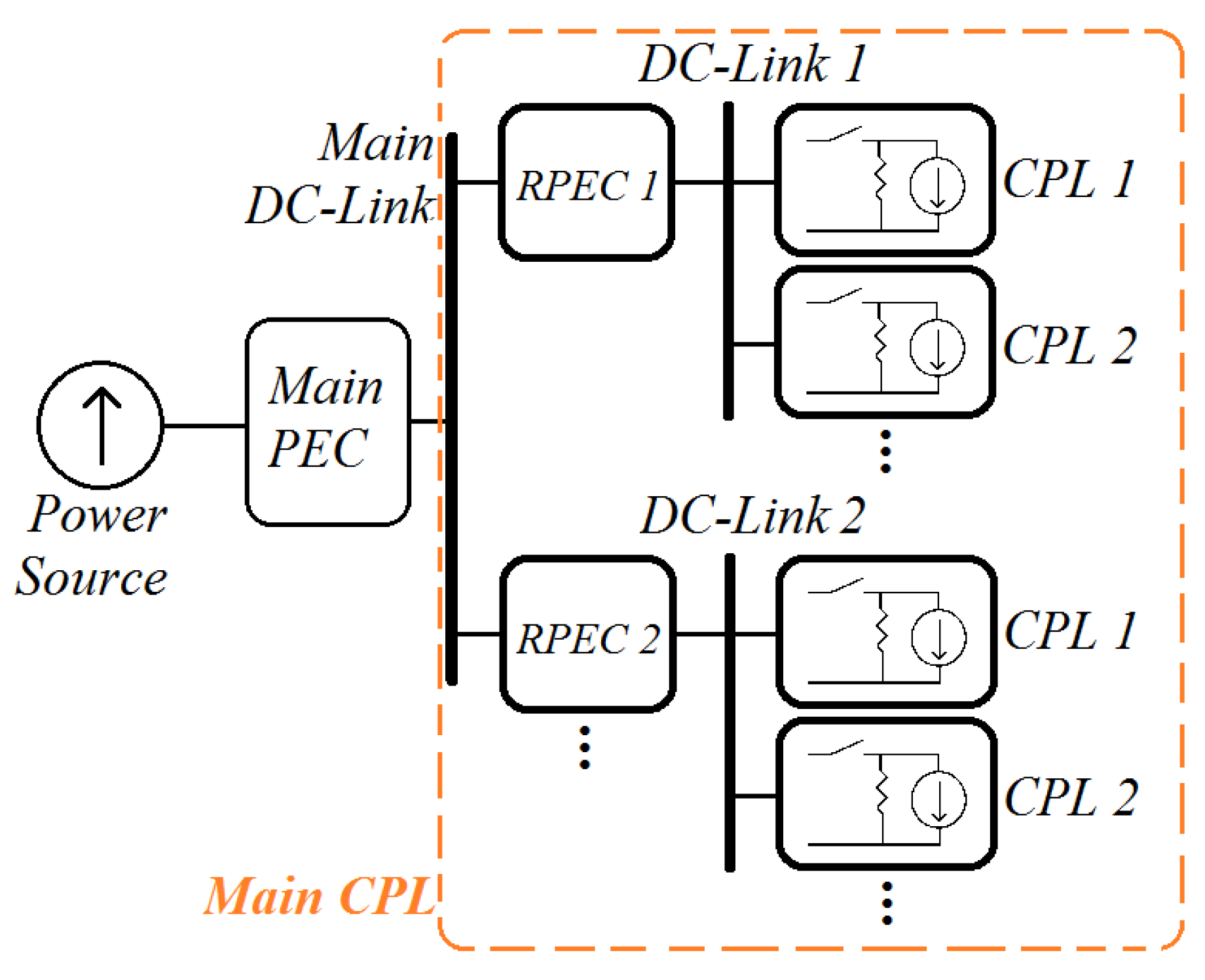
1. Introduction

A Distributed Generation System (DGS) can be understood as a flexible structure in the generation, transmission, distribution and storage of electric energy [1]. Nowadays, it is a common practice to use DGS in smart grids. A smart grid based on a DGS must have the following characteristics: (a) fast response to load transients; (b) energy storage capability, which feeds electricity back to the grid from the client. (c) self-control of power load demands; and (d) intensive use of small power generators based on renewable energy sources [2].

A relatively novel and important kind of smart grid is the DC microgrid. The DC microgrid is generally structured using DC renewable energy sources, for example fuel cells, photovoltaic panels, wind generators with a rectifier and energy storage systems (batteries) with an energy management system, among others. A particularity of the DC microgrid with respect to the smart grids is the integration of different power sources joined through a DC link and connected to local loads. In addition, the energy source can be generated on-site in such a way that the microgrid achieves high efficiency, reliability and versatility [3].

Today, there are numerous electronically-managed power loads that can be connected to the DC-link of a smart grid, such as televisions, electric ovens, coffee makers, LED lamps, computing equipment, among many others. However, it is necessary to mention that power electronics is the key device in the development of a DC microgrid, mainly due to the use of PECs, which allow an efficient power energy conversion between sources and loads. There are different kinds of PECs that can be connected to a DC microgrid in order to reduce, invert or increase the desired/nominal DC-link voltage, i.e., buck, boost, interleaved boost, positive buck/boost, forward, fly-back, half bridge and full bridge converter, to name a few [4].

However, for this paper, a low voltage DC microgrid for building/residential applications similar to the one proposed in [5] is considered as a benchmark. This arrangement is divided into three sections as in the following description. The first one includes high power elements for common building facilities (greater or equal to 538 V and 10 kW), including photovoltaic panels, wind generators, fuel cells, among others. The second one relies on the medium power elements, which are usually found in kitchen appliances and laundry rooms ($[230,400]$ V, $[0.4,10]$ kW). It is necessary to mention that the current loading can remain similar to the 230-V AC system. However, the voltage can be increased up to 400 V if a size reduction is needed. Finally are the low power loads, which include devices located in bedrooms, living rooms and outdoor areas ($[24,48]$ V, less than $0.4$ kW).

It is well known that in a closed-loop scenario, the load can act as a constant power load (CPL) for its source, producing a negative-rate varying resistance (known as negative impedance), which destabilizes the system. Since the theoretical analysis complexity increases with this characteristic, the development of different approaches to ensure the stability of the closed-loop system has been encouraged. Traditional CPL compensation techniques rely on a damping increment by adapting the voltage level of the source or the load, adding external circuits or by using advanced control techniques. An interesting review of these approaches was reported in [6], which classifies the CPLs into two groups, control approaches and auxiliary circuits/power buffer. In the first group, control techniques such as feedback linearization, sliding mode, pulse adjustment and pole placement were reviewed such that their main benefit is that they do not diminish the load performance. In the second group, the instability problem seems solved; however, an auxiliary circuit is needed, increasing the implementation cost and complexity; the overall system stability is omitted.

Another attractive survey can be found in [7] in which a review of the state of the art in the performance and usual properties of DC microgrids connected to CPLs, stability approaches and compensation methods were described. Recently, a novel discrete-time modeling and an active stabilizer for PWM converters was proposed in [8]. This proposal allows performing the stability analysis for the DC distribution systems with nonlinear characteristics. The authors reported that the proposed discrete-time method could identify slow-scale and fast-scale instabilities and also a measure of the sensitivity to some parameter change. The robustness of the proposal to filter the parameters’ variation was also studied. Finally, this proposal was numerically- and experimentally-verified. Nevertheless, a formal analysis of the CPL case is not reported.

On the other hand, an active damping method was stated in [9]. In this paper, a variation of the CPL in the system by attaching a supercapacitor-based energy storage system was proposed. As a result, the CPL’s instability effects can be decreased by virtually increasing the resistive loads. Numerical simulations and practical results were reported. The limitation of this proposal relies on the extra components needed such as a supercapacitor and a bidirectional converter; besides, the production of an energy consumption increase and a slow dynamics response are present.

In contrast, [10] present a sufficient condition for the local stability of DC linear and time-invariant (LTI) circuits with CPLs. A set of steps that should be met for the reported method was also proposed. In order to validate their proposal, two cases were analyzed: a single-port DC RLC circuit with a constant voltage input connected to an ideal CPL and a two-port DC circuit with a single constant voltage input connected to two CPLs, both modeled as LTI systems. Likewise, in [11], a sum of squares (SOS) technique for DC power networks with CPL was presented. In this paper, the region of attraction of the system was estimated by using the SOS and a semidefinite programming algorithm. Additionally, two methods were proposed and compared for the calculation of the region of attraction; it was stated that a reduction of the estimation was achieved by increasing the degree of a Lyapunov function. Furthermore, [12] reported a generalized method to algebraically analyze the stability of DC distribution systems. The authors derive necessary and sufficient conditions for stability by algebraically determining the system’s eigenvalues. Furthermore, an insight into the parameter’s relationship with the DGS stability was presented. Numerical simulations were reported to validate the proposed method, and unfortunately, practical results were not presented. Another interesting approach was reported in [13]. In this paper, a load side compensation technique was proposed by using a sliding mode (SM) approach. Additionally, a comparative study was performed with a PID controller. Besides the good dynamic response achieved by SM, only numerical simulations were reported. In [14], inner and outer control loops for higher order PECs, such as SEPIC, Cuk and Zeta, connected to a CPL were proposed. For the inner loop, a virtual resistance, connected in series with the input inductor, worked as an active damping stage. An integral controller was added in the outer loop with the main aim to compensate the output voltage steady state error. In this paper, the stability conditions for the equilibrium points and a validation given by numerical simulation were reported. Practical experiments for a high order PEC were also reported. In [15], the DC microgrid stability was analyzed for a known quantity of CPLs. In this paper, the problem was formulated as a robust stability problem of a polytopic uncertain linear system and a set of sufficient conditions to guarantee, at least locally, the robust stability. On the other hand, [16] investigated the DC microgrid with a resistive-inductive load in a CPL scheme using a droop control. A stability condition was discussed, and the corresponding stable region was obtained. Validation of the proposal was reported by numerical simulations. Unfortunately, practical results on a test bed were not reported. In [17], two controllers were proposed: the first an integer order and the second a fractional order, for sliding mode controllers in a DC/DC boost converter feeding a CPL on a typical DC microgrid scheme. Nonlinear sliding manifolds and stability were also researched, and numerical simulations to compare their performance were reported. Nevertheless, practical results were not reported. Further information can be found in [18]. Finally, in [19], the DC microgrid stability was analyzed for a known quantity of CPLs. The problem was formulated as a robust stability one for a polytopic uncertain linear system. A set of sufficient conditions to guarantee, at least locally, the robust stability was obtained. Several numerical simulations were reported to show the effectiveness and non-conservativeness of this proposal. Unfortunately, experiments were not performed.

From the previous paragraph, it can be noted that a large amount of research work has been done to solve the instability problem imposed by the CPLs and that many methods have been proposed to overcome the problem, but none of them provide a simple and more general solution for this issue. In this paper, the mathematical modeling, the robust control and the stability analysis for the basic PECs (buck, boost and buck-boost), even in a reconfigurable scheme dealing with CPLs and parameter variation in continuous conduction mode (CCM), are presented to gain knowledge about more complex configurations with CPLs. The reconfigurable converter presented in this paper is a kind of PEC that can change its structure while the activity is going on (on-the-fly), providing a high flexibility and increased operating range with few components; see, for example, [20,21,22].

The major contributions of the proposed approach are listed below:

• Robust stability against arbitrary (bounded) changes in source voltage, output power, inductance and capacitance on the desired operating-point.
• Flexibility for use with the basic converters and even in a reconfigurable scheme.
• Low implementation time and cost.
• Easy tuning for a certain desired response.

This paper is structured as follows. In Section 2, a unified model for the buck, boost and buck-boost PECs, in continuous conduction mode, voltage mode and current mode, is presented; then, the instability with CPLs is analyzed. In Section 3, a feedback linearization is used to build a linear parameter varying (LPV) system of the voltage-mode model. Robust stability against arbitrary (bounded) changes in source voltage and output power are analyzed so that the nonlinear CPL converter is stabilized on the desired operating point. In this section, a discussion is presented regarding the advantages and limitations of this scheme. After that, a Taylor series linearization is introduced for voltage and current mode; the latter in order to obtain the polytopic LPV representation for both cases. The advantages of the polytopic LPV as a natural representation of the CPL converter are highlighted. Subsequently, robust controllers are proposed in order to demonstrate analytically the stability of the polytopic systems despite that the CPLs are alternated/switched. It is necessary to mention that abrupt changes on CPL are a typical condition in renewable energy scenarios. In order to illustrate the robust stability of the proposed controller, even under arbitrary (bounded) changes, a 100-W testbed was implemented by using an inexpensive 100-W P-MOSFET and an 8-bit microchip microcontroller. Representative experimental tests with CPL, while an output voltage stabilization is reached, are presented in Section 4. Tests include parameter changes such as input voltage and CPL alternating. In this section, a brief comparison with other proposals is given. In the last section of this paper, final conclusions are given, which summarize the feasibility of the proposed model and control strategy to be robust in CPL scenarios and to be implemented on a low-cost platform.

2. Modeling

In this section, the models of the unified PEC for voltage-mode control and for current-mode control in continuous conduction mode are presented. That is, the mathematical models that are presented are valid for buck, boost and buck-boost converters. As reported in [7,23], the PEC dynamics for voltage and current control mode in discontinuous conduction mode with CPL are open-loop stable, and they are not within the scope of this article.

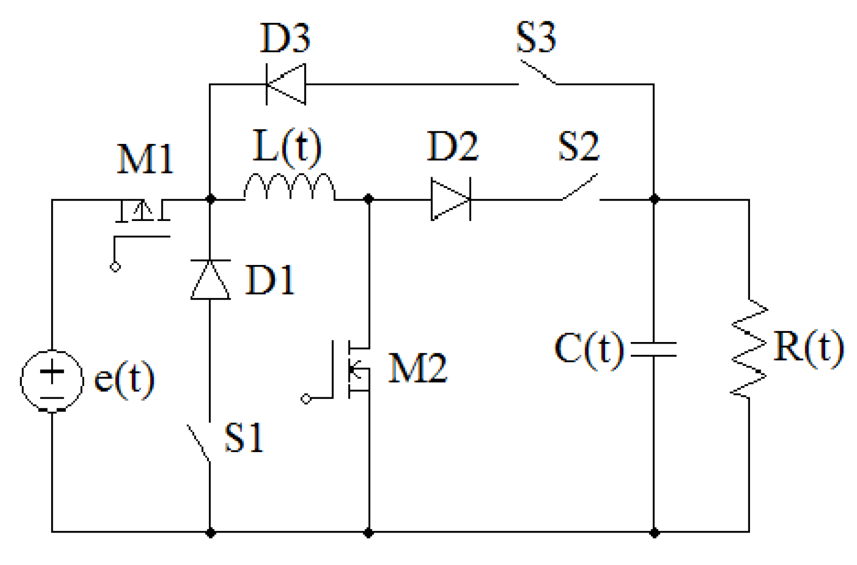
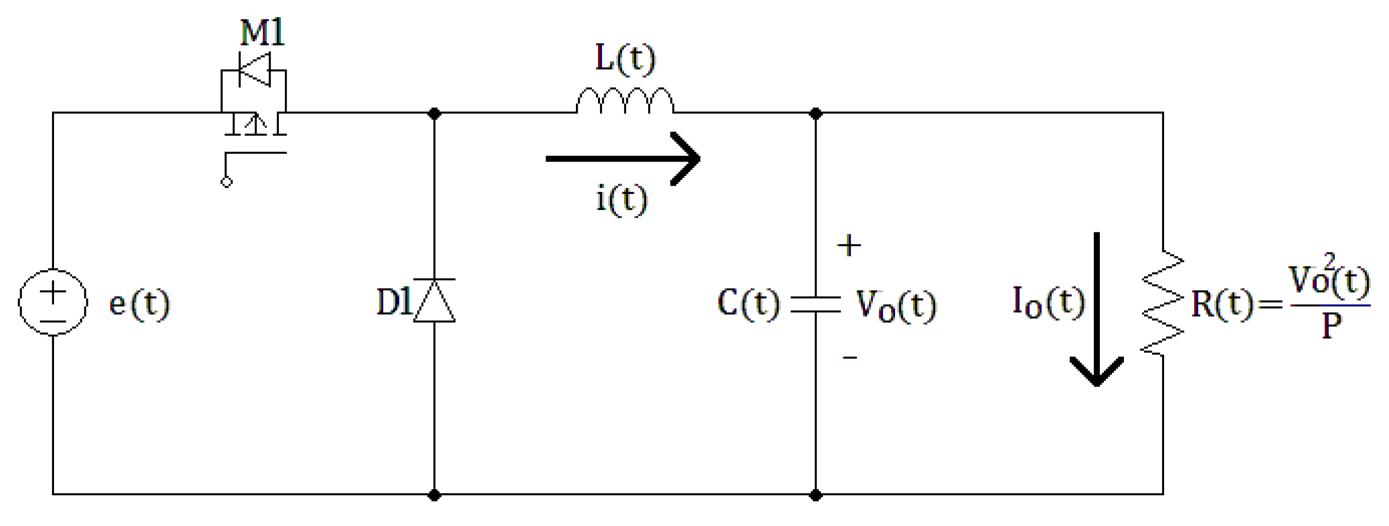
2.1. Voltage-Mode Modeling

In a microgrid scenario, several CPLs are switched depending on client necessities; each load can be modeled as a resistance with an additional current source parallel to its value of current, indirectly proportional to the voltage and directly proportional to the value of the constant power dissipated. A PEC provides adequate voltage/current levels to the CPL, but, since different voltage levels in the DC-link are needed for different kinds of CPLs, a PEC is attached to each DC-link in such a way that a cascaded configuration is structured. An example of such a configuration is shown in Figure 1. For instance, a buck, a boost or a buck-boost converter stands for the PEC in the most common scenarios. In order to consider any of the above PECs, even in an on-the-fly reconfiguration between them, the reconfigurable PEC (RPEC) from [24] is used. This means that the following analysis is valid for any of the mentioned configurations even if a reconfiguration is performed. Consider the RPEC in Figure 2; each mode/reconfiguration can be modeled as follows.

The overall power demand is provided by one or more power supplies; however, this scenario can be easily simplified from the point of view of each RPEC, considering that the power source is a time-varying voltage/current source and that the load is a CPL (orange block in the figure) with a piecewise constant level or even as a fast varying power level. In this study, the CPL is simplified by a time-varying resistance with known bounds (known and bounded CPL levels); for instance, with S1, S2 closed and S3 open, a buck converter is configured with a CPL in its output as shown in Figure 3. In this figure, the schematics of a buck-type PEC with varying parameters are shown. The load resistance $R\left(t\right)$ is indirectly proportional to a constant power value and directly proportional to the square of the output voltage $V_o\left(t\right)$, and it can represent a set of CPLs. Since the objective is to maintain $V_o\left(t\right)$ at a set-point level $V_x$, a voltage/duty cycle representation is obtained as follows.

Consider the nominal values for $E\left(t\right)=e$, $L\left(t\right)=L$ and $C\left(t\right)=C$; note that later in this paper, a design range for the variation of these parameters will be considered for the stability analysis. Similar to [25], by comparing the particular dynamic systems’ descriptions with respect to the MOSFET (M) state, with ideal components, a dynamic model is obtained:

$$\begin{array}{c}\hfill L\frac{di}{dt}=u_{d}e-V_o\end{array}$$

(1)

$$\begin{array}{c}\hfill C\frac{d{V}_o}{dt}=i-\frac{P}{V_o}\end{array}$$

(2)

where the time dependence is omitted for readability and $u_d\in \{0,1\}$ is a discrete function that represents the state of M with a 1 for closed and a 0 for open, in a high enough switching frequency operation. Redefining the control variable $u_d$ as a sufficiently smooth function taking values in the compact interval $\left[0,1\right]$, the averaged dynamic description that predicts the behavior of the PEC with CPL is:

$$\begin{array}{c}\hfill L\frac{di}{dt}=ue-V_o\end{array}$$

(3)

$$\begin{array}{c}\hfill C\frac{d{V}_o}{dt}=i-\frac{P}{V_o}\end{array}$$

(4)

The $C^{\infty }$ differentiability property of the above system allows replacing Equations (3) in (4) to obtain the voltage-mode PEC with the CPL mathematical description:

$$\begin{array}{c}\hfill {\dot{x}}_1=x_2\end{array}$$

(5)

$$\begin{array}{c}\hfill {\dot{x}}_2=\frac{e}{LC}u-\frac{1}{LC}{x}_1+\frac{P}{C{x}_1^2}{x}_2\end{array}$$

(6)

where $x_1=V_o$ and $x_2={\dot{V}}_o$.

From [24], the above mathematical representation is valid also for boost and for buck-boost topologies depending on the u value, that is in a reconfigurable scheme. Three operation modes are allowed, and each one of them is selected by a proper switching activation and by a pulse width modulation (PWM) MOSFET activation:

• S1, S2 closed, S3, M2 open and PWM switching on M1, buck.
• M1, S2 closed, S1, S3 open and PWM switching on M2, boost.
• M2, S3 closed, S1, S2 open and PWM switching on M1, buck-boost.

where the following is obtained:

• a buck PEC if $0\le u\le 1$
• a boost PEC if $u>1$
• a buck-boost PEC if $u<0$

and with the PWM duty cycle for buck ($\check{u}$), boost ($\widehat{u}$) and buck-boost ($\tilde{u}$) calculated by:

• buck duty-cycle for $0\le u\le 1$ is $u=\check{u}$
• boost duty-cycle for $u>1$ is $u=\frac{1}{1-\widehat{u}}$
• buck-boost duty-cycle for $u<0$ is $u=\frac{\tilde{u}}{\tilde{u}-1}$

Note that a few extra components are needed for the reconfigurable on-the-fly topology.

On the other hand, it is known that the instability property of a nonlinear system can be inferred from its linearization instability property (Theorem 4.15 of [26]). The linearization of (5) and (6) in $x_1=V_x$, $x_2=0$ and $u=u_x$ is:

$$\begin{array}{c}\hfill {\dot{x}}_1=x_2\end{array}$$

(7)

$$\begin{array}{c}\hfill {\dot{x}}_2=\frac{e}{LC}u-\frac{1}{LC}{x}_1+\frac{P}{C{V}_x^2}{x}_2\end{array}$$

(8)

and it has the following transfer function:

$$\frac{x_2\left(s\right)}{u\left(s\right)}=\frac{e}{LC{s}^2-\frac{PL}{V_x^2}s+1}$$

(9)

whose poles remain in the right-side complex semi-plane, even with no varying parameters, so that the instability property can be extended to the nonlinear system. Therefore, technically there exists the possibility of an output voltage drop for the open loop PEC with CPL even with time-invariant parameters. In the following section, a nonlinear control law that stabilizes the (7) and (8) system, even with varying parameters, is shown.

2.2. Current-Mode Modeling

From the dynamic system (1) and (2), it is easy to demonstrate that:

$$\begin{array}{c}\hfill \frac{d{I}_o}{dt}=\frac{I_o^3-i{I}_o}{CP}\end{array}$$

(10)

$$\begin{array}{c}\hfill \frac{di}{dt}=\frac{ue}{L}-\frac{P}{I_{o}L}\end{array}$$

(11)

with u defined as in the previous section. The $C^{\infty }$ differentiability property of the above system allows replacing Equations (10) in (11) to obtain the unified mathematical description:

$$\begin{array}{c}\hfill {\dot{y}}_1=y_2\end{array}$$

(12)

$$\begin{array}{c}\hfill {\dot{y}}_2=\frac{2y_1^2{y}_2}{CP}+\frac{y_2^2}{y_1}-\frac{eu{y}_1}{CPL}+\frac{1}{LC}\end{array}$$

(13)

where $y_1=I_o$ and $y_2={\dot{I}}_o$. The linearization of (12) and (13) in $y_1=I_r$, $y_2=0$ and $u=u_y$ is:

$$\begin{array}{c}\hfill {\dot{y}}_1=y_2\end{array}$$

(14)

$$\begin{array}{c}\hfill {\dot{y}}_2=-\frac{e{I}_r}{CPL}u-\frac{e{u}_y}{CPL}{y}_1+\frac{2I_r^2}{CP}{y}_2+\frac{1}{LC}+\frac{e{u}_y{I}_r}{CPL}\end{array}$$

(15)

and it has the following transfer function:

$$\frac{y_2\left(s\right)}{u\left(s\right)}=\frac{I_y}{CPL{s}^2-2L{I}_y^{2}s+u_y}$$

(16)

whose poles remain in the right-side complex semi-plane, in a way that the instability property can be extended to the nonlinear system.

3. Controller Design and Stability

In the following, linearization is used in order to determine a linear parameter varying system for a robust stability analysis. Firstly, a feedback linearization is performed in voltage mode, and after, Taylor series linearizations are performed for voltage and current mode control. Once each linear system is obtained, a simplice polytopic system is constructed that allows a stability analysis by means of a common Lyapunov function, as well as appropriate values of the controllers’ gains. Note that the controllers are easy to implement for linearizations in Taylor series.

3.1. Feedback Linearization for Voltage-Mode Controller

Consider the system (5) and (6). A feedback linearization is performed in order to obtain a linear polytopic system, with the main aim to demonstrate that it is robust against arbitrary parameter changes. The feedback proposed is as follows:

$$u=-k_1{x}_1-\left(\frac{PL}{e{x}_1^2}+k_2\right)x_2$$

(17)

where $k_1,k_2$ are controller gains; the system under the above controller action is obtained substituting u in the system (5) and (6):

$$\begin{array}{c}\hfill {\dot{x}}_1=x_2\end{array}$$

(18)

$$\begin{array}{c}\hfill {\dot{x}}_2=-{\alpha }_1{x}_1-{\alpha }_2{x}_2\end{array}$$

(19)

where:

$$\begin{array}{c}\hfill {\alpha }_1=\frac{k_{1}e+1}{LC}\end{array}$$

(20)

$$\begin{array}{c}\hfill {\alpha }_2=\frac{k_{2}e}{LC}\end{array}$$

(21)

Selecting $k_1>0$ and $k_2>0$, one has that ${\alpha }_1>0$ and ${\alpha }_2>0$.

Consider parametric variation within known ranges, denoted by an underline for the minimum value and by an overline for the maximum value, as follows: $e\left(t\right)\in \left[\underline{e},\overline{e}\right]$, $L\left(t\right)\in \left[\underline{L},\overline{L}\right]$ and $C\left(t\right)\in \left[\underline{C},\overline{C}\right]$. The linearized system (18) and (19) can be written as a polytopic, simplice system [27]:

$$\begin{array}{c}\hfill \dot{x}={\theta }_1{A}_{1}x+{\theta }_2{A}_{2}x+{\theta }_3{A}_{3}x+{\theta }_4{A}_{4}x\end{array}$$

(22)

where $\mathsf{\Theta }={\theta }_1+{\theta }_2+{\theta }_3+{\theta }_4=1$, ${\theta }_1\ge 0, {\theta }_2\ge 0, {\theta }_3\ge 0, {\theta }_4\ge 0$ (simplice) and:

$$A_1=\left[\begin{array}{cc}0& 1\\ -{\underline{\alpha }}_1& -{\underline{\alpha }}_2\end{array}\right],A_2=\left[\begin{array}{cc}0& 1\\ -{\underline{\alpha }}_1& -{\overline{\alpha }}_2\end{array}\right],A_3=\left[\begin{array}{cc}0& 1\\ -{\overline{\alpha }}_1& -{\underline{\alpha }}_2\end{array}\right],\mathrm{and}{A}_4=\left[\begin{array}{cc}0& 1\\ -{\overline{\alpha }}_1& -{\overline{\alpha }}_2\end{array}\right].$$

(23)

That is, ${\underline{\alpha }}_1$ is the minimum value of ${\alpha }_1$ for the defined parametric variation ranges and similarly for the other bound of ${\alpha }_1$ and the boundaries of ${\alpha }_2$. From [28], the quadratic stability of the system (22) is ensured if it is quadratically stable with ${\theta }_1=1$, with ${\theta }_2=1$, with ${\theta }_3=1$ and with ${\theta }_4=1$:

Proposition 1.

[28] The quadratic stability of the system (22) is equivalent to the existence of a $P\in {\mathbb{R}}^{2\times 2}$ symmetric, positive definite matrix satisfying:

$$P{A}_i+A_i^{T}P\prec 0,\forall i=1,\dots ,4$$

(24)

where $A_i$ denotes the i-th vertex and $·\prec 0$ denotes a definite negative matrix.

That is, it is enough to demonstrate quadratic stability for all vertices; in fact, in such a case, a common Lyapunov function (CLF) can be constructed from one of the vertices. With that objective, from [26], every eigenvalue of the $A_i$-th matrix must take a negative real value in order to determine the quadratic stability of the vertex; it can be resolved that the second vertex conditions are the supreme, and it is enough to accomplish (see Appendix A for a proof):

$$\begin{array}{c}\hfill k_1>\frac{\overline{LC}}{4\underline{e}}{\left(\frac{k_2\overline{e}}{\underline{LC}}\right)}^2-\frac{1}{\underline{e}}\end{array}$$

(25)

$$\begin{array}{c}\hfill k_2>0\end{array}$$

(26)

to ensure the robust quadratic stability; so, it can be concluded that the proposed feedback linearization (17) stabilizes the nonlinear system (5) and (6) if the gains $k_1,k_2$ are selected so that (25) and (26) are met.

3.2. Taylor Series Linearization for Voltage-Mode Controller

Although a direct feedback linearization can be carried out in order to nullify the nonlinear term in (6), as described in the previous section, possibly time-varying and hardly-estimable terms are involved, for example $L\left(t\right)$. Instead of a direct feedback linearization, consider the Taylor-series linearization (7) and (8) and consider once again known ranges for parameter variation, additionally with $V_x\left(t\right)\in \left[{\underline{V}}_x,{\overline{V}}_x\right]$ as the output voltage operating point range, $P\left(t\right)\in \left[\underline{P},\overline{P}\right]$ as the output power range and the linear feedback $u=-k_3{x}_1-k_4{x}_2$. A polytopic, simplice system can be constructed as in Section 3.1, [27]:

$$\begin{array}{c}\hfill \dot{x}={\theta }_1{\mathcal{A}}_{1}x+{\theta }_2{\mathcal{A}}_{2}x+{\theta }_3{\mathcal{A}}_{3}x+{\theta }_4{\mathcal{A}}_{4}x\end{array}$$

(27)

where:

$${\mathcal{A}}_1=\left[\begin{array}{cc}0& 1\\ -{\underline{\sigma }}_1& -{\underline{\sigma }}_2\end{array}\right],{\mathcal{A}}_2=\left[\begin{array}{cc}0& 1\\ -{\underline{\sigma }}_1& -{\overline{\sigma }}_2\end{array}\right],{\mathcal{A}}_3=\left[\begin{array}{cc}0& 1\\ -{\overline{\sigma }}_1& -{\underline{\sigma }}_2\end{array}\right],\mathrm{and}{\mathcal{A}}_4=\left[\begin{array}{cc}0& 1\\ -{\overline{\sigma }}_1& -{\overline{\sigma }}_2\end{array}\right],$$

(28)

Following the same technique used in Section 3.1, it is easy to demonstrate that:

$$\begin{array}{c}\hfill {\sigma }_1=\frac{e{k}_3+1}{LC}\end{array}$$

(29)

$$\begin{array}{c}\hfill {\sigma }_2=\frac{k_{4}e}{LC}-\frac{P}{C{V}_x^2}\end{array}$$

(30)

where the $\sigma$ boundaries are constructed with the boundaries of the parameter variation ranges as in the previous section. The stability of all of the vertices is ensured if:

$$\begin{array}{c}\hfill k_3>0\end{array}$$

(31)

$$\begin{array}{c}\hfill 0<\frac{k_4\underline{e}}{\overline{LC}}-\frac{\overline{P}}{\underline{C}{\underline{V_x}}^2}<2\sqrt{\underline{{\sigma }_1}}\end{array}$$

(32)

It is worth mentioning that in this analysis, there is no restriction on the rate of change in the parameters including the value of the constant power transferred to the load. Therefore, it can be concluded that the proposed feedback, stabilizes the polytopic system (27) if the gains $k_3,k_4$ are selected so that (31) and (32) are met. In order to accomplish these conditions, first select a $k_3$ and calculate ${\sigma }_1$ to determine the maximum value of $k_4$.

Note that several linearizations in different operating points can be performed to obtain a switched polytopic system, and the global stability can be demonstrated by a CLF; however, it is not the objective of this paper. Refer to [29] for a switched polytopic stability approach.

3.3. Taylor Series Linearization for Current-Mode Controller

In current-mode, a feedback linearization as in the case of voltage-mode is not possible due to the squared current change ($y_2^2$). In this case, a direct linearization of (12) and (13) in the operating point $y_1=I_r$, $y_2=0$, $u=u_y$ and variable changes $z_1=y_1-I_r$, $z_2=y_2$ are performed:

$$\begin{array}{c}\hfill {\dot{z}}_1=z_2\end{array}$$

(33)

$$\begin{array}{c}\hfill {\dot{z}}_2=\frac{e{u}_y}{CPL}{z}_1+\frac{2I_r^2}{CP}{z}_2-\frac{e{I}_r}{CPL}u\end{array}$$

(34)

Consider $u=k_5{z}_1+k_6{z}_2$ where $k_3,k_4>0$ are controller gains; the system (33) and (34) is now:

$$\begin{array}{c}\hfill {\dot{z}}_1=z_2\end{array}$$

(35)

$$\begin{array}{c}\hfill {\dot{z}}_2=-{\gamma }_1{z}_1-{\gamma }_2{z}_2\end{array}$$

(36)

where:

$$\begin{array}{c}\hfill {\gamma }_1=\frac{k_{5}e{I}_r}{CPL}-\frac{e{u}_y}{CPL}\end{array}$$

(37)

$$\begin{array}{c}\hfill {\gamma }_2=\frac{k_{6}e{I}_r}{CPL}-\frac{2I_r^2}{CP}\end{array}$$

(38)

Again, a polytopic system can be built as follows:

$$\begin{array}{c}\hfill \dot{z}={\vartheta }_1{\mathcal{A}}_{1}z+{\vartheta }_2{\mathcal{A}}_{2}z+{\vartheta }_3{\mathcal{A}}_{3}z+{\vartheta }_4{\mathcal{A}}_{4}z\end{array}$$

(39)

where:

$${\mathcal{A}}_1=\left[\begin{array}{cc}0& 1\\ -{\underline{\gamma }}_1& -{\underline{\gamma }}_2\end{array}\right],{\mathcal{A}}_2=\left[\begin{array}{cc}0& 1\\ -{\underline{\gamma }}_1& -{\overline{\gamma }}_2\end{array}\right],{\mathcal{A}}_3=\left[\begin{array}{cc}0& 1\\ -{\overline{\gamma }}_1& -{\underline{\gamma }}_2\end{array}\right],\mathrm{and}{\mathcal{A}}_4=\left[\begin{array}{cc}0& 1\\ -{\overline{\gamma }}_1& -{\overline{\gamma }}_2\end{array}\right].$$

(40)

For the quadratic stability of the system (39), every eigenvalue of the ${\mathcal{A}}_i$-th matrix must take a negative real value in order to determine the quadratic stability of the vertex. Calculating such conditions for ${\gamma }_1,{\gamma }_2>0$, for all $A_i$ and for all the eigenvalues results in the controller gains conditions:

$$\begin{array}{c}\hfill k_5>\frac{\overline{P}\overline{L}\overline{C}}{\underline{e}{\underline{I}}_r}\left[\frac{1}{4}{\left(\frac{k_6\overline{e}{\overline{I}}_r}{\underline{P}\underline{L}\underline{C}}-\frac{2{\overline{I}}_r^2}{\overline{P}\overline{C}}\right)}^2+\frac{\overline{e}{\overline{u}}_y}{\underline{P}\underline{L}\underline{C}}\right]\end{array}$$

(41)

$$\begin{array}{c}\hfill k_6>\frac{2{\overline{I}}_r^2\overline{P}\overline{L}\overline{C}}{\underline{e}{\underline{I}}_r\underline{C}\underline{P}}\end{array}$$

(42)

It is worth mentioning that, in this analysis, there is no restriction about the rate of change in the parameters including the value of the constant power transferred to the load. Once again, it can be concluded that the proposed feedback stabilizes the polytopic system (39) if the gains $k_5,k_6$ are selected in a way that (41) and (42) are met.

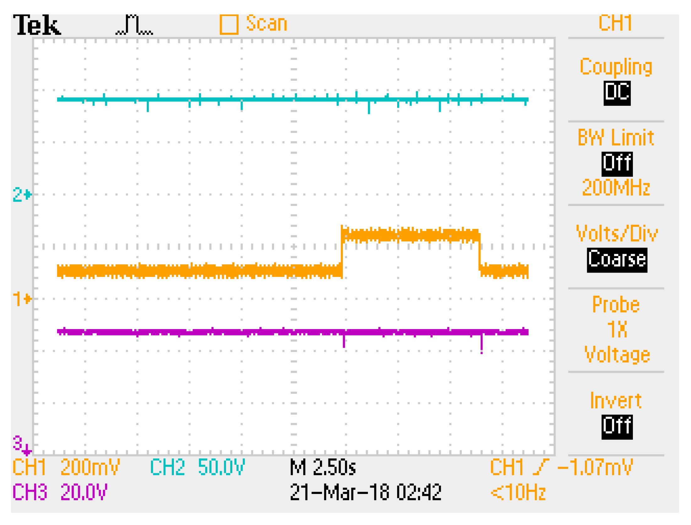
4. Experimental Behavior

In order to illustrate the robust stability of the proposed controller even under arbitrary (bounded) changes, a 100-W testbed was implemented (Figure 4) for a buck topology (although simulations were performed for a wide variety of tests including at high power ranges, such data are not presented here; the interested reader can refer to the Data Availability Section at the end of the paper for PSIM 11 schematics and data). At the top is a low voltage power source that feeds the low control board voltage at the bottom. In the middle are the power source and the electronic load from top to bottom.

The buck topology was selected due to lowering of the voltage, which is the most required case for the LVDCdistribution system for building/residential applications. Indeed, it is required to decrease the voltage from the main 375-V DC bus in the following cases: (a) loads with input rectifier (325 V DC); (b) loads with pure resistive loads (230 V DC); (c) loads without protection against indirect contacts (120 V DC); (d) light electronic appliance loads, based on the standard telecommunication industry (48 V DC); (e) EMerge Alliance Occupied Space Standard loads (24 V DC); and (f) automotive loads (12 V DC).

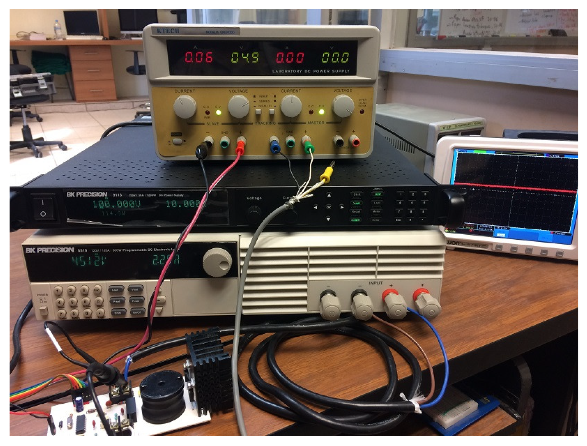
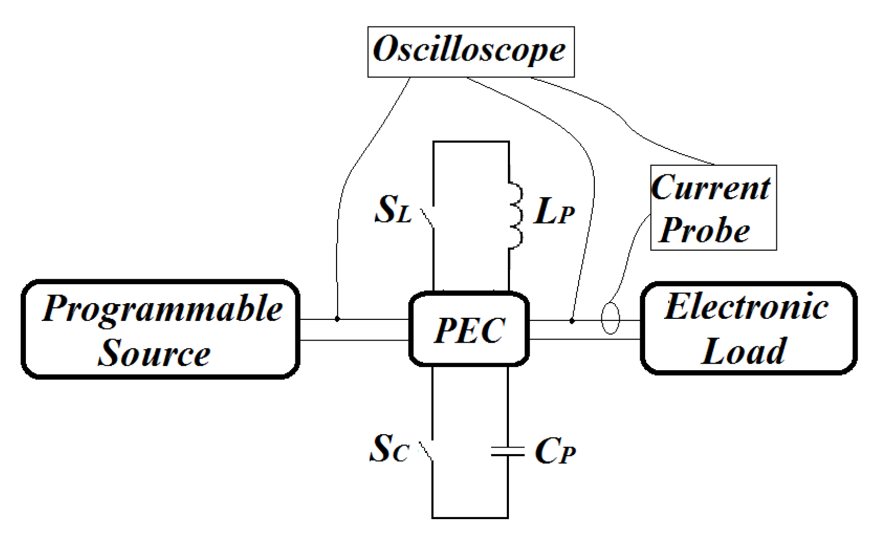
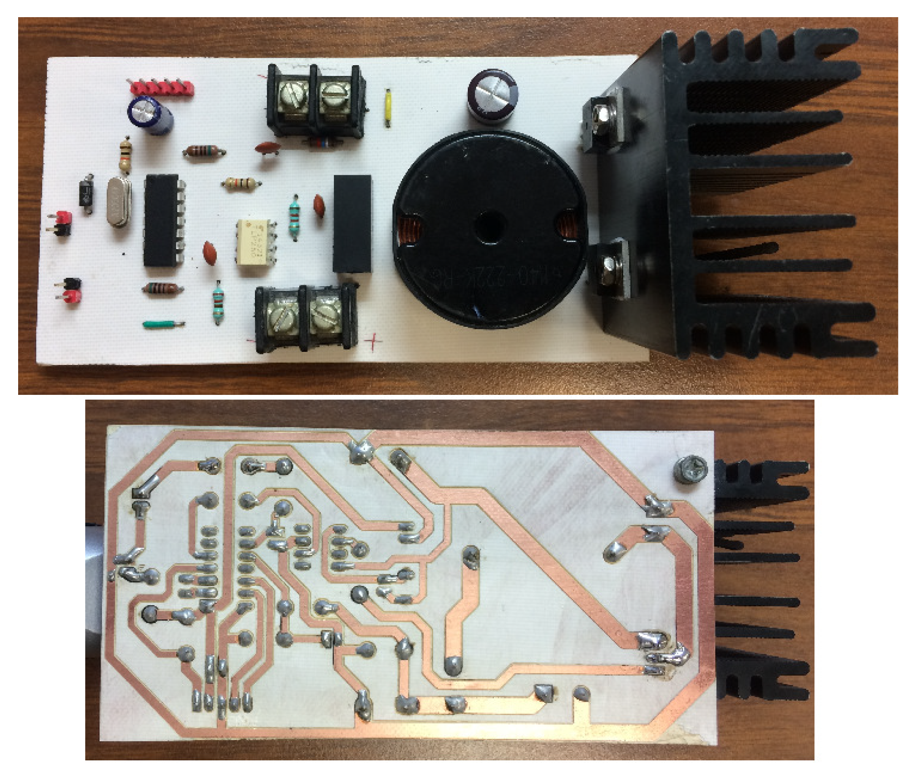
4.1. Equipment

In Figure 5, the configuration of the testbed used to perform the demonstrative experiments is shown. The PEC and PWM were built in a single PCB. The PCB that was built is shown in Figure 6. The low cost of the PEC, the 8-bit Microchip microcontroller running at 20 MHz, sampling at 625 kHz and the common 120-W P-MOSFET that were used, is worth highlighting. A programmable medium power DC power source (1200 W), Model 9116 from BK PRECISION, was used for the input; this source allows obtaining abrupt changes in output voltage and current. Additionally, a 600-W programmable DC electronic load, Model 8510 from BK PRECISION, was used as the output; this device allows setting a constant power (CPL) for some desired voltage or current and performs abrupt changes in the power level on-the-fly. Two mechanical switches $SL$ and $SC$ were laid to perform abrupt changes of the passive components of the PEC; that is, to connect/disconnect a parallel capacitor/inductor ($CP$/$LP$) with C and L. The output current is measured with a Tektronix A622 current probe with 100 mV/A (1 A) connected to a four-channel oscilloscope; the input and output voltages are measured by a direct connection to the oscilloscope.

The parameter boundaries for this testbed were as follows: $L\in \left[2.2\mathrm{mH},2.4\mathrm{mH}\right]$, $C\in \left[0.9\mathsf{\mu }\mathrm{F},1.1\mathsf{\mu }\mathrm{F}\right],P\in \left[45\mathrm{W},100\mathrm{W}\right],e\in \left[80\mathrm{V},100\mathrm{V}\right]$. The voltage-mode robust controller (Section 3.2) was selected for the experiments due to its implementational simplicity (no current measure is performed to calculate the control output), such that controller gains that fulfill (31) and (32) were tuned with $V_x=48$ V. That is, first, $k_3=3.5>0$ was tuned to obtain a desired behavior, and with this value, ${\sigma }_1$ was calculated to determine the value of $k_4$ that fulfills (32); in such a case, $k_4$ results in a very low positive value.

4.2. Procedure

In order to show the validity of the analysis of this paper, several tests were performed in the testbed described in the previous section. The overall tests were performed at normal temperature conditions (22 degrees for the room temperature and 40 degrees at the heat sink).

The first representative test consists of performing abrupt input voltage changes emulating a real microgrid scenario. For a 100-W CPL the following sequence of input voltage changes was used: $90\mathrm{V}$, $80\mathrm{V}$, $70\mathrm{V}$, $80\mathrm{V}$, $90\mathrm{V}$ and $100\mathrm{V}$. The output voltage response is shown in Figure 7 in purple at the bottom, while the input voltage is shown in blue at the top and the output current in yellow in the middle. The CPL is maintained at 50 W at 48 V.

The second representative test consisted of CPL changes, that is the constant power load value was modified in the following sequence: $50\mathrm{W}$, $1\mathrm{W}$, $80\mathrm{W}$ and $1\mathrm{W}$, in order to recreate a scenario with several CPLs in a changing ON-OFF condition with $e=80\mathrm{V}$. No adverse effects were detected in this test, as shown in Figure 8; again, the output voltage response is shown in purple at the bottom, while the input voltage is shown in blue at the top and the output current in yellow in the middle.

The third representative test consisted of performing a capacitance abrupt change by connecting a series capacitor of $3.9$ $\mathsf{\mu }\mathrm{F}$ with C through a switch (mechanical). The first 5 s (approximately) shown in Figure 9 correspond to a 1 $\mathsf{\mu }\mathrm{F}$ capacitance; then, the switch is turned on up to 10 sto increase the capacitance to $4.9$ $\mathsf{\mu }\mathrm{F}$, which is out of the design bounds. Note that the current ripple in the CPL increases slightly since more current is needed to charge the capacitor; however, the CPL voltage remains stable without transients. This procedure is repeated one time, as shown in the figure.

The fourth test consisted of performing an inductor abrupt change by a switch (mechanical). A parallel inductor of the same nominal value ($2.3$ mH) is connected to L from zero to 5 s (approximately) till the total inductance is $1.15$ mH, which is out of the design bounds. Then, the switch is turned off, and the inductance turns to $2.3$ mH up to 10 s. Note that in spite of a CPL current ripple increase (with a small inductance), the CPL voltage remains stable without transients. This procedure is repeated as shown in the Figure 10.

The last representative test presented in this paper was performed demanding a power load wattage from 50 W to 110 W, which is out of the design boundary $[45,100]$ W; Figure 11 shows the obtained results; note that the controller was able to maintain the output voltage without signals of instability, and only a small voltage transient of a $15\%$ was perceived during the CPL change.

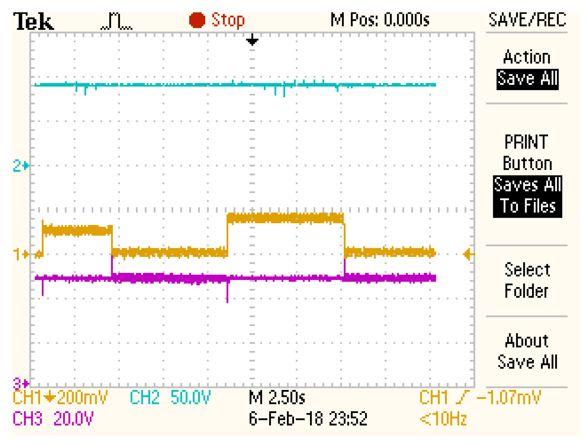
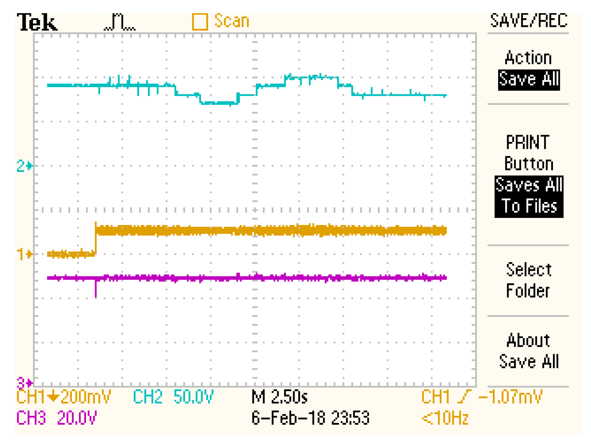
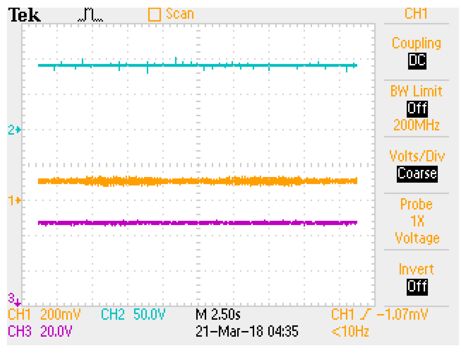
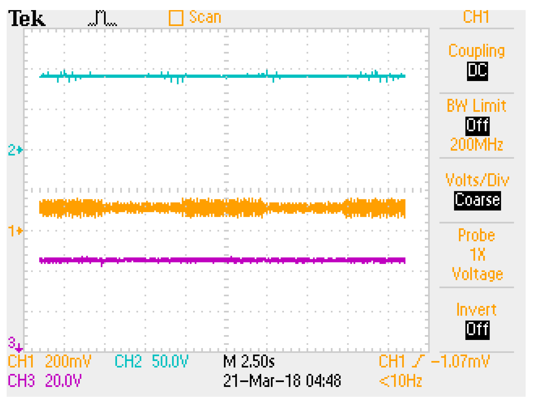
4.3. Discussion of the Results

For the first test, Figure 7 shows the results obtained for both the input and CPL voltage, as well as the CPL current, during abrupt input voltage changes. This is a normal situation in an LVDC microgrid since the voltage is provided from a non-regulated source. In spite of the abrupt changes in input voltage, it is easily seen that the CPL holds with a constant output voltage as expected from the analysis. Note that a small output transient is presented at the beginning of the test; this is reasonable since a derivative controller was used, and initially, the absolute value of the error is high. This can be diminished (if desired) by an ad hoc tuning.

One difficulty encountered during the experiment was that an abrupt increment in the CPL value can easily damage the MOSFET if the voltage is low because the current increases rapidly. The solution was to use a MOSFET, with an adequate working voltage ($V_{DS}=200$ V).

For the second test, Figure 8 shows the results obtained for abrupt CPL changes. In this test, another LVDC microgrid real scenario is emulated since some loads in the microgrid can connect/disconnect from the bus unexpectedly. In spite of abrupt changes in CPL, it is easily seen that the CPL holds with a stable output voltage as expected from the analysis. Note that the CPL voltage ripple increases slightly when the CPL level is low (this is external to the boundaries of the design $[45,100]$ W).

For the third test, Figure 9 shows the results obtained for abrupt capacitance (C) changes. In this test, another real LVDC microgrid scenario is emulated since some loads in the microgrid can provide a parasitic impedance and/or the temperature or another variable can change the total capacitance of the PEC/RPEC. In spite of abrupt changes in capacitance, it is easily seen that the CPL holds with a stable output voltage as expected from the analysis. Note that the CPL voltage ripple increases slightly when the capacitance is high (as in the previous test; this is external to the boundaries of the design $[0.9,1.1]$ $\mathsf{\mu }\mathrm{F}$).

For the fourth test, Figure 10 shows the results obtained for abrupt inductance (L) changes. As in the previous test, another real LVDC microgrid scenario is emulated for parasitic impedances. In spite of the abrupt changes, it is easily seen that the CPL holds with a stable output voltage as expected from the analysis. Note that the CPL current ripple increases when the inductance is low (again, this is external to the boundaries of the design $[2.2,2.4]$ mH).

Finally, the fifth test emulates a CPL that is external to the boundaries of the design with a maximum of 110 W. Note in Figure 11 that a small output transient is present at every change due to the derivative action, but in spite of those, the CPL voltage remains stable.

4.4. Brief Comparison with Other Proposals

Though this proposed controller has an easy operation and dynamic response, its advantages have to be corroborated by comparing it with other proposals. In this paper, not only its complexity, theory and implementation, but also, the dynamic response is evaluated in order to fulfill this purpose. Because no experimental setup was built for additional proposals, the evaluation is performed based on data from existing literature on the subject. A brief comparison for the proposed controller with other schemes is given in

Table 1. Comparison with other proposals.

Type of Controller	Theory Difficulty	Implementation Complexity	Dynamic Response	Remarks
Active stabilizer [8]	High	High	Good	Good performance and a digital platform is used, in this case, a dSPACE.
Active damping [9]	Medium	Medium	Good	Good performance and a digital platform is used, in this case a pair of DSPs.
Linear [10]	High	High	Good	Good performance and only numerical results are reported.
Sum of squares [11]	High	High	Medium	Medium performance and only numerical results are reported.
Algebraic [12]	Medium	Medium	Medium	Medium performance and only numerical results are reported.
Sliding mode [13]	Medium	High	Good	Good performance and only numerical results are reported.
Linear damping [14]	Medium	High	Good	Good performance and a digital platform is used, in this case a DSP.
Robust stability [15]	High	High	Medium	Medium performance and only numerical results are reported.
Drop control [16]	High	High	Good	Good performance and only numerical results are reported.
Fractional order controller [17]	High	High	Medium	Medium performance and only numerical results are reported.
Robust stability [19]	High	High	Medium	Medium performance and only numerical results are reported.
Proposed approach	Medium	Low	High	Good performance and a low cost digital platform is used, in this case, a microcontroller.

. These are found to be classified in terms of the theory and implementational difficulty.

It may be observed that the proposed approach presents a good compromise between theory implementation and dynamic response. Although most of the controllers that are based on non-linear models propose comparable characteristics, the active damping presents a good dynamic response [8]. However, it requires a more sophisticated digital platform for its implementation. Additionally, as seen in Table 1, several controllers are validated with only numerical simulations [10,11,12,13,15,16,17,19]. In contrast, this proposed controller offers a good dynamic response in comparison with the previous work. Additionally, as reported in Table 1, this proposal has a similar response to active damping; however, it does not require much time to cope with CPL, since no sophisticated digital platform is required.

Without a doubt, this proposal requires a natural digital implementation, however not necessarily a sophisticated one (an 8-bit microcontroller is used for the experimental tests). Besides, there are mathematical and experimental conditions where the controller may be operated properly, which do not occur with other proposals. For instance, abrupt changes in passive parameters. Although an in-depth practical comparison may be performed between references [8,9,14] and this proposal, this is beyond the purposes of this publication.

5. Conclusions

In the present work, the CPL stabilization problem was analyzed from a robust-polytopic point of view, for three basic converters even in a reconfigurable scheme while the activity is going on (on-the-fly).

It was also demonstrated that the design of a polytopic, robust controller is natural for the CPL problem since the ranges of power demand and other parameters are normally known. This controller is robust against reasonable (design) changes in the power source voltage/current level and in the values of the components.

It was analytically demonstrated and experimentally shown that a simple controller is enough to stabilize a CPL voltage/current even when all of the parameters are time-varying values if some conditions are met. Various scenarios of LVDC were emulated, and the validity of the analysis presented can be easily extended to other topologies of PEC, even for those reconfigurable ones while the activity is going on (on-the-fly).

The presented controller can be used in various real microgrid scenarios in which a stabilization of the output voltage with parameters that change with time and a piecewise constant power demand are present. The proposed controller and DC-DC converter can be extended for use in electric vehicles.

References

- Wang, P.; Goel, L.; Liu, X.; Choo, F.H. Harmonizing AC and DC: A hybrid AC/DC future grid solution. IEEE Power Energy Mag. 2013, 11, 76–83. [Google Scholar] [CrossRef]
- Kakigano, H.; Nomura, M.; Ise, T. Loss evaluation of DC distribution for residential houses compared with AC system. In Proceedings of the International Power Electronics Conference (IPEC), Sapporo, Japan, 21–24 June 2010; pp. 480–486. [Google Scholar]
- Wang, B.; Sechilariu, M.; Locment, F. Intelligent DC microgrid with smart grid communications: Control strategy consideration and design. IEEE Trans. Smart Grid 2012, 3, 2148–2156. [Google Scholar] [CrossRef]
- Hart, D.W. Power Electronics; Tata McGraw-Hill Education: New York, NY, USA, 2011. [Google Scholar]
- Rodriguez-Diaz, E.; Chen, F.; Vasquez, J.C.; Guerrero, J.M.; Burgos, R.; Boroyevich, D. Voltage-level selection of future two-level LVdc distribution grids: A compromise between grid compatibiliy, safety, and efficiency. IEEE Electr. Mag. 2016, 4, 20–28. [Google Scholar] [CrossRef]
- AL-Nussairi, M.K.; Bayindir, R.; Padmanaban, S.; Mihet-Popa, L.; Siano, P. Constant power loads (cpl) with microgrids: Problem definition, stability analysis and compensation techniques. Energies 2017, 10, 1656. [Google Scholar] [CrossRef]
- Singh, S.; Gautam, A.R.; Fulwani, D. Constant power loads and their effects in DC distributed power systems: A review. Renew. Sustain. Energy Rev. 2017, 72, 407–421. [Google Scholar] [CrossRef]
- Zadeh, M.K.; Gavagsaz-Ghoachani, R.; Martin, J.P.; Nahid-Mobarakeh, B.; Pierfederici, S.; Molinas, M. Discrete-time modeling, stability analysis, and active stabilization of dc distribution systems with multiple constant power loads. IEEE Trans. Ind. Appl. 2016, 52, 4888–4898. [Google Scholar] [CrossRef]
- Chang, X.; Li, Y.; Li, X.; Chen, X. An active damping method based on a supercapacitor energy storage system to overcome the destabilizing effect of instantaneous constant power loads in dc microgrids. IEEE Trans. Energy Convers. 2017, 32, 36–47. [Google Scholar] [CrossRef]
- Arocas-Pérez, J.; Griño, R. A local stability condition for dc grids with constant power loads. IFAC-PapersOnLine 2017, 50, 7–12. [Google Scholar] [CrossRef]
- Herrera, L.; Yao, X. Computation of stability metrics in DC power systems using sum of squares programming. In Proceedings of the IEEE 18th Workshop on Control and Modeling for Power Electronics (COMPEL), Stanford, CA, USA, 9–12 July 2017; pp. 1–5. [Google Scholar]
- Van der Blij, N.H.; Ramirez-Elizondo, L.M.; Spaan, M.T.; Bauer, P. Stability of DC Distribution Systems: An Algebraic Derivation. Energies 2017, 10, 1412. [Google Scholar] [CrossRef]
- Hossain, E.; Perez, R.; Padmanaban, S.; Siano, P. Investigation on the development of a sliding mode controller for constant power loads in microgrids. Energies 2017, 10, 1086. [Google Scholar] [CrossRef]
- Srinivasan, M.; Kwasinski, A. European Conference on Power Electronics and Applications. In Proceedings of the International Power Electronics Conference (IPEC), Warsaw, Poland, 11–14 Sptember 2017; pp. 1–10. [Google Scholar]
- Garces, A. Uniqueness of the power flow solutions in low voltage direct current grids. Electr. Power Syst. Res. 2017, 151, 149–153. [Google Scholar]
- Zhao, Z.; Hu, J.; Xue, H.; Huang, R.; Li, X.; Zhang, X. Large signal stability analysis of DC microgrid under droop control with constant power load. In Proceedings of the Chinese Automation Congress, Jinan, China, 20–22 October 2017; pp. 1046–1051. [Google Scholar]
- Asghar, M.; Khattak, A.; Rafiq, M.M. Comparison of integer and fractional order robust controllers for DC/DC converter feeding constant power load in a DC microgrid. Sustain. Energy Grids Netw. 2017, 12, 1–9. [Google Scholar]
- Chen, Y.; Petras, I.; Xue, D. Fractional order control-a tutorial. In Proceedings of the American Control Conference (ACC’09), St. Louis, MO, USA, 10–12 June 2009; pp. 1397–1411. [Google Scholar]
- Liu, J.; Zhang, W.; Rizzoni, G. Robust stability analysis of dc microgrids with constant power loads. IEEE Trans. Power Syst. 2018, 33, 851–860. [Google Scholar] [CrossRef]
- Momayyezan, M.; Hredzak, B.; Agelidis, V.G. A Load-Sharing Strategy for the State of Charge Balancing Between the Battery Modules of Integrated Reconfigurable Converter. IEEE Trans. Power Electron. 2017, 32, 4056–4063. [Google Scholar] [CrossRef]
- Momayyezan, M.; Hredzak, B.; Agelidis, V.G. Integrated Reconfigurable Converter Topology for High-Voltage Battery Systems. IEEE Trans. Power Electron. 2016, 31, 1968–1979. [Google Scholar] [CrossRef]
- Rizzo, R.; Spina, I.; Tricoli, P. A single input dual buck-boost output reconfigurable converter for distributed generation. In Proceedings of the International Conference on Clean Electrical Power (ICCEP), Taormina, Italy, 16–18 June 2015; pp. 767–774. [Google Scholar]
- Grigore, V.; Hatonen, J.; Kyyra, J.; Suntio, T. Dynamics of a buck converter with a constant power load. In Proceedings of the 29th Annual IEEE Power Electronics Specialists Conference, (PESC’98), Fukuoka, Japan, 22–22 May 1998; Volume 1, pp. 72–78. [Google Scholar]
- Licea, M.A.R.; Pinal, F.J.P.; Gutiérrez, A.I.B.; Ramírez, C.A.H.; Perez, J.C.N. A Reconfigurable buck, boost, and buck-boost Converter: Unified Model and Robust Controller. Math. Prob. Eng. 2018, 2018, 6251787. [Google Scholar] [CrossRef]
- Sira-Ramirez, H.J.; Silva-Ortigoza, R. Control Design Techniques in Power Electronics Devices; Springer Science & Business Media: Berlin, Germany, 2006. [Google Scholar]
- Khalil, H. Nonlinear Systems; Prentice Hall: Upper Saddle River, NJ, USA, 2002. [Google Scholar]
- Lay, S.R. Convex sets and their applications. In Pure and Applied Mathematics; John Wiley and Sons: Hoboken, NJ, USA, 1982. [Google Scholar]
- Boyd, S.; El Ghaoui, L.; Feron, E.; Balakrishnan, V. Linear Matrix Inequalities in System and Control Theory; SIAM: Philadelphia, PA, USA, 1994. [Google Scholar]
- Licea, M.R.; Cervantes, I. Robust indirect-defined envelope control for rollover and lateral skid prevention. Control Eng. Pract. 2017, 61, 149–162. [Google Scholar] [CrossRef]