Power Transformer Operating State Prediction Method Based on an LSTM Network

Abstract

The state of transformer equipment is usually manifested through a variety of information. The characteristic information will change with different types of equipment defects/faults, location, severity, and other factors. For transformer operating state prediction and fault warning, the key influencing factors of the transformer panorama information are analyzed. The degree of relative deterioration is used to characterize the deterioration of the transformer state. The membership relationship between the relative deterioration degree of each indicator and the transformer state is obtained through fuzzy processing. Through the long short-term memory (LSTM) network, the evolution of the transformer status is extracted, and a data-driven state prediction model is constructed to realize preliminary warning of a potential fault of the equipment. Through the LSTM network, the quantitative index and qualitative index are organically combined in order to perceive the corresponding relationship between the characteristic parameters and the operating state of the transformer. The results of different time-scale prediction cases show that the proposed method can effectively predict the operation status of power transformers and accurately reflect their status.

1. Introduction

Power transformers suffer from the long-term effects of high-voltage electric, thermal, and mechanical stresses during operation [1]. In the event of a fault, not only is the transformer seriously damaged, but people’s normal life and production are greatly threatened. Predicting the state of a transformer would help to recognize a potential threat in time and grasp the development trend of the fault. State prediction provides more opportunities to handle potential faults in advance and greatly reduce negative impacts on the transformer’s reliability and availability when a fault occurs [2,3].

Assessment and prediction technologies to determine the health condition of power transformers have been reported in the following aspects. Some studies have focused on predicting specific state parameters, such as gas concentration dissolved in the oil [2,3], top oil temperature [4], residual flux [5,6], inrush current [7], moisture in the insulating cellulose [8], and furan [9], to characterize the development of the transformer’s status. A small number of studies have put forward new ideas for establishing a transformer failure rate model [10,11]. In addition, some scholars have paid special attention to the remaining life [12,13,14,15] of the transformer. The state prediction models proposed in these studies include the neural network [4], support vector machine regression [2,3], fuzzy logic [14], nonparametric regression [10], and probabilistic graph [16]. These methods have demonstrated their effectiveness in a number of circumstances, and some research results have been obtained.

The transformer often deteriorates gradually, rather than abruptly. Correspondingly, the related parameters change continuously towards the status of fault. Thus, it is natural to employ temporal analysis methods to model the sequential dependency between the state parameters over time. Recurrent neural networks (RNNs) [17] have been proven as an effective tool to model temporal dependency in various applications. Xu et al. [18] introduced a novel method based on the RNN to assess the health status of hard drives via the sequence of their attributes. Experimental results show that the RNN method can effectively evaluate the health status of the hard drives and play the role of fault prediction. Tian and Zuo [19] developed an extended recurrent neural network (ERNN)-based approach for predicting the health condition of gearboxes based on the vibration data collected from an experimental gearbox system. The long short-term memory (LSTM) network [20] [21], as an improved structure of the RNN, to some extent, relieved the problem of gradient dissipation and explosion in the modeling process of RNN over a long time, which gained the academic attention of the research community. An LSTM approach for the estimation of remaining useful life was proposed by Zheng et al. [22]. This method can make full use of the sensor sequence information and expose hidden patterns within the sensor data with multiple operating conditions, faults, and degradation models. Kong et al. [23] proposed an LSTM RNN-based framework to tackle the issue of short-term load forecasting for individual electric customers.

The existing assessment/prediction methods are mainly based on a single or a few state parameters to make the analyses and judgments. The status assessment results are always far from comprehensive and cannot reflect the objective rules between the fault evolution and state characteristics [24]. With the improvement of information technology and network technology, relevant application systems such as on-line monitoring systems, production management systems (PMS), dispatching automation systems, and meteorological information systems can realize data sharing and interaction. It is thus urgent to conduct information fusion processing and analysis on all kinds of data to tap the characteristic information that represents the operating state of a transformer.

The accumulation of the transformer state panoramic information provides the prerequisite for the evaluation and prediction of the transformer operating state. In this paper, we use the transformer-condition-related data to employ analysis of transformer status evolution via a deep learning method. A data-driven equipment state correlation analysis and state prediction model is built to realize the preliminary warnings of potential failures of the equipment. This can help identify the equipment that needs specific attention. Based on the key parameters of the operating state, this paper proposes a method for predicting the running conditions of power transformers based on the LSTM network. By combining the quantitative and qualitative indicators, the LSTM prediction model explores the relationship between the characteristic parameters and the transformer state. The feasibility and accuracy of this method are verified through case studies.

The rest of the paper is organized as follows: Section 2 introduces the basic information on the long short-term memory recurrent neural networks. Section 3 provides further information on the proposed transformer operating state prediction approach. Section 4 validates the prediction approach with different case studies and discusses the obtained results. Finally, conclusions are presented in Section 5.

2. Long Short-Term Memory Recurrent Neural Networks

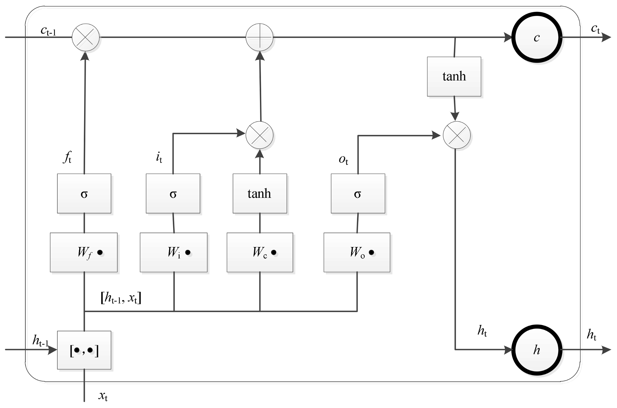
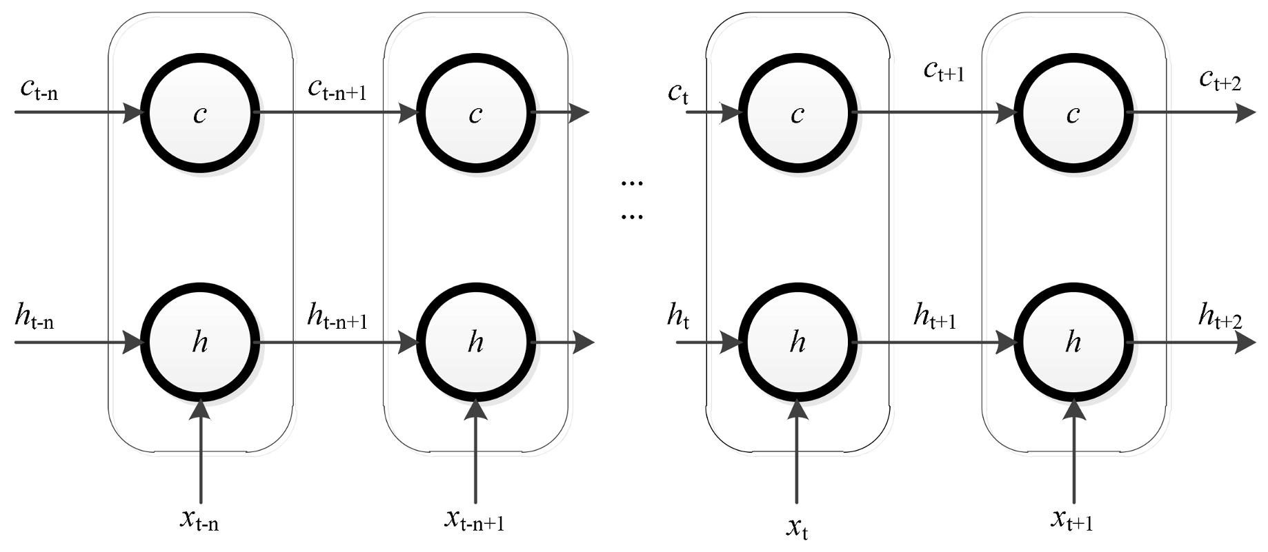
2.1. Long Short-Term Memory Networks

A simple recurrent neural network consists of an input layer, a hidden layer, and an output layer [17]. An input sequence is in the form x = (x₁, x₂, ..., x_t). After receiving input x_t at time t, the hidden layer state of the RNN is h_t and the output value is z_t. The calculation method is shown in Equations (1) and (2):

$$z_{\mathrm{t}}=\sigma (V{h}_{\mathrm{t}})$$

(1)

$$h_{\mathrm{t}}=f(U{x}_{\mathrm{t}}+W{h}_{\mathrm{t}-1})$$

(2)

where V is the weight matrix of the output layer, 𝜎(∙) is the activation function of the output layer, U is the weight matrix of the input x, W is the weight matrix of the hidden layer state h_t−1 at time t − 1 as the input at time t, and f(∙) is the hidden layer activation function.

Equations (1) and (2) are combined to calculate the result, as shown in Equation (3).

$$z_{\mathrm{t}}=Vf(U{x}_{\mathrm{t}}+Wf(U{x}_{\mathrm{t}-1}+Wf(U{x}_{\mathrm{t}-2}+Wf(U{x}_{\mathrm{t}-3}+\cdots ))))$$

(3)

From Equation (3), we can see that the output value z_t of the RNN is affected by all previous inputs x_t, x_t−1, x_t−2, x_t−3, ...

Due to the existence of the gradient dissipation and explosion problems [25], traditional RNNs are less effective at modeling long sequences. However, the LSTM network controls the instantaneous information impact on the historical information by adding memory cells and gate units [21] so that the network model can save and transmit information over a long time. The LSTM block structure at a single time step is shown in Figure 1.

At time t, the inputs of the LSTM are the sequence input value x_t at time t, the hidden layer value h_t−1 for the LSTM at time t − 1, and the state c_t−1 for the memory cell at time t − 1. The outputs of the LSTM are the hidden layer value h_t at time t and the memory cell state c_t at time t. In the LSTM, the forget gate determines the impact of c_t−1 on c_t, the input gate determines the impact of x_t on c_t, and the output gate controls the impact of c_t on h_t. The forget gate, input gate, and output gate are calculated using Equations (4)–(6), respectively:

$$f_{\mathrm{t}}=\sigma (W_{\mathrm{f}}\cdot [h_{\mathrm{t}-1},x_{\mathrm{t}}]+b_{\mathrm{f}})$$

(4)

$$i_{\mathrm{t}}=\sigma (W_{\mathrm{i}}\cdot [h_{\mathrm{t}-1},x_{\mathrm{t}}]+b_{\mathrm{i}})$$

(5)

$$o_{\mathrm{t}}=\sigma (W_{\mathrm{o}}\cdot [h_{\mathrm{t}-1},x_{\mathrm{t}}]+b_{\mathrm{o}})$$

(6)

where f_t, i_t, and o_t are the states of the forget gate, input gate, and output gate, respectively; σ(∙) is the activation function; W_f, W_i, and W_o are the weight matrices of the forget gate, input gate, and output gate, respectively; and b_f, b_i, and b_o are the bias items of the forget gate, input gate, and output gate, respectively.

The final output of the LSTM is determined by the state of the output gate and the memory cell, as follows:

$$\{\begin{array}{l}{c}_{\mathrm{t}}=f_{\mathrm{t}}\odot c_{\mathrm{t}-1}+i_{\mathrm{t}}\odot \tanh (W_{\mathrm{c}}\cdot [h_{\mathrm{t}-1},x_{\mathrm{t}}]+b_{\mathrm{c}})\\ h_{\mathrm{t}}=o_{\mathrm{t}}\odot \tanh (c_{\mathrm{t}})\end{array}$$

(7)

where W_c is the weight matrix of the input memory cell state, b_c is the bias item of the input memory cell state, and ⊙ denotes element-wise multiplication. Figure 2 shows the unrolled LSTM sequential architecture.

The accumulation of historical information depends not on the hidden state h itself but on the memory cell self-connection. In accumulation processing, the most recent moment of the memory cell information is limited by the forget gates, and the additional information relies on the input gate for restriction.

2.2. Backpropagation through Time Algorithm

The LSTM networks adopt the Backpropagation through Time (BPTT) algorithm [26] for training. It consists of the following steps: (1) Forward calculate the output value of each neuron. (2) Backward calculate the error term δ for each neuron. The back propagation for the LSTM includes backpropagation through time and backpropagation layer-wise. (3) Update the gradient of each weight based on the corresponding error term.

By setting a specific target between the output and the input characteristic parameters, LSTM networks automatically extract the correlation between the parameters throughout the training to acquire the prediction or classification. The LSTM network has three gate units to protect and control the cell status. The input, forget, and output gates correspond to the injection, accumulation, and output, respectively, of the transformer-related state parameters. The gate units realize the memory function in time to prevent gradient dissipation or explosion. The deep structure provides a foundation for mining the relationship between the various state parameters.

3. Transformer Operating State Prediction Using the LSTM-Based Approach

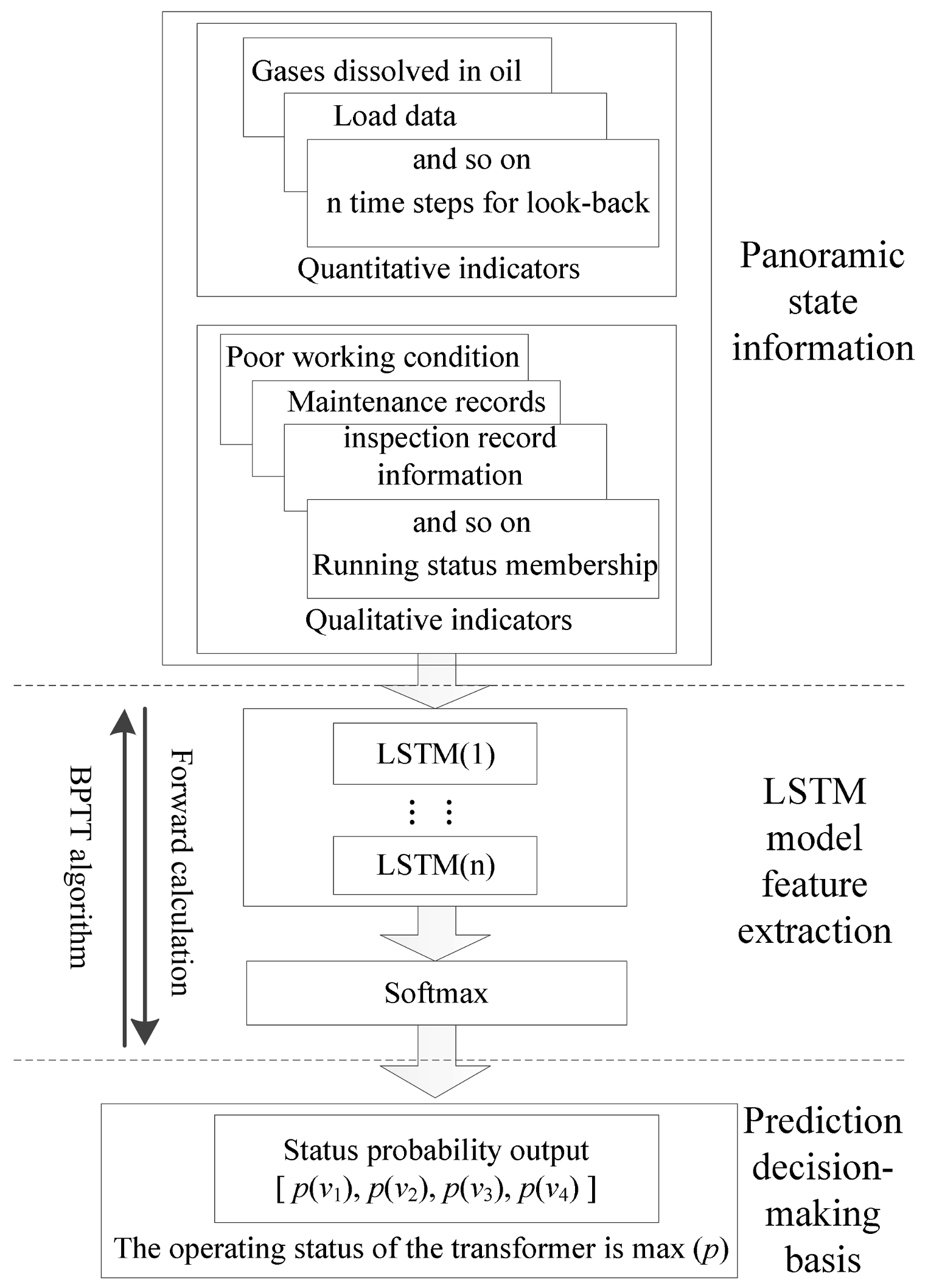
3.1. Input Characteristic Parameters Based on Panoramic Information

The relevant data needed for the research were provided by State Grid Corporation of China (Beijing, China). The voltage levels of the transformers are from 35 kV to 750 kV. Among them, the transformers appearing in the historical fault data are from across the 28 provinces in China, and the transformers were put into operation starting in the year 1989. Information relating to the defects and fault cases includes the basic transformer account information, inspection record information, poor working condition records, defects and fault dates, defect types, causes, disassembly photos, the corresponding routine test and diagnostic test data, H₂, CO, CO₂, CH₄, C₂H₄, C₂H₂, C₂H₆, gas production rates, main gas ratios (C₂H₂/C₂H₄, CH₄/H₂, C₂H₄/C₂H₆, CO₂/CO), corresponding load data (active and reactive power), and the corresponding meteorological data (temperature, humidity, sunlight intensity, wind speed, rainfall, and snowfall).

In the above database, there are two categories of data for assessing and predicting the transformer operating state: quantitative and qualitative indicators. Quantitative indicators represent data with different dimensions and magnitudes, and qualitative indicators represent the state in descriptive language. Qualitative indicators cannot be used directly in the assessment of the transformer status and must be quantified for calculation. The following section introduces the specific quantification method used.

3.2. Output Target Defined from the Transformer Operating Status

In general, the transformer operating state is divided into four patterns: normal operating state, minor defects, severe defects, and critical state [27]. The corresponding set of states is V = {v₁, v₂, v₃, v₄} = {good, poor, severe, and worst}.

v₁ indicates that the equipment is stable and that all the state parameters are in accordance with the standard. v₂ indicates that some of the parameters of the trend are approaching the direction of the standard limit but have not exceeded the standard and that the transformer can continue to run. v₃ indicates that some of the characteristic parameters have changed significantly and are close to the standard limit or that some of the parameters exceed the standard limit. v₄ indicates that some of the characteristic parameters have exceeded the standard limit and manifested as one or more critical defects. Power outage maintenance must be arranged immediately.

Table 1. Transformer running status and corresponding maintenance strategy.

Symbol	Running Status	Maintenance Strategy
v1	good	Planned maintenance
v2	poor	Priority maintenance
v3	severe	Maintenance as soon as possible
v4	worst	Immediate maintenance

shows the operating state of a transformer and the corresponding maintenance strategy.

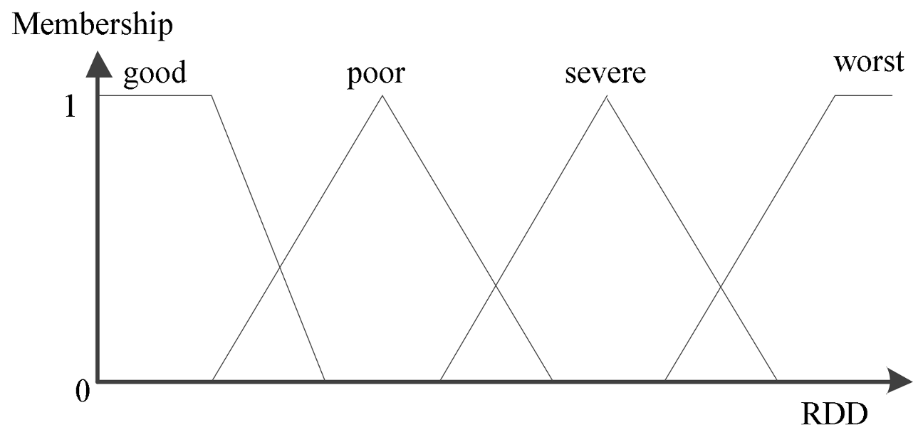
3.3. Methods for Indicator Quantification

In this paper, the relative degree of degradation (RDD) [28] is used to characterize the current state of the transformer compared to the fault state. The RDD reflects the degree of conversion of the transformer state from normal to fault patterns, and is expressed as a value in [0, 1]. The smaller the value is, the better the state is. A value of 0 indicates that the transformer is in good and normal condition, and a value of 1 signifies that the transformer is in the critical fault condition.

The optimal value of the parameter in the quantitative index is a, the alarm value is b, and the current measured value is d. The RDD of the indicator can be expressed as

$$r(d)=G(a,b,d)$$

(8)

where r represents the RDD of the indicator and G represents the deterioration function.

In this paper, the quantitative indicator function of the transformer status is established from the perspective of natural degradation. For the maximal indicators, such as the absorption ratio, the larger the data are, the better the state is. For the minimal indicators, such as gases dissolved in the insulation oil, the smaller the data are, the better the state is. The RDDs of the extremely large indicator and minimal indicator are respectively expressed by

$$r_l(d)=\{\begin{array}{l} 0 , d\ge a_l\\ (a_l-d)/(a_l-b_l),b_l<d<a_l\\ 1 , d\le b_l\end{array}$$

(9)

$$r_m(d)=\{\begin{array}{l} 1 , d\ge b_m\\ (d-a_m)/(b_m-a_m),a_m<d<b_m\\ 0 , d\le a_m\end{array}$$

(10)

where r_l and r_m represent the RDDs of the extremely large indicator and minimal indicator, respectively; a_l and a_m represent the optimal values of the extremely large indicator and minimal indicator, respectively; b_l and b_m represent the alarm values of the extremely large indicator and minimal indicator, respectively; and d represents the current measured value.

For quantitative data, we use the fuzzy distribution method to establish the mapping of each indicator corresponding to different operating states. The triangular–trapezoid combination membership function has a simple distribution and intuitive results [27]. The triangular–trapezoid model is in accordance with the four types of power transformer operating states [29]. Taking the quantitative monitoring data as the input characteristic parameter and the RDD as the output target, the support vector machine (SVM) has a strong ability to address small sample data and is used to fit the distribution function, as shown in Figure 3.

For qualitative indicators using descriptive language, such as manual inspection records and some technical performance parameters, we used a fuzzy statistical experiment to determine the membership. First, a number of experts gave the basis of the evaluation criteria and set the score range as [0, 100]. The higher the score is, the worse the degree of deterioration is. Then, the score was normalized to [0, 1] to determine the degree of membership. Based on the relative importance of job title, seniority, and academic qualifications, which are related to the level of technical experience, experts were given different weights to reduce the subjective influence on the quantitative results. The data set provided by the State Grid Corporation of China is relatively complete and there is no missing input information. The weighted scoring mechanism is given by:

$$l_i={\displaystyle {\sum }_j^n{l}_{ij}}{w}_j$$

(11)

where l_i is the score for different state levels of indicator i, l_ij is the score for different state levels of indicator i given by the jth expert, and w_j is the weight of the jth expert. The weights satisfy the relationship ∑w_j = 1, and the total number of experts is n.

In the comprehensive state evaluation of the transformer, the contribution of each indicator is different. Different weights can distinguish the importance of the indicator. Therefore, determining the weights reasonably is the key to an accurate assessment. In view of the complexity of the transformer system and to minimize the subjective factors, the analytic hierarchy process (AHP) [29] was used to give weights to each indicator.

By using the above quantitative process, we can assess the health index of the transformer and ultimately determine the transformer operating state. This can allow us to revise and supplement the labels for the operating state of the transformers.

3.4. The Proposed LSTM Prediction Model

The transformer panoramic state information is taken as the input characterization parameters. From the information, the quantitative data are normalized, and the qualitative information is transformed into state membership. The state probability interval to be predicted at the next moment is taken as the output. Through nonlinear transformations and LSTM correlation feature extraction, the Softmax classifier predicts the probability of the next moment to determine the state of the transformer. Figure 4 shows the transformer state prediction architecture based on the LSTM network. The detailed steps are given below.

(1)

Samples are collected and divided into training sets and test sets.

(2)

To reduce the influence of the data dispersion, quantitative data are normalized using the standard deviation method:

$${\overline{d}}_k=(d_k-d_{\min k})/(d_{\max k}-d_{\min k})$$

(12)

where d_{min k} is the minimum monitoring data of the indicator k, d_{max k} is the maximum monitoring data of the indicator k, and d_k is the monitoring data of the indicator k.

(3)

Quantitative data is fit to the membership function of the RDD and operating state using the SVM.

(4)

Qualitative indicators are quantified according to the fuzzy statistical experiment.

(5)

The AHP method is used to determine the weight of each indicator.

(6)

The comprehensive fuzzy evaluation results corresponding to v₁–v₄ are weighted with Steps (3) and (4) according to Step (5), and the comprehensive evaluation results are taken as the LSTM output labels.

(7)

According to the BPTT algorithm, the LSTM network model is trained to extract the feature relationships between the key parameters and the predicted transformer status, and the parameters of the prediction model are obtained.

(8)

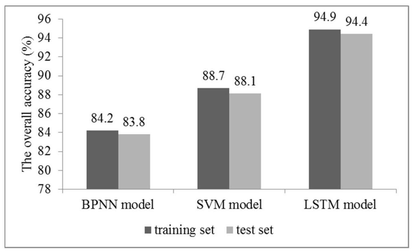
The prediction parameters of the LSTM model are used to predict the operating state of the transformer in the test set, and the accuracy of the model is verified.

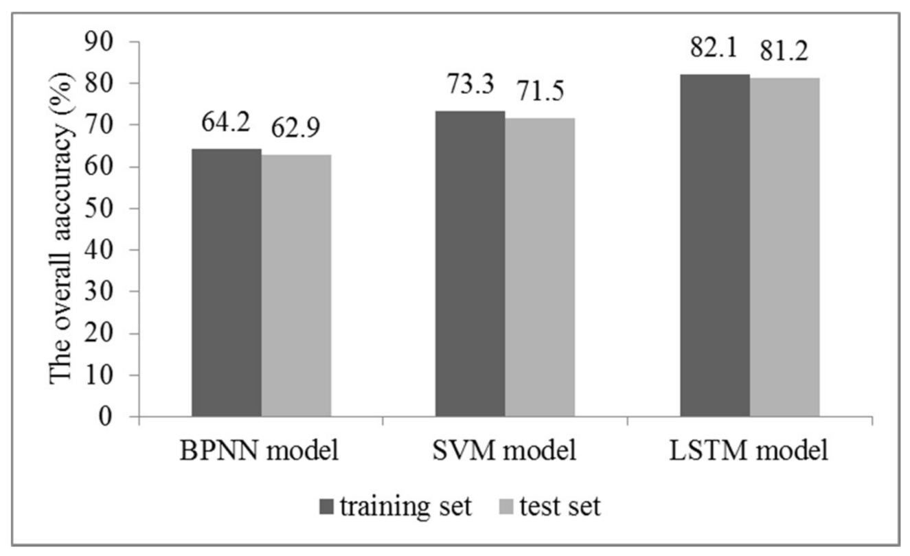
4. Case Studies and Analysis

A total of 206 transformers showing confirmed existence of abnormal defects/faults and 174 transformers indicating early warnings/alarms from the oil chromatographic online monitoring devices formed the sample library of the prediction model. According to the data from the 380 transformers in the sample database, 228 transformers were randomly selected to form the training set, and the remaining 152 transformers were used to form the test set. The LSTM networks were used to extract the correlation between the predicted transformer state and the panoramic information.

To increase the learning speed and reduce the risk of the network falling into the local minimum, the weight matrix in the LSTM was initialized using a Gaussian distribution with a mean of 0 and variance of 1, and the quadrature matrix was obtained from the singularity decomposition value [30]. The LSTM bias term and the output layer bias were initialized to 0. The output layer weight matrix was multiplied by 0.01 for the random number from the Gaussian distribution with a mean of 0 and variance of 1. The input layer size of the prediction was 72, the number of LSTM hidden layer neurons was 100, and the output layer size was 4. To prevent over-fitting, the signal loss rate was set to 0.2.

Meanwhile, with the same input characteristic parameters and output targets, the support vector machine (SVM) and backpropagation neural network (BPNN) model were constructed to predict the transformer operating state using the training samples. The SVM model used the radial basis function (RBF) as the kernel. The optimal penalty factor was 0.1, and the RBF kernel parameter was 10⁻³, as obtained through cross-validation. The structure of the BPNN consisted of an input layer, a hidden layer, and an output layer. By using a trial and error method, the optimal number of neurons in each layer was chosen to be 72, 200, and 4, respectively. The learning rate in the BPNN model was 0.03, and the learning cycle was 1000. The prediction models were based on the Python language in an Ubuntu 15 operating environment.

To evaluate the performance of the prediction model, we used the overall average accuracy. Accuracy expresses the probability that the result for each random sample predicted using the model matches the actual type. The overall average accuracy is defined as

$$A=\frac{N_{\mathrm{P}}}{N_{\mathrm{T}}}\times 100\%$$

(13)

where N_P denotes the number of correctly predicted samples and N_T denotes the total number of samples in the entire dataset.

The relationship between the quantitative data represented by the dissolved gas in the oil and the operating state is calculated as follows. The RDDs of H₂, CH₄, C₂H₄, C₂H₆, C₂H₂, CO/CO₂, and total hydrocarbons are taken as the input characteristic parameters, and the operating state is the output target. A least squares support vector machine (LS-SVM) was used to fit the distribution function.

The fitting sample database was composed of the off-line experimental dissolved gas analysis (DGA) data of 206 transformers, which showed confirmed existence of abnormal defects/faults. The sample data included the monitoring information from the equipment normal operation period, deterioration period, and fault, and they dynamically characterized the trend of the equipment status. Of these, 137 cases were used for training, and 69 cases were used for testing. The operating states of 66 samples in the test set were predicted with an accuracy rate of 95.7%. The RDD of the gases dissolved in the oil corresponds to the v₁–v₄ membership functions ${\varphi }_{v_{\mathrm{i}}}(r)$, as follows.

$${\varphi }_{v_1}(r)=\{\begin{array}{l} 1 , r<0.218\\ -5.155r+2.124, 0.218\le r\le 0.412\\ 0 , r>0.412\end{array}$$

(14)

$${\varphi }_{v_2}(r)=\{\begin{array}{l} 5.155r-1.124,0.218<r\le 0.412\\ -0.515r+3.124 ,0.412<r\le 0.606\\ 0 , r>0.606\mathrm{or}r<0.218\end{array}$$

(15)

$${\varphi }_{v_3}(r)=\{\begin{array}{l} 5.155r-2.124 , 0.412<r\le 0.606\\ -5.155r+4.124, 0.606<r\le 0.8\\ 0 , r>0.8\mathrm{or}r<0.412\end{array}$$

(16)

$${\varphi }_{v_4}(r)=\{\begin{array}{l} 0 , r<0.606\\ 5.155r-3.124, 0.606\le r\le 0.8\\ 1 , r>0.8\end{array}$$

(17)

We take the linguistic description of the maintenance history as an example to provide quantitative results of the qualitative variable. The results are shown in

Table 2. Account of transformer maintenance history.

Index	Maintenance History
0–0.25	Maintenance work has no difficulty. Maintenance frequency is not very high, and no defect is left untreated.
0.25–0.5	Maintenance work has slight difficulty. Maintenance frequency is not high, and a small defect is left untreated.
0.5–0.75	Maintenance work has some difficulty. Maintenance frequency is high, and a few defects are left untreated.
0.75–1	Maintenance work is very difficult. Maintenance frequency is higher, and obvious defects/faults are left untreated.

.

Five experts were invited to give the relative importance of the comparison between the indicators according to the AHP requirements. We used these data to calculate the weights. The traditional method is to construct a judgment matrix and find the maximum eigenvalues of the matrix and the corresponding eigenvectors. The eigenvectors are the index weights. However, in practice, the construction of the evaluation matrix is only adjusted based on a rough estimate. It is arbitrary and often requires multiple adjustments to satisfy the consistency check. An improved method [31] can be adopted to calculate the optimal transfer matrix to naturally meet the consistency, and the relative weight of each evaluation factor can be obtained directly. The calculation results are shown in

Table 3. Weight of each indicator.

Indicator	Weight	Indicator	Weight
Gas dissolved in oil	0.335	Corrosive gases and dust	0.0055
Dielectric loss value	0.168	Altitude and wind speed	0.0076
Core earthing current	0.1023	Load condition	0.0068
Moisture content	0.1202	Running temperature	0.0189
Dielectric loss of oil	0.1058	Abnormal noise	0.0024
Breakdown voltage	0.0597	Nearby short-circuit	0.0147
Air temperature	0.0034	Protection action	0.012
Air humidity	0.0041	Maintenance history	0.0345

, and the specific calculation process can be found elsewhere [31].

In this work, we adopted the weighted average of the comprehensive evaluation. The element v_i corresponding to the maximum evaluation value is determined as the evaluated operating state. The assessment results are the labels used to construct the prediction models.

4.1. Short-Term Prediction of the Transformer Operating State

To evaluate the short-term prediction performance of the three models, experiments with a forecast horizon of one week were implemented. The overall average accuracies generated from the different models for the training and test datasets are shown in Figure 5.

Based on the prediction results, the accuracies with the prediction horizon of one week clearly increase over BPNN, SVM, and LSTM models, in that order. The accuracy of the LSTM model is increased significantly by 10.7% and 6.2% compared with those of the BPNN and SVM models, respectively. The test accuracy is increased by 10.6% and 6.3%, respectively.

Taking the 500 kV #2 transformer as an example, the basic condition of the transformer is as follows. The date of production is July 2006 and the date of initial operation is November 2006. Routine tests on 19 March 2008 and 26 May 2011 showed no abnormalities. The transformer top oil temperature varies in the range of 30~60 °C. In the summer of 2009, it suffered a lightning over-voltage, and a defect occurred. The running environment is harsh, and the pollution level is II. The poor working condition records show that a 30% overload lasted for 43 min on 18 July 2011. The on-line monitoring data of the oil chromatography from 14 to 26 March 2012 are shown in

Table 4. Oil chromatography online monitoring data for the 500 kV #2 transformer (units: µL/L).

Date	H2	CH4	C2H4	C2H6	C2H2	TH	CO	CO2
14 March	32.77	10.29	4.56	1.64	0.13	16.62	176.3	693.1
15 March	36.58	10.46	4.87	1.57	0.15	17.05	178.7	698.6
16 March	34.89	9.98	4.33	1.71	0.15	16.17	168.5	704.8
17 March	33.21	10.9	4.72	1.68	0.16	17.46	174	707.9
18 March	35.76	10.32	4.28	1.75	0.17	16.52	185.4	697.1
19 March	38.63	10.65	4.64	1.8	0.14	17.23	171.7	701.7
20 March	40.52	10.44	4.39	1.95	0.18	16.96	180.5	682.3
21 March	37.97	10.88	4.61	1.89	0.17	17.55	183	709.3
22 March	34.51	10.49	5.09	1.71	0.22	17.51	185.9	715.1
23 March	35.39	10.61	4.68	1.74	0.21	17.24	180	724.8
24 March	37.28	10.4	4.44	1.89	0.23	16.96	178.8	715.4
25 March	55.07	15.05	12.71	4.4	0.48	32.64	184.3	720.6
26 March	70.17	18.89	17.04	6.9	0.61	43.44	185.3	717

.

The data from 14 to 26 March 2012 are used to predict the operating state of the transformer one week later, on 2 April 2012. The probabilities predicted from the BPNN, SVM, and LSTM models corresponding to states v₁–v₄ are [0.2434, 0.6166, 0.1700, 0], [0, 0.4356, 0.4419, 0.1225], and [0, 0.0191, 0.7308, 0.2501], respectively. According to the principle of maximum confidence, the BPNN prediction result corresponds to a v₂ (or poor) state. The SVM prediction result corresponds to a v₃ (or severe) state, with a small difference between the v₂ and v₃ state reliabilities, indicating that the prediction recognition effect is not distinct. The LSTM prediction results correspond to the v₃ (or severe) state, with an obvious identification effect.

On 2 April 2012, the content of H₂ dissolved in the oil reached 185.76 µL/L and the content of C₂H₂ reached 2.98 µL/L. The online monitoring system was activated. Then, the ultrasonic partial discharge test of the transformer was carried out, and an internal discharge phenomenon was found. During the overhaul of this transformer, the maintenance personnel found that overhang angle of the silicon steel sheet on the transformer core iron yoke parts exhibited severe deformation, as shown in Figure 6. The protrusive tips of the overhang angles in magnetic fields vibrated strongly and caused the contact discharge, resulting in the abnormal content of dissolved gases in the transformer oil. The discharge did not affect the solid insulation, so the contents of CO and CO₂ exhibited no significant change. The predicted results of the LSTM model are consistent with the actual transformer running status.

4.2. Long-Term Prediction of the Transformer Operating State

To evaluate the long-term prediction performance of the three models, experiments with a forecast horizon of one month were implemented. The results are shown in Figure 7.

Compared with Figure 5, with an increase in the prediction horizon, the prediction accuracies of the three models are reduced. As seen from Figure 7, the accuracies with the prediction horizon of one month ranked in the order of BPNN, SVM, and LSTM from worst to best. Compared with the BPNN and SVM models, the accuracy of the LSTM model in the training set is increased by 17.9% and 8.8%, respectively, and the accuracy of test set is increased by 18.3% and 9.7%, respectively.

Taking a 220 kV #1 transformer as an example, the basic condition of the transformer is as follows. The date of production is April 2000, and the date of initial operation is June 2000. The transformer is in basically good operation, and the overall load rate is relatively high. The chromatographic period detection found that the total hydrocarbon content of the transformer in 2010, after meeting the peak demands in the summer, had a greater increase. Subsequently, the total hydrocarbon content slowly increased year after year but did not exceed the alarm value. Except for the total hydrocarbons, the remaining characteristic gases dissolved in the insulation oil were normal. Some of the oil chromatography online monitoring data from June to July 2013 are shown in

Table 5. Oil chromatography online monitoring data for the 220 kV #1 transformer (units: µL/L).

Date	H2	CH4	C2H4	C2H6	C2H2	TH	CO	CO2
15 June	2.67	58.35	22.75	23.59	0	104.69	110.2	516.3
26 June	2.37	66.35	23.28	25.14	0	114.76	116.4	522.6
7 July	2.67	78.70	20.6	22.35	0	121.64	117.0	519.8
15 July	2.37	86.05	20.68	22.19	0	128.93	108.1	514.7
24 July	2.37	99.69	20.15	21.89	0	141.73	102.4	510.8

.

The data from June to July 2013 were used to predict the operating state of the transformer one month later, on August 2013. As the load rate of this transformer is special, we consider both the under-load and full-load cases in the predictions.

In the under-load condition, the probabilities predicted from the BPNN, SVM, and LSTM models corresponding to states v₁–v₄ are [0.0027, 0.2956, 0.5711, 0.1306], [0, 0.2735, 0.5172, 0.2093], and [0, 0.1038, 0.6096, 0.2866], respectively. The BPNN, SVM, and LSTM model prediction results all correspond to the v₃ (severe) state. We predict that there should be a severe fault inside the transformer. Although the transformer can continue to run, operation and maintenance personnel should arrange maintenance work as soon as possible.

In the full-load condition, the probabilities predicted from the BPNN, SVM, and LSTM models corresponding to states v₁–v₄ are [0, 0.2173, 0.2748, 0.5079], [0, 0.1985, 0.2561, 0.5454] and [0, 0.1835, 0.2149, 0.6016], respectively. The BPNN, SVM, and LSTM model prediction results all correspond to the v₄ (the worst) state. Thus, the transformer needs to be repaired immediately.

In fact, the operation and maintenance personnel in the substation contacted the dispatching department and prohibited the operation of this transformer under full-load conditions. After the summer, during the overhaul of this transformer, the maintenance personnel found that a severe overheating fault had occurred under part of the clamp and tank potential connection. There were more obvious signs of overheating discoloration. For the controlling load, the fault of this transformer had not yet entered the critical worst running conditions.

5. Conclusions

This paper studied the status of early warning technologies for power transformers and proposed a transformer operating state prediction method based on the data-driven LSTM network. The conclusions are as follows.

(1) By analyzing the state panoramic information of the transformer, the degree of deterioration of the transformer is depicted in the RDD. The membership relationship between the RDD of each indicator and the state of the transformer is obtained using fuzzy treatment. Then, the LSTM network is constructed to automatically extract the feature relationship between each indicator and the predicted operating state.

(2) The case studies show that the proposed method can effectively predict the operating state of power transformers. The model based on LSTM networks predicts the state of the transformer with an accuracy of 94.4% for a one-week forecast horizon and 81.2% for a one-month forecast horizon. Compared with the traditional BPNN and SVM methods, the LSTM model can more accurately reflect the real situation of the transformers.

(3) By predicting and analyzing the operating state of the transformers, the prediction results based on the LSTM network are in accordance with the actual conditions. The difference in the predicted state probabilities is more obvious, and the results are more convincing.

We will focus on improving the LSTM model in future research. The deep learning methods will be combined with intelligent optimization algorithms to determine the optimal parameters of the prediction model.

References

1. Kelly, J.J.; Myers, D.P. Transformer life extension through proper reinhibiting and preservation of the oil insulation. IEEE Trans. Ind. Appl. 2015, 31, 56–60. [Google Scholar] [CrossRef]
2. Liao, R.J.; Bian, J.P.; Yang, L.J.; Grzybowski, S.; Wang, Y.Y.; Li, J. Forecasting dissolved gases content in power transformer oil based on weakening buffer operator and least square support vector machine—Markov. IET Gener. Transm. Distrib. 2012, 6, 142–151. [Google Scholar] [CrossRef]
3. Liao, R.J.; Zheng, H.B.; Grzybowski, S.; Yang, L.J.; Tang, C.; Zhang, Y.Y. Fuzzy information granulated particle swarm optimisation-support vector machine regression for the trend forecasting of dissolved gases in oil-filled transformers. IET Electr. Power Appl. 2011, 5, 230–237. [Google Scholar] [CrossRef]
4. He, Q.; Si, J.; Tylavsky, D.J. Prediction of top-oil temperature for transformers using neural networks. IEEE Trans. Power Deliv. 2000, 15, 1205–1211. [Google Scholar] [CrossRef]
5. Yang, W.; Liu, Z.Z.; Chen, H.X. Research on residual flux prediction of the transformer. IEEE Trans. Magn. 2017, 53, 6100304. [Google Scholar] [CrossRef]
6. Wang, F.H.; Geng, C.; Su, L. Parameter identification and prediction of Jiles—Atherton model for DC-biased transformer using improved shuffled frog leaping algorithm and least square support vector machine. IET Electr. Power Appl. 2015, 9, 660–669. [Google Scholar] [CrossRef]
7. Cardelli, E.; Faba, A.; Tissi, F. Prediction and control of transformer inrush currents. IEEE Trans. Magn. 2015, 51, 1–4. [Google Scholar] [CrossRef]
8. Baral, A.; Chakravorti, S. Prediction of moisture present in cellulosic part of power transformer insulation using transfer function of modified debye model. IEEE Trans. Dielectr. Electr. Insul. 2014, 21, 1368–1375. [Google Scholar] [CrossRef]
9. Shaban, K.B.; El-Hag, A.H.; Benhmed, K. Prediction of Transformer Furan Levels. IEEE Trans. Power Deliv. 2016, 31, 1778–1779. [Google Scholar] [CrossRef]
10. Qiu, J.; Wang, H.F.; Lin, D.Y.; He, B.T.; Zhang, W.F.; Xu, W. Nonparametric regression-based failure rate model for electric power equipment using lifecycle data. IEEE Trans. Smart Grid 2015, 6, 955–964. [Google Scholar] [CrossRef]
11. Chowdhury, A.A.; Koval, D.O. Development of probabilistic models for computing optimal distribution substation spare transformers. IEEE Trans. Ind. Appl. 2005, 41, 1493–1498. [Google Scholar] [CrossRef]
12. Zhou, D.; Wang, Z.; Li, C. Data requisites for transformer statistical lifetime modelling—Part I: Aging-related failures. IEEE Trans. Power Deliv. 2013, 28, 1750–1757. [Google Scholar] [CrossRef]
13. Tokunaga, J.; Koide, H.; Mogami, K.; Hikosaka, T. Gas generation of cellulose insulation in palm fatty acid ester and mineral oil for life prediction marker in nitrogen-sealed transformers. IEEE Trans. Dielectr. Electr. Insul. 2017, 24, 420–427. [Google Scholar] [CrossRef]
14. Bakar, N.A.; Abu-Siada, A. Fuzzy logic approach for transformer remnant life prediction and asset management decision. IEEE Trans. Dielectr. Electr. Insul. 2016, 23, 3199–3208. [Google Scholar] [CrossRef]
15. Wouters, P.A.A.F.; van Schijndel, A.; Wetzer, J.M. Remaining lifetime modeling of power transformers: Individual assets and fleets. IEEE Electr. Insul. Mag. 2011, 27, 45–51. [Google Scholar] [CrossRef]
16. Sheng, G.; Hou, H.; Jiang, X.; Chen, Y. A novel association rule mining method of big data for power transformers state parameters based on probabilistic graph model. IEEE Trans. Smart Grid 2018, 9, 695–702. [Google Scholar] [CrossRef]
17. Mandic, D.P.; Chambers, J.A. Recurrent Neural Networks for Prediction: Learning Algorithms, Architectures and Stability; John Wiley: New York, NY, USA, 2001; pp. 31–46. [Google Scholar]
18. Xu, C.; Wang, G.; Liu, X.; Guo, D.; Liu, T.Y. Health Status Assessment and Failure Prediction for Hard Drives with Recurrent Neural Networks. IEEE Trans. Comput. 2016, 65, 3502–3508. [Google Scholar] [CrossRef]
19. Tian, Z.; Zuo, M.J. Health condition prediction of gears using a recurrent neural network approach. IEEE Trans. Reliab. 2010, 59, 700–705. [Google Scholar] [CrossRef]
20. Hochreiter, S.; Schmidhuber, J. Long short-term memory. Neural Comput. 1997, 9, 1735–1780. [Google Scholar] [CrossRef] [PubMed]
21. Graves, A.; Mohamed, A.; Hinton, G. Speech recognition with deep recurrent neural networks. In Proceedings of the 2013 IEEE International Conference on Acoustics, Speech and Signal Processing (ICASSP), Vancouver, BC, Canada, 26–30 May 2013; IEEE: Vancouver, BC, Canada; pp. 6645–6649. [Google Scholar]
22. Zheng, S.; Ristovski, K.; Farahat, A.; Gupta, C. Long Short-Term Memory Network for Remaining Useful Life estimation. In Proceedings of the 2017 IEEE International Conference on Prognostics and Health Management (ICPHM), Dallas, TX, USA, 19–21 June 2017; IEEE: Ottawa, ON, Canada; pp. 88–95. [Google Scholar]
23. Kong, W.; Dong, Z.Y.; Jia, Y.; Hill, D.J.; Xu, Y.; Zhang, Y. Short-term residential load forecasting based on lstm recurrent neural network. IEEE Trans. Smart Grid 2017, 1. [Google Scholar] [CrossRef]
24. Wang, H.; Lin, A.D.; Qiu, J.; Ao, L.; Du, Z.; He, B. Research on multiobjective group decision-making in condition-based maintenance for transmission and transformation equipment based on DS evidence theory. IEEE Trans. Smart Grid 2015, 6, 1035–1045. [Google Scholar] [CrossRef]
25. Bengio, Y.; Simard, P.; Frasconi, P. Learning long-term dependencies with gradient descent is difficult. IEEE Trans. Neural Netw. 1994, 5, 157–166. [Google Scholar] [CrossRef] [PubMed]
26. Schmidhuber, J. A fixed size storage O (n3) time complexity learning algorithm for fully recurrent continually running networks. Neural Comput. 1992, 4, 243–248. [Google Scholar] [CrossRef]
27. Ranga, C.; Chandel, A.K.; Chandel, R. Condition assessment of power transformers based on multi-attributes using fuzzy logic. IET Sci. Meas. Technol. 2017, 11, 983–990. [Google Scholar] [CrossRef]
28. Li, L.; Cheng, Y.; Xie, L.J.; Jiang, L.Q.; Ma, N.; Lu, M. An integrated method of set pair analysis and association rule for fault diagnosis of power transformers. IEEE Trans. Dielectr. Electr. Insul. 2015, 22, 2368–2378. [Google Scholar] [CrossRef]
29. Sun, L.; Ma, Z.; Shang, Y.; Liu, Y.; Yuan, H.; Wu, G. Research on multi-attribute decision-making in condition evaluation for power transformer using fuzzy AHP and modified weighted averaging combination. IET Gener. Transm. Distrib. 2016, 10, 3855–3864. [Google Scholar] [CrossRef]
30. Zhou, J.; Xu, W. End-to-end learning of semantic role labeling using recurrent neural networks. In Proceedings of the 53rd Annual Meeting of the Association for Computational Linguistics and the 7th International Joint Conference on Natural Language Processing, Beijing, China, 27–31 July 2015; pp. 1127–1137. [Google Scholar]
31. Ma, Y.; Hu, M. Improved analysis of hierarchy process and its application to multi-objective decision. Syst. Eng. Theory Pract. 1997, 6, 40–44. (In Chinese) [Google Scholar]
Figure 1. The structure of a long short-term memory (LSTM) block.
Energies 11 00914 g001
Figure 2. The unrolled LSTM sequential architecture.
Energies 11 00914 g002
Figure 3. Function of power transformer operating state and relative degree of degradation (RDD).
Energies 11 00914 g003
Figure 4. Transformer operating state prediction architecture based on the LSTM. BPTT: Backpropagation through Time
Energies 11 00914 g004
Figure 5. Prediction accuracies of different models (prediction scale: one week). BPNN: backpropagation neural network. SVM: support vector machine.
Energies 11 00914 g005
Figure 6. The fault location of the transformer as found by maintenance.
Energies 11 00914 g006
Figure 7. Prediction accuracy of different models (prediction scale: one month).
Energies 11 00914 g007