Probabilistic Steady-State Operation and Interaction Analysis of Integrated Electricity, Gas and Heating Systems

Abstract

The existing studies on probabilistic steady-state analysis of integrated energy systems (IES) are limited to integrated electricity and gas networks or integrated electricity and heating networks. This paper proposes a probabilistic steady-state analysis of integrated electricity, gas and heating networks (EGH-IES). Four typical operation modes of an EGH-IES are presented at first. The probabilistic energy flow problem of the EGS-IES considering its operation modes and correlated uncertainties in wind/solar power and electricity/gas/heat loads is then formulated and solved by the Monte Carlo method based on Latin hypercube sampling and Nataf transformation. Numerical simulations are conducted on a sample EGH-IES working in the “electricity/gas following heat” mode to verify the probabilistic analysis proposed in this paper and to study the effects of uncertainties and correlations on the operation of the EGH-IES, especially uncertainty transmissions among the subnetworks.

1. Introduction

Conventionally, electricity, gas and heating networks are designed and operated independently as individual systems. The increasing application of combined heat and power units (CHP), gas-fired units and other energy conversion facilities (e.g., power to gas (P2G) and power to heat (P2H) equipment) enhance the degree of interdependence of different energy systems [1,2]. There is a growing interest in considering these multiple energy systems as an integrated whole, and the coordinated planning and operation of integrated energy systems (IES) to achieve the technical, economic, and environmental benefits from multiple energy utilization [3,4,5].

Steady-state modeling and analysis of an IES are usually considered to be the basis for its planning and operation. Many researchers have studied the steady-state analysis of the electricity-gas IES (i.e., IES composed of electricity and gas networks), the electricity-heat IES and the electricity-gas-heat IES. Zeng et al. [6] conducted a unified power- and gas-flow analysis of electricity-gas IES considering bi-directional energy conversion. Wang et al. [7] proposed a decomposed method for power and gas flow analysis to explore the impacts of gas composition on both electricity and gas networks. Considering the influence of environmental temperature on the pipelines and the gas network, Martinez-Mares et al. [8] proposed viewing the gas temperature as a state variable in modeling power and gas flow problems. Liu et al. [9,10] demonstrated the necessity for combined analysis of electricity and heating networks. Pan et al. [11] studied the physical interaction between electricity and heating networks. References [12,13,14] performed a steady-state energy-flow analysis of IES containing electricity, gas and heat based on the Newton-Raphson method. Clegg et al. [15] presented an integrated electricity-gas-heat transmission network model and applied it to the system in Great Britain. Cascio et al. [16] aimed for an urban EGH-IES and proposed an operational multi-objective optimization model. An integrated method for optimizing electricity, gas and heat in an EGH-IES was investigated in [17]. Although the references mentioned above have studied the steady-state analysis of electricity-gas IES [6,7,8], electricity-heat IES [9,10,11] and electricity-gas-heat IES [12,13,14,15,16,17], they are all deterministic analyses, in essence, and cannot address the effects of the uncertainties existing in an IES (e.g., loads and renewable energies) on the operation of IES.

Compared with conventional separated electricity, gas or heating networks, IES is exposed to more uncertain sources, such as intermittent renewable energy sources (wind, solar, etc.) and electricity/gas/heat loads. Moreover, uncertainties in IES are more complicated than in individual energy networks due to the mutual interaction among multiple energy networks. Any uncertain variation in one network may be transmitted to the other via coupling facilities (e.g., CHP unit, etc.), which may finally deteriorate the overall performance of the IES and even pose risks to the security of each energy network. It is therefore becoming a kind of necessity to perform the analysis of IES with the uncertainties considered carefully.

Probabilistic power flow analysis, which has been studied extensively, is a powerful tool for recognizing and evaluating the effects of uncertainties on electricity networks [18,19]. It is therefore logical and desirable to extend the probabilistic power flow technique to the multi-energy flow analysis of IES. Chen et al. [20,21] presented a probabilistic power and gas flow model considering uncertainties in wind speeds and electricity/gas/heat loads, and then solved the problem by Monte Carlo simulation (MCS). Hu et al. [22] applied the cumulant method and Gram-Charlier expansion to conduct probabilistic power and gas flow analysis. Yang et al. [23] investigated the effects of uncertainties and correlations in pipe parameters on power and gas flow of an electricity-gas IES. Sun et al. [24] studied probabilistic power and mass flow of combined electricity and heating networks considering uncertainties in photovoltaic power and electricity/heat loads.

Although the studies above [20,21,22,23,24] applied probabilistic techniques to perform probabilistic energy flow (PEF) analysis of IES, they have the following two limitations:

(1)

The existing studies are limited to the probabilistic analysis of electricity-gas IES [16,17,18,19] and electricity-heat IES [20]. To the best of our knowledge, studies on the PEF of the electricity-gas-heat IES are still not available in the published literature.

(2)

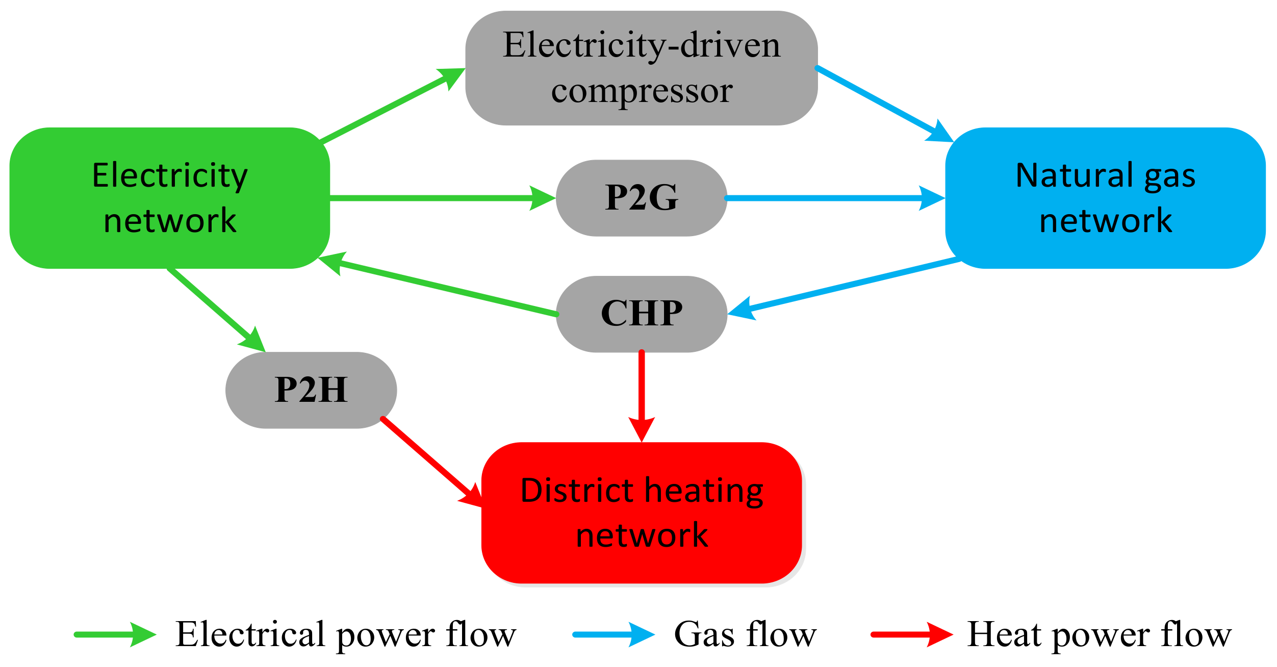
Interactions among different energy networks in an uncertain environment have not been thoroughly investigated by the existing studies. In fact, compared with the electricity-gas IES or electricity-heat IES, electricity-gas-heat IES will have more complicated interactions due to the tri-energy interdependency, necessitating further studies on interactions and their potential influences on the operation of IES.

Accordingly, this paper intends to study the probabilistic analysis of an electricity-gas-heat IES (EGH-IES) considering various operation modes and correlated uncertainties, and thus to disclose the effects of uncertainties and interactions on the operation of IES.

The contributions of this paper can be described as follows:

(1)

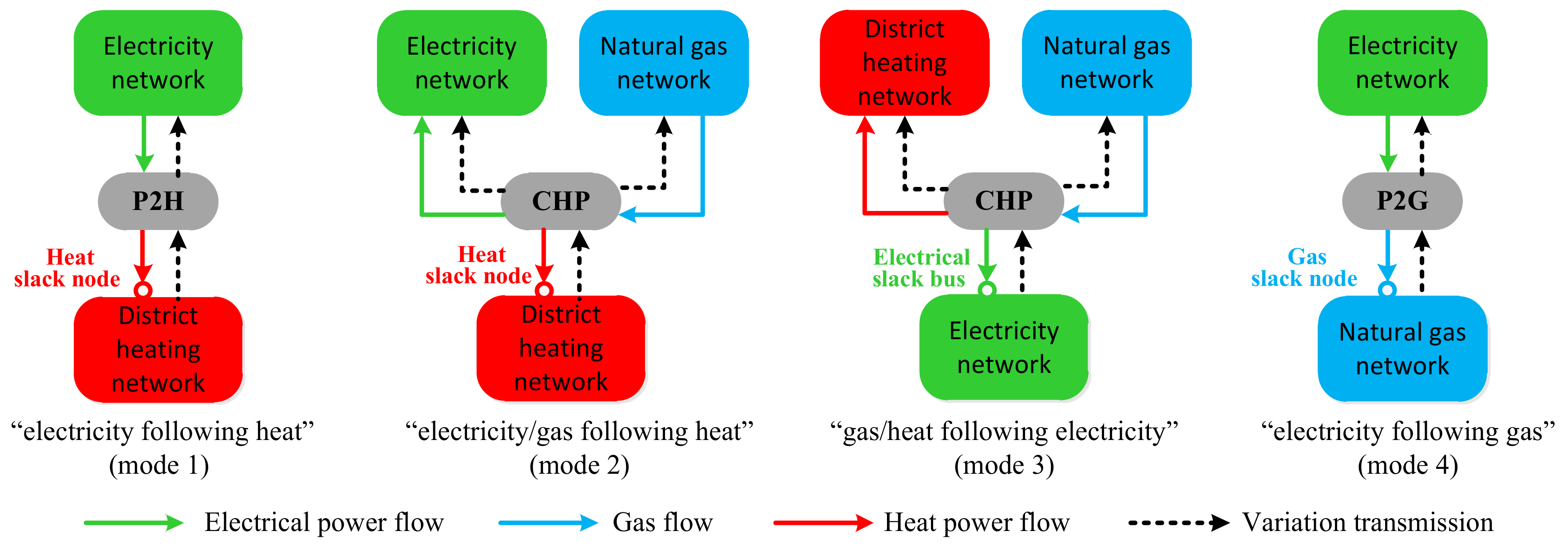
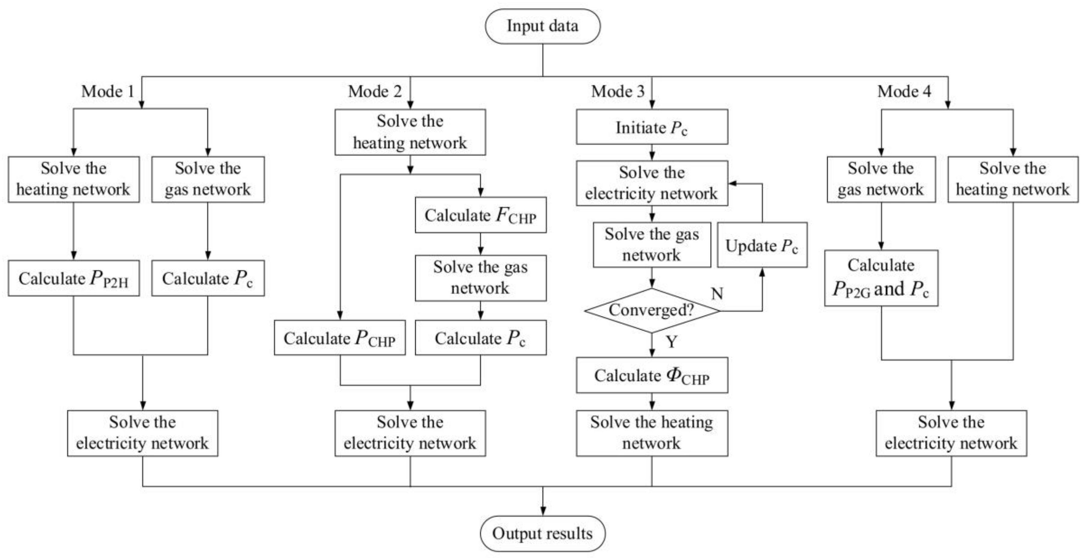
Four typical operation modes of an EGH-IES (i.e., “electricity following heat” mode, “electricity/gas following heat” mode, “gas/heat following electricity” mode and “electricity following gas” mode) are presented and discussed with a focus on the variation transmission among the three subnetworks.

(2)

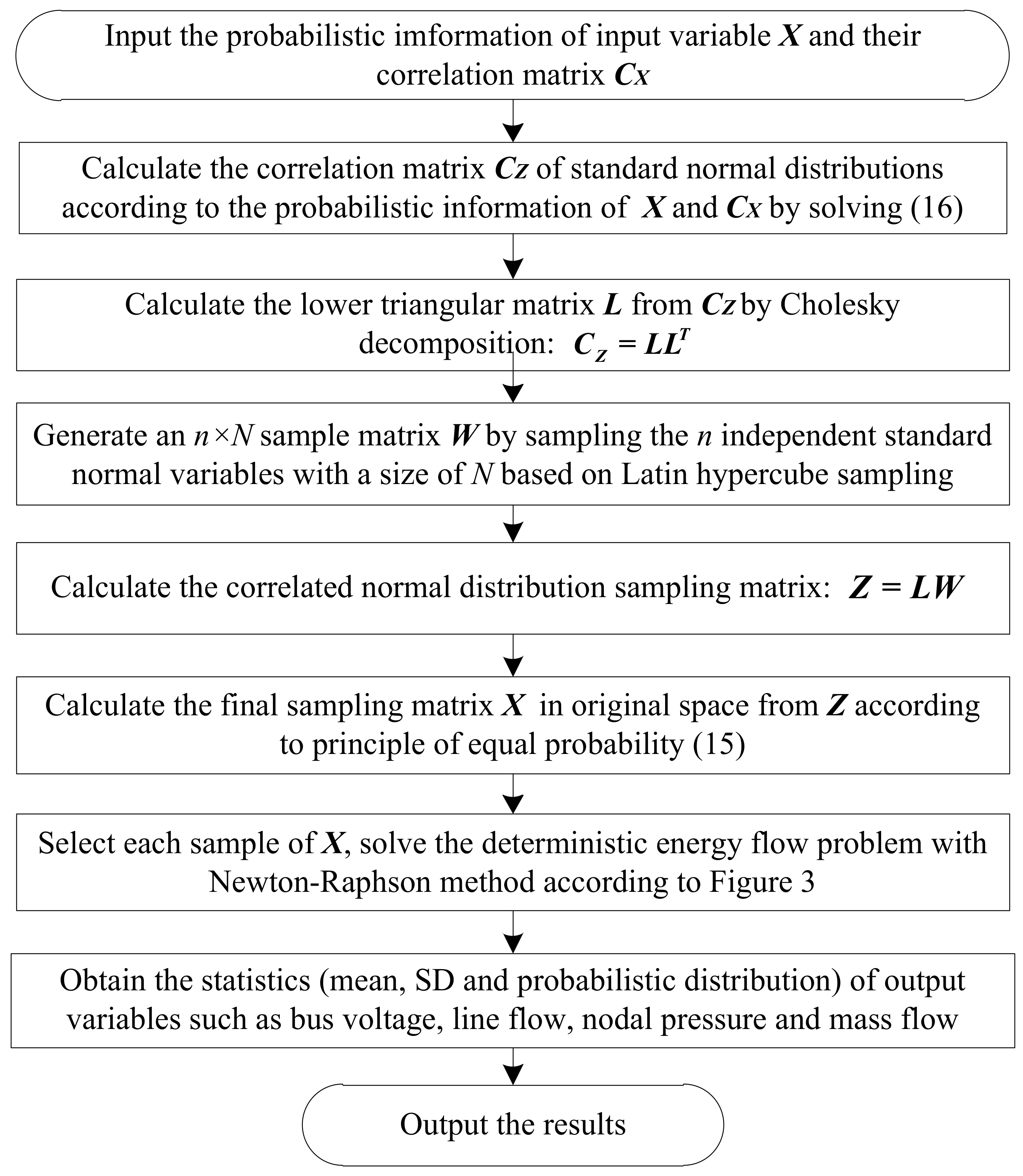
A PEF framework for an EGH-IES is proposed to address uncertainties and correlations in wind speed, photovoltaic power and electricity/gas/heat loads. A MCS method based on Latin hypercube sampling (LHS) and Nataf transformation (MCS-LN), which is able to accurately address correlated random variables following arbitrary distributions and effectively alleviate the computational burden of MCS, is then developed to solve the PEF problem.

(3)

Taking the operation mode “electricity/gas following heat” as an example, probabilistic interactions among the electricity/gas/heating networks and effects of uncertainties on the operation of the EGH-IES are investigated and discussed with numerical simulations.

The rest of this paper is organized as follows. Section 2 describes the steady-state modeling of the EGH-IES. Section 3 presents four typical operation modes of the EGH-IES. Section 4 presents the deterministic analysis of the EGH-IES. The probabilistic energy flow problem of an EGH-IES is formulated and then solved by the MCS-LN method in Section 5. Numerical results from a sample EGH-IES are presented and discussed in Section 6, and conclusions are finally given in Section 7.

2. Steady-State Modeling of the Electricity-Gas-Heat IES

2.1. Electricity Network

The typical AC power flow equations utilized for modeling an electricity network [20] can be expressed by

$$P_{\mathrm{G}i}-P_{\mathrm{L}i}=V_i{\displaystyle \sum _{j=1}^N{V}_j}\left(G_{ij}\cos {\delta }_{ij}+B_{ij}\sin {\delta }_{ij}\right)$$

(1)

$$Q_{\mathrm{G}i}-Q_{\mathrm{L}i}=V_i{\displaystyle \sum _{j=1}^N{V}_j}\left(G_{ij}\sin {\delta }_{ij}-B_{ij}\cos {\delta }_{ij}\right)$$

(2)

where P_Gi and Q_Gi are the active and reactive generation power at bus i (pu); P_Li and Q_Li are the active and reactive load power at bus i (pu); V_i (pu) and δ_i (rad) are the magnitude and angle of the voltage at bus i, and δ_ij = δ_i − δ_j; G_ij and B_ij are the real and imaginary parts of the element in the bus admittance matrix (pu); and N_b is the number of buses in the electricity network.

2.2. Natural Gas Network

A natural gas network usually consists of gas sources, pipelines, compressors and gas loads. The steady-state model of the natural gas network is described by the gas pipeline flow equations, compressor power equations and nodal gas flow balance equations [6].

Pipeline modeling is determined by its pressure rating. The pipeline equations applied to low pressure networks (0~75 mbar), medium pressure networks (0.75~7.0 bar) and high pressure networks (above 7.0 bar) are respectively expressed by [7]

$$F_{\mathrm{p},ij}=\{\begin{array}{l}5.72\times {10}^{-4}\sqrt{\frac{\left(p_i-p_j\right)D^5}{fL{S}_{\mathrm{G}}}}\\ 7.57\times {10}^{-4}\frac{T_n}{p_n}\sqrt{\frac{\left(p_i^2-p_j^2\right)D^5}{fLT{S}_{\mathrm{G}}}}\\ 7.57\times {10}^{-4}\frac{T_n}{p_n}\sqrt{\frac{\left(p_i^2-p_j^2\right)D^5}{fLTZ{S}_{\mathrm{G}}}}\end{array}$$

(3)

where F_p,ij is the gas flowing from node i to node j within pipeline p (m³/h); p_i and p_j are the pressures of node i and node j (mbar); T_n and p_n are respectively the temperature and pressure under standard conditions; f is the friction factor; L and D are the length and diameter, respectively, of pipeline p (m); T is the temperature of gas (°C); Z is the compressibility factor of gas; S_G is the specific gravity of gas.

Compressors are facilities installed in the natural gas network to compensate the pressure losses during gas transmission and thus to meet the pressure requirements of gas loads. Compressors can be driven by gas turbines or electricity turbines [23]. In the case of being driven by gas turbine, a compressor can be modeled as

$$\{\begin{array}{l}{H}_{\mathrm{c},ij}=B_{\mathrm{c}}{F}_{\mathrm{c},ij}\left({\left(\frac{p_j}{p_i}\right)}^{Z_{\mathrm{c}}}-1\right)\\ {\tau }_{\mathrm{c},ij}={\alpha }_{\mathrm{c}}+{\beta }_{\mathrm{c}}{H}_{\mathrm{c},ij}+{\gamma }_{\mathrm{c}}{H}_{\mathrm{c},ij}^2\end{array}$$

(4)

where H_c,_ij is the power consumed by the compressor connected to node i and j (horse power); F_c,_ij is the gas flowing through the compressor (m³/h); B_c is the parameter of the compressor relating to compressor efficiency, specific heat ratio of gas, gas compressibility and compressor temperature; Z_c is the parameter of the compressor relating to specific heat ratio of gas; τ_c,_ij is the amount of gas consumed by the compressor (m³/h); α_c, β_c and γ_c are consumption coefficients of the compressor.

As for the electricity-driven compressor, the relation between the power consumed and supplied is [20]

$$\{\begin{array}{l}{H}_{\mathrm{c},ij}=B_{\mathrm{c}}{F}_{\mathrm{c},ij}\left({\left(\frac{p_j}{p_i}\right)}^{Z_{\mathrm{c}}}-1\right)\\ P_{\mathrm{c},ij}=\frac{0.7457}{1000}{H}_{\mathrm{c},ij}\end{array}$$

(5)

where P_c,_ij is the electrical power supplied by the electricity network to the compressor (MW).

The gas flow balance equations at node i can be expressed by

$$F_i={\displaystyle \sum _{j\in i}{F}_{\mathrm{p},ij}}+{\displaystyle \sum _{j\in i}{s}_{\mathrm{c},ij}{F}_{\mathrm{c},ij}}+{\displaystyle \sum _{j\in i}{\tau }_{\mathrm{c},ij}}$$

(6)

where F_i is the injected gas flow at node i; $j\in i$ is the set of nodes connected to node i; s_c,ij = 1 if the inlet of the compressor is at node i; otherwise, s_c,ij = −1.

2.3. District Heating Network

The steady-state model of a district heating network consists of a hydraulic model and a thermal model. The hydraulic model [9] can be expressed by

$$\begin{array}{l}\mathit{A}\mathit{m}={\mathit{m}}_{\mathrm{q}}\\ \mathit{B}{\mathit{h}}_{\mathrm{f}}=\mathbf{0}\\ {\mathit{h}}_{\mathrm{f}}=\mathit{K}\mathit{m}\left|\mathit{m}\right|\end{array}$$

(7)

where A is the node-branch incidence matrix; m and m_q are, respectively, vectors of mass flow rate within each pipe and the injected mass flow at the nodes (kg/s); B is the loop-branch incidence matrix; h_f is the vector of head losses (m), and K is the vector of resistance coefficient of pipes.

With the thermal model, the heat power can be calculated by

$$\mathit{\Phi }=C_{\mathrm{p}}{\mathit{m}}_{\mathrm{q}}\left({\mathit{T}}_{\mathrm{s}}-{\mathit{T}}_{\mathrm{o}}\right)$$

(8)

where Φ is the vector of the heat power consumed or supplied (MW); C_p is the specific heat of water, C_p = 4.182 × 10⁻³ MJkg⁻¹ °C⁻¹; T_s is the vector of supply temperatures at nodes (°C); and T_o is the vector of the outlet temperature of flow at the outlet of nodes before mixing in the return network (°C).

The temperature relationship between the start and the end of pipe can be expressed [10] as

$$T_{\mathrm{end}}=e^{-\frac{{\lambda }_{\mathrm{t}}{L}_{\mathrm{t}}}{C_{\mathrm{p}}m}}\left(T_{\mathrm{start}}-T_{\mathrm{a}}\right)+T_{\mathrm{a}}$$

(9)

where T_start and T_end are temperatures at the start node and end node of the pipe, respectively (°C); λ_t is the total heat transfer coefficient per unit length; L_t is the length of the pipe (m); and T_a is ambient temperature (°C).

The mass flow mixing process is expressed as

$$\left({\displaystyle \sum m_{\mathrm{out}}}\right)T_{\mathrm{out}}={\displaystyle \sum m_{\mathrm{in}}{T}_{\mathrm{in}}}$$

(10)

where m_out and m_in are, respectively, the mass flow rate leaving and entering the node (kg/s); T_out is the mixture temperature at the node (°C); and T_in is the temperature of mass flow entering the mixing node at the end of the incoming pipe (°C).

2.4. Coupling Equipment

CHP unit, P2G and P2H facilities are considered in this paper. Note that the electricity-driven compressor is also a particular kind of coupling equipment, since it inputs power from the electricity network and outputs power to the gas network.

There are several kinds of CHP units (e.g., gas turbine CHP, reciprocating engine CHP and extraction steam turbine CHP). A gas turbine CHP unit, which produces electricity and heat power simultaneously by gas consumption, is considered in this paper. The model of a gas turbine CHP unit can be expressed as [13]

$$\begin{array}{l}{\Phi }_{\mathrm{CHP}}=c_{\mathrm{HP}}{P}_{\mathrm{CHP}}\\ F_{\mathrm{CHP}}=\frac{P_{\mathrm{CHP}}}{c_{\mathrm{GP}}}\end{array}$$

(11)

where Φ_CHP and P_CHP are the heat power and electrical power generated by the CHP unit; F_CHP is the gas consumed by the CHP unit; c_HP and c_GP are the heat-to-power ratio and gas-to-power ratio of the CHP unit, respectively.

P2G can convert electrical energy (usually excess renewable energy) to produce hydrogen, which is injected to the gas network or converted to synthetic natural gas. The simplified energy conversion relationship P2G can be found in [6]

$$F_{\mathrm{P}2\mathrm{G}}=C_{\mathrm{P}2\mathrm{G}}{P}_{\mathrm{P}2\mathrm{G}}$$

(12)

where P_P2G (MW) and F_P2G (m³/h) are, respectively, the electrical power consumed and the gas generated by the P2G; C_P2G is energy conversion coefficient of the P2G.

P2H equipment, such as electrical boilers and heat pumps, can convert excess renewable energy to heat. This paper considers electrical boilers, and the electricity-heat conversion relationship of P2H is

$${\Phi }_{\mathrm{P}2\mathrm{H}}={\eta }_{\mathrm{P}2\mathrm{H}}{P}_{\mathrm{P}2\mathrm{H}}$$

(13)

where Φ_P2H and P_P2H are, respectively, the heat power generated and electrical power consumed by the P2H (MW); and η_P2H is the energy conversion efficiency, η_P2H = 98% [24].

It is worth mentioning that both P2G and P2H provide promising prospects for accommodating renewable energy.

3. Operation Modes of the Electricity-Gas-Heat IES

The EGH-IES studied in this paper includes three subnetworks (i.e., electricity network, natural gas network and district heating network) and four kinds of coupling equipment (i.e., CHP unit, P2G, P2H and electricity-driven compressor), as shown in Figure 1.

According to the energy conversion relationships of the various pieces of coupling equipment and the power balances of each subnetwork, four typical operation modes of the EGH-IES (i.e., “electricity following heat” mode, “electricity/gas following heat” mode, “gas/heat following electricity” mode and “electricity following gas” mode) are suggested in this paper and depicted in Figure 2.

• Mode 1: “Electricity following heat” mode

As shown in Figure 2, when the EGH-IES works in mode 1, the heat node (i.e., the node in the heating network) connected to the P2H is set as the heat slack node and the P2H will maintain the overall heat power balance of the heating network. Therefore, variations in the heating network caused by such as variations in heat loads will change the heat power supplied by the P2H and then be transmitted to the electricity network via the P2H coupling. That is to say, the operation state of the electricity network in this mode will vary according to that of the heating network, or, in other words, variations in the heating network are followed by those of the electricity network. Note that, in this mode, the variation transmission between the electricity and heating network is single-directional and there is no reverse variation transmission from the electricity network to the heating network.

Moreover, when the EGH-IES works in mode 1, both the CHP and P2G are working with constant inputs/outputs and variations in one subnetwork will not be transmitted to the other via CHP or P2G. That is to say, there is no variation transmission between the gas and heating networks or between the electricity and gas networks provided that all compressors are gas-driven.

It should be noted that if there is even one electricity-driven compressor in the EGH-IES, there will be a variation transmission from the gas network to the electricity network. This is because the electrical power consumed by an electricity-driven compressor is determined by its pressure ratio and gas flow (see Equations (4) and (5)). This variation transmission is also single-directional (i.e., from the gas network to the electricity network) and can be found in all the four typical operation modes presented in this paper. Description of variation transmission from the gas network to the electricity network caused by electricity-driven compressor will not be repeated for the following three operation modes.

• Mode 2: “Electricity/gas following heat” mode

As also shown in Figure 2, when the EGH-IES works in mode 2, the heat node connected to the CHP is set as the heat slack node and the CHP will maintain the overall heat power balance of the heating network. Both the electrical power generated and gas consumed by the CHP in mode 2 are determined by its heat demands, which indicates that heat service has a priority over electricity service, and variations in the heating network will be transmitted to both the electricity and gas networks. This will finally lead to a three-sided variation transmission; that is, the variation transmission from the heating network to the electricity network and the variation transmission from the heating network to the gas network.

In mode 2, both P2H and P2G are working with constant inputs/outputs, and there is no variation transmission between the electricity and heating networks via P2H coupling or between the electricity and gas networks via P2G coupling.

• Mode 3: “Gas/heat following electricity” mode

When the EGH-IES works in mode 3, the electrical bus connected to the CHP is chosen as the electrical slack bus, and now the CPH will maintain the power balance of the electricity network, which is different from in mode 2. In this mode, the heat generated and gas consumed by the CHP is determined by its electricity demand, which also results in a three-sided variation transmission, but with different transmission directions, i.e., from the electricity network to the heating network, and from the electricity network to the gas network.

Similar to mode 2, both P2H and P2G in mode 3 are working with constant inputs/outputs, and they will not cause variation transmission between the electricity and heating networks or between the electricity and gas networks.

• Mode 4: “Electricity following gas” mode

When the EGH-IES works in mode 4, the gas node connected to the P2G is chosen as the gas slack node and the P2G will maintain the overall gas flow balance of the gas network. Therefore, variations in the gas network will change the gas demand of the P2G and then the operation state of the electricity network, which results in a single-directional variation transmission from the gas network to the electricity network.

As mentioned above, the compressor may be the other cause of the variation transmission from the gas network to the electricity network if it is driven by electricity. Therefore, an electricity-driven compressor is working in an “electricity following gas” mode, in essense.

Moreover, in mode 4, both CHP and P2H are working with constant inputs/outputs, and there is no variation transmission between the gas and heating networks or between the electricity and heating networks.

4. Deterministic Analysis of the Electricity-Gas-Heat IES

Steady-state models of an EGH-IES (Equations (1)–(13)), together with the operation modes presented in Section 3, constitute the deterministic energy flow (DEF) problem of the EGH-IES, which can be effectively solved by the Newton-Raphson method. Solution strategies for solving this DEF problem can be divided into two groups: the integrated method and the decomposed method. The integrated method solves all of the DEF equations simultaneously based on a unified Jacobian matrix, while the decomposed method solves the decoupled equations of each subnetwork successively and can deal with the operation modes of the EGH-IES effectively. Therefore, the decomposed method is used in this paper to solve the DEF problem, and different solving sequences are introduced to deal with the subnetworks according to the operation modes. A flowchart of the decomposed method considering the four typical operation modes is shown in Figure 3.

As shown in Figure 3, when the EGH-IES working in mode 1, mode 2 or mode 4, the three subnetworks are solved sequentially, i.e., the subnetworks are solved one by one. Specifically, in mode 1 and mode 4, the heating and gas networks are solved first, and then the electricity network is solved based on the solved heating and gas networks, while in mode 2, the solving sequence is as follows: the heating network is solved first, then the gas network, and finally the electricity network. Note that in mode 1 and mode 4, the heating and gas networks can be solved in parallel.

However, the solving sequence of mode 3 is quite different from other modes. In mode 3, the gas and electricity networks are not solved sequentially, but alternately. This is because in this mode, the bus connected to the CHP acts as the electrical slack bus, which means that there is a variation transmission from the electricity network to the gas network; meanwhile, the electricity-driven compressor poses a reverse variation transmission from the gas network to the electricity network. Moreover, the error of P_c (i.e., the electrical power consumed by the compressor) between two iterations can be used as the convergence criteria of the alternate solution.

5. Probabilistic Analysis of the Electricity-Gas-Heat IES

When considering uncertainties in such electricity/gas/heat loads and renewable energy sources, the DEF problem of the EGH-IES becomes a PEF problem. Any output variable of the EGH-IES, such as bus voltage, line power, nodal pressure, gas flow within gas pipeline, mass flow rate within heat pipe or supply temperature of heat load, can be expressed by

$$y=f\left(\mathit{x}\right)$$

(14)

where x is a vector of random input variables (e.g., electricity/gas/heat loads, wind speed and solar power, etc.), and y is the output variable.

In this paper, uncertainties in wind speed, photovoltaic power and electricity/gas/heat loads are considered, and the most widely used distributions are adopted to model these uncertainties (i.e., Weibull distribution for wind speed [18], Beta distribution for photovoltaic power [20] and normal distributions for loads [20,21]). Correlations among these uncertainties are also considered in this paper and are represented by a correlation matrix.

Therefore, probabilistic analysis of an EGH-IES or the task of PEF problem (14) is to obtain the probabilistic characteristics (e.g., mean and standard deviation (SD)) and probabilistic distributions (e.g., probabilistic density function (PDF) and cumulative distribution function (CDF)) of any output variable from the given distributions of the correlated uncertain wind speed, photovoltaic power and electricity/gas/heat loads.

The PEF problem (14) can be solved by many methods, and the MCS-LN method is developed to solve it in this paper. The MCS-LN method is based on LHS, Nataf transformation and repetitive solving of the DEF problem, where LHS is used to improve the sampling efficiency of Monte Carlo simulation and Nataf transformation is used to deal with correlations between uncertainties, especially correlations between uncertainties following non-normal distributions.

Both the procedure and the flowchart of the MCS-LN method for solving PEF problem 14 shown in Figure 4 can be summarized as follows.

Step 1: Calculate the correlation matrix of a standard normal distribution vector from the given correlation matrix of input random vector with Nataf transformation.

Let x = [x₁, x₂, …, x_n]^T be the n-dimensional input random vector with correlation matrix C_X. By applying the inverse transformation method, the random vector x can be described by a standard normal distribution vector Z composed of Z_k (k = 1, 2, …, n) with a different correlation matrix C_Z.

$$x_k=F_k{}^{-1}\left(\Phi \left(Z_k\right)\right),k=1,2,\cdots ,n$$

(15)

where F_k is the CDF of x_k, and Φ(·) denotes the single-variable standard normal CDF of Z_k .

The principal problem of Nataf transformation is to obtain the correlation matrix C_Z in normal space from the known correlation matrix C_X of input random vector x. For i ≠ j, let ρ_Z,ij be the element in the ith row and the jth column of C_Z, and let ρ_X,ij be the element in the ith row and the jth column of C_X, the relationship between each pair of ρ_Z,ij and ρ_X,ij is

$${\rho }_{X,ij}=\frac{{\displaystyle {\int }_{-\infty }^{\infty }{\displaystyle {\int }_{-\infty }^{\infty }{F}_i^{-1}\left[\Phi \left(z_i\right)\right]F_j^{-1}\left[\Phi \left(z_j\right)\right]{\phi }_{Z,ij}\left(z_i,z_j,{\rho }_{Z,ij}\right)d{z}_{i}d{z}_j}}-{\mu }_i{\mu }_j}{{\sigma }_i{\sigma }_j}$$

(16)

where μ_i(μ_j) and σ_i(σ_j) are, respectively, the means and SDs of x_i(x_j); $\phi$(z_i, z_j, ρ_Z,ij) is the PDF of the bi-variate standard normal distribution. ρ_Z,ij can be obtained from ρ_X,ij by Gauss–Hermite quadrature tool; more details can be found in [25].

Step 2: Calculate the lower triangular matrix L by Cholesky decomposition of C_Z as

$${\mathit{C}}_{\mathit{Z}}=\mathit{L}{\mathit{L}}^T$$

(17)

Step 3: Generate samples of n-dimensional uncorrelated random variables following the standard normal distribution based on LHS technique to form an n × N sample matrix W, where N is the sample size.

Step 4: Calculate the sample matrix Z of correlated normal distribution variables by

$$\mathit{Z}=\mathit{L}\mathit{W}$$

(18)

It can be mathematically proved that the correlation matrix of Z is C_Z [18].

Step 5: Calculate the sample matrix X of the original input random variables from Z by (15).

Step 6: Select each column of X, which is a sample of x in (14), and solve the DEF problem of the EGH-IES according to the flowchart shown in Figure 3.

Step 7: Obtain the numerical characteristics and probability distributions of the output random variables of the EGH-IES, including bus voltages and line flows of the electricity network, nodal pressures and gas flows within gas pipelines of the gas network, and supply temperatures and mass flow rates within the heat pipes of the heating network.

6. Case Studies

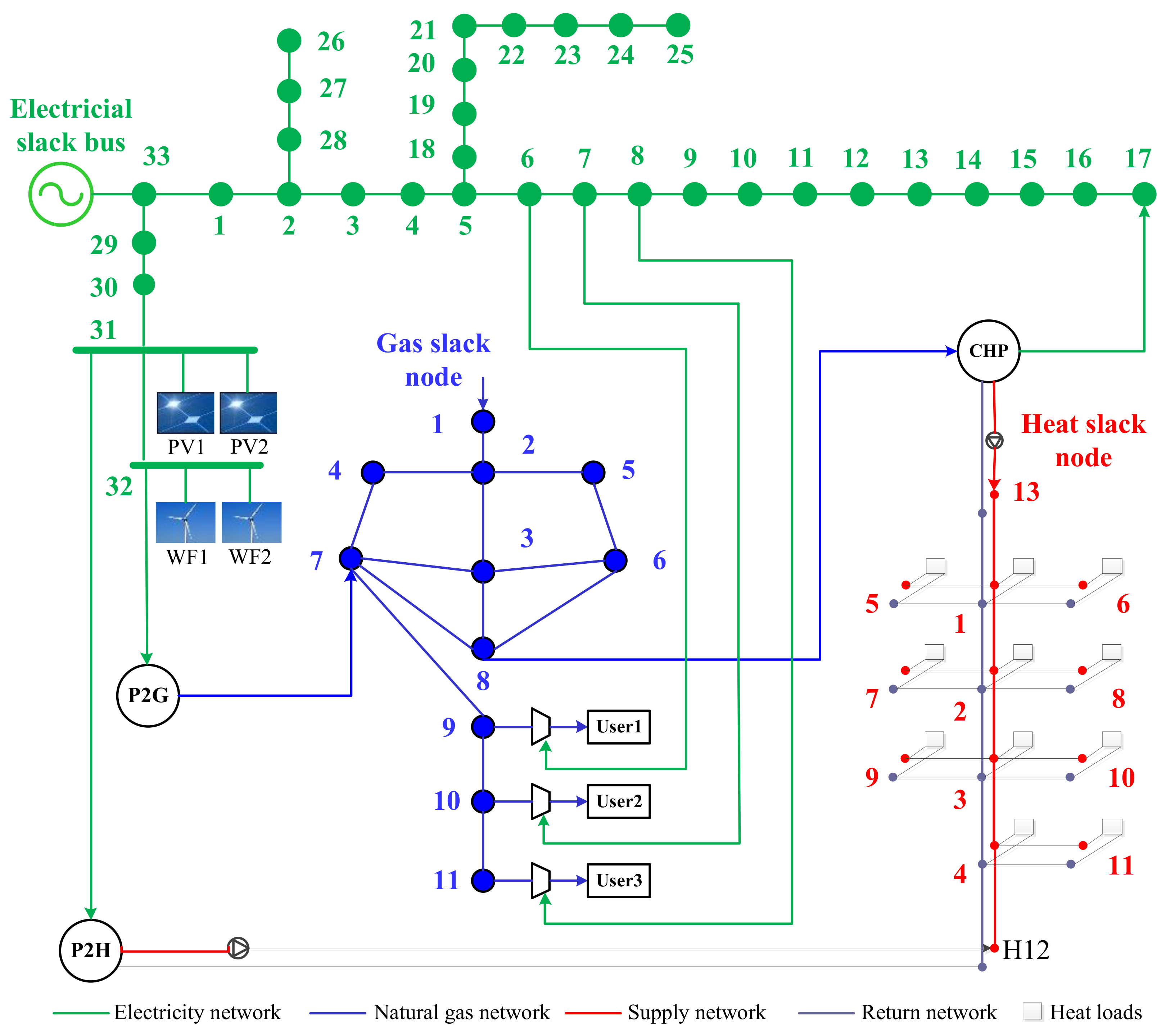
6.1. Test System Description

An EGH-IES composed of a 33-bus electricity network [26], an 11-node gas network [7] and a 13-node heating network [13] operating in the “electricity/gas following heat” mode is used as a test system to verify the proposed PEF analysis method. The configuration of the test system is shown in Figure 5. Although the case studies below are limited to the “electricity/gas following heat” mode, other operation modes can be studied in a similar way.

Two photovoltaic plants (PV1 and PV2) with a capacity of 0.75 MW each and unity power factors are connected to bus 31 in the electricity network. Active power of PV1 and PV2 are modeled by Beta distributions with shape parameters α₁ = β₁ = 0.9 and α₂ = β₂ = 0.95. There are also two wind farms (WF1 and WF2) in the electricity network. They are connected to bus 32 with a capacity of 0.5 MW each and power factors of 0.85 (lagging). Wind speeds are modeled by Weibull distributions. Parameters of the wind farms are listed in

Table 1. Parameters of the wind farms.

Wind Farm	Cut-in Speed (m/s)	Cut-out Speed (m/s)	Rated Speed (m/s)	Shape Parameter	Scale Parameter
WF 1	4	30	15	1.4	6.0
WF 2	5	28	14	1.8	6.8

.

The three subnetworks are coupled by a CHP unit connected to bus 17, gas node 8 and heat node 13, a P2H connected to bus 31 and heat node 12 and a P2G connected to bus 32 and gas node 7. In the 11-node gas network, gas node 1 connected to a gas source is chosen as the gas slack node and gas nodes 2~11 are all load nodes. The gas users (User 1, User 2 and User 3) shown in Figure 5 require a special pressure level of 37 mbar and therefore three electricity-driven compressors are installed to reach the required pressure level. In the 13-node heating network, heat node 13 connected to the CHP unit is the heat slack node and nodes 1~11 are all connected to heat loads.

All loads are modeled by normal distributions. The original electricity/gas/heat loads in Refs. [7,13,26] are taken as the mean values, and the SDs of loads are set to be 5% of their mean values.

6.2. Computational Performance of the MCS-LN Method

In this subsection, correlation coefficients among uncertainties are set as follows: ρ_EE = ρ_GG = ρ_HH = 0.5, ρ_WW = 0.6 and ρ_PP = 0.8, where the subscripts E, G, H, W and P denote electricity load, gas load, heat load, wind speed and photovoltaic power. Both λ_P2G and λ_P2H are set to be 0.1, where λ_P2G and λ_P2H denote the ratio of electrical power consumed by P2G and P2H to the total amount of power generated by wind farms and photovoltaic plants, respectively.

In order to test and validate the computational performance of the MCS-LN method, a similar method based on MCS with simple random sampling and Nataf transformation, denoted by MCS-SN, is also developed to solve the PEF problem. The PEF solution by the MCS-SN method with a sample size of 30,000 will be used as a reference for comparison.

The PEF results obtained by the MCS-LN method (with a sample size of 300) and the MCS-SN method (with a sample size of 30,000) are compared, and some results are given in

Table 2. Results of PEF for EGH-IES.

Indices	μloss	σloss	μF	σF	μT	σT
MCS-LN	0.3383	0.1027	30.0006	1.1139	98.8400	0.0450
MCS-SN	0.3377	0.0984	29.9975	1.1220	98.8400	0.0453
Relative error	0.17%	4.37%	0.01%	0.72%	0	0.66%

. The μ_loss and σ_loss are the mean value and SD of the active power loss of the electricity network. The μ_F and σ_F are the mean value and SD of the gas flowing through pipeline 10–11 (from node 10 to node 11). The μ_T and σ_T are the mean value and SD of the supply temperature at node 5 of the heating network, respectively. The relative errors are the errors in percentage between the two methods by taking the results obtained by the MCS-SN method as a reference.

As shown in Table 2, results obtained by the two methods are almost identical, and the largest relative error is less than 5%, which indicates that the MCS-LN method proposed can achieve high computational precision. In addition, the CPU time of the MCS-SN method and the MCS-LN method are, respectively, 41.85 s and 1285.92 s (both in a 2.5-GHz PC with a CPU of Inter(R) Core(TM) i7-6500U and 4G RAM), which highlights the computational efficiency of the MCS-LN method.

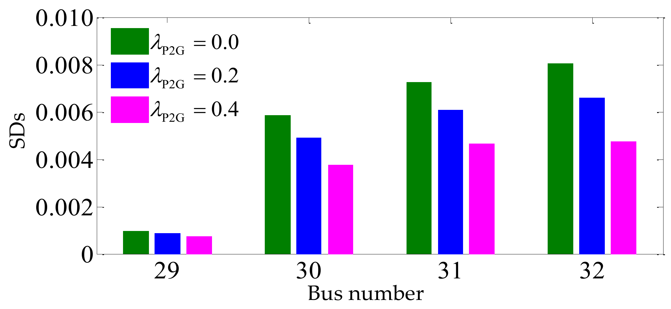
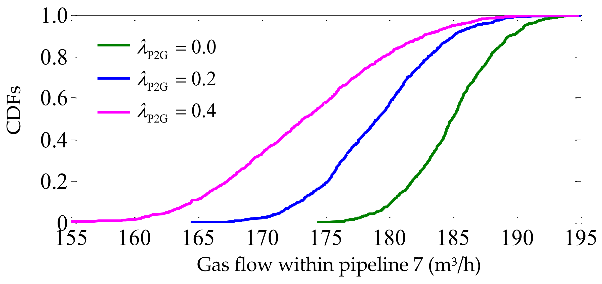
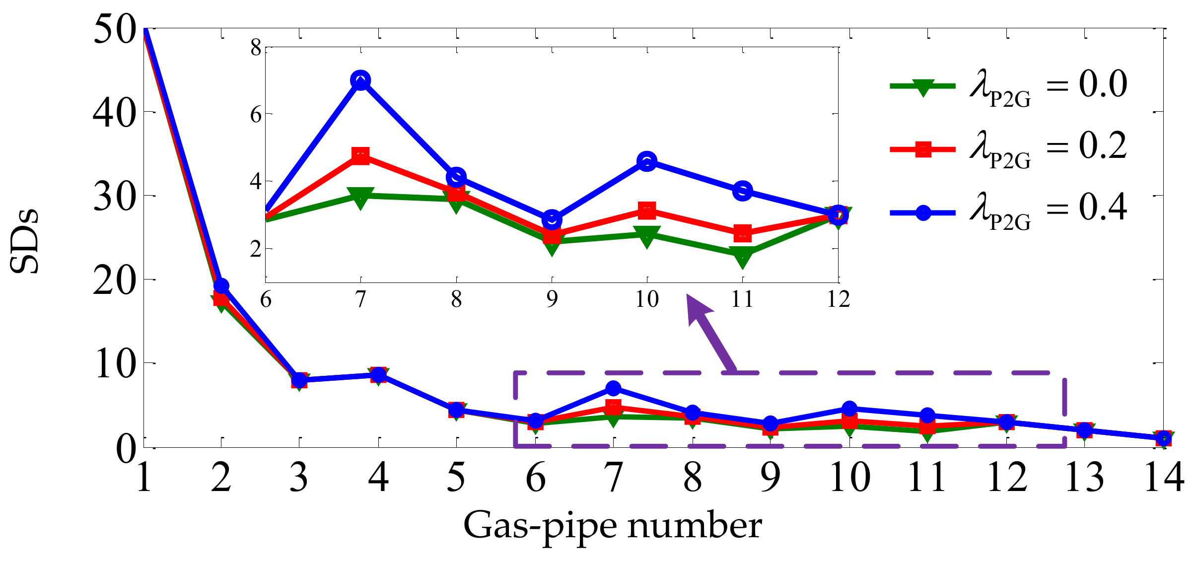
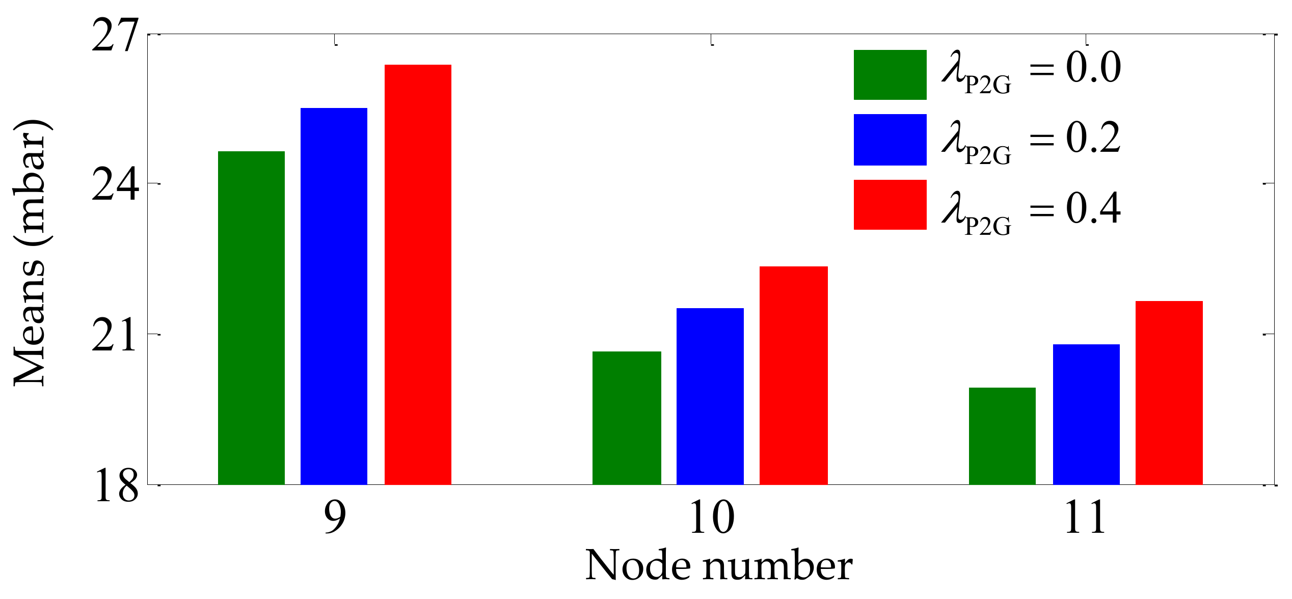
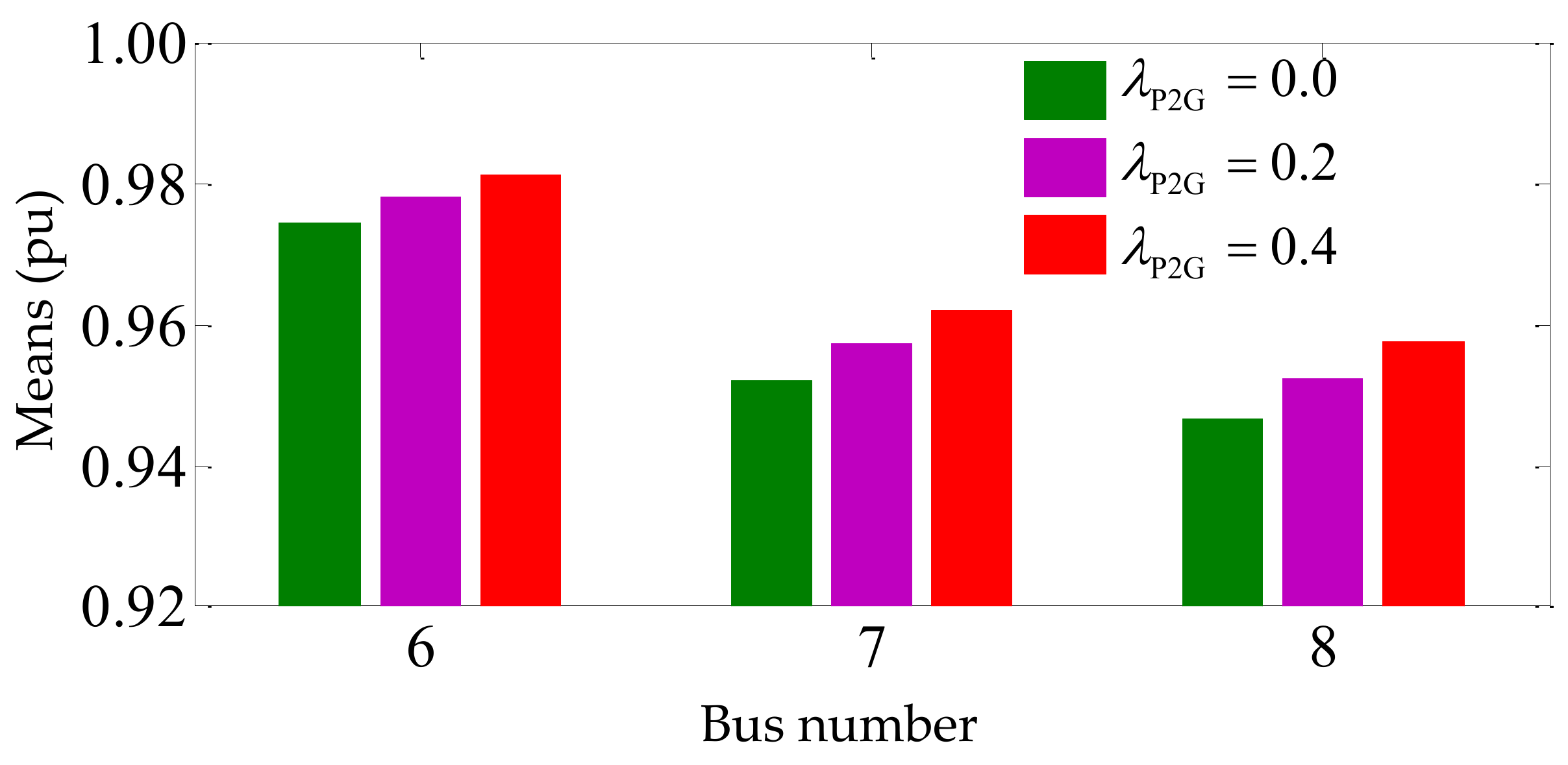
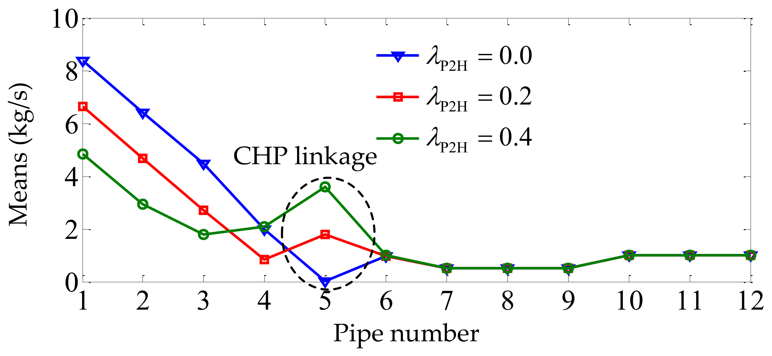
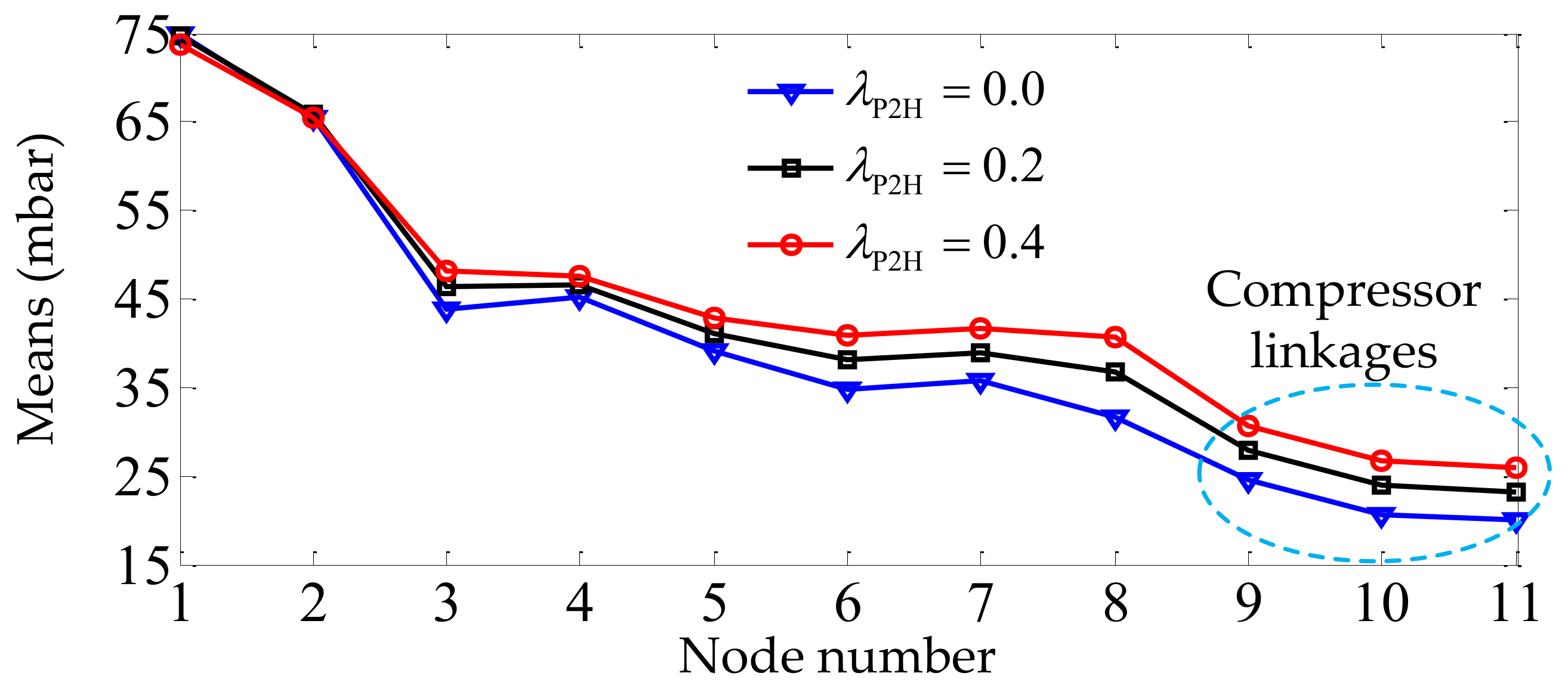
6.3. Effects of Different Conversion Levels of Electrical Power to Gas/Heat

Wind and solar power are typical intermittent renewable energy sources with high uncertainty. Under some special conditions, e.g., when high wind and/or solar power output and low electricity loads occur simultaneously, the surplus wind and/or solar power has to be curtailed to maintain the security of the electricity network. Clearly, this curtailment is undesirable and many efforts have been made to reduce or avoid it. As mentioned above, the utilization of both P2G and P2H provides a promising prospect for accommodating renewable energy.

In this subsection, we study the effects posed by the utilization of P2G and P2H on the operation of the EGH-IES and wind/solar power accommodation. Note that P2G/P2H are expected to convert wind and solar power to gas/heat in this paper, where they act as variable (or uncertain) electricity loads to the electricity network and variable (or uncertain) sources to the gas /heating networks and thus pose variable effects on the operation of the EGH-IES.

In order to study these variable effects, the PEF analysis proposed is conducted in this subsection with a focus on the effects of different conversion levels of electrical power to gas/heat (i.e., different λ_P2G and λ_P2H) on the operation of the EGH-IES. Accordingly, the following two cases are designed.

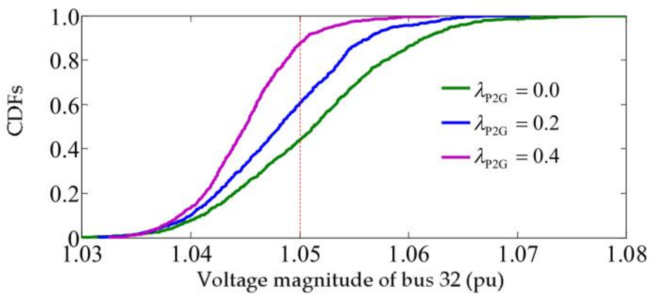
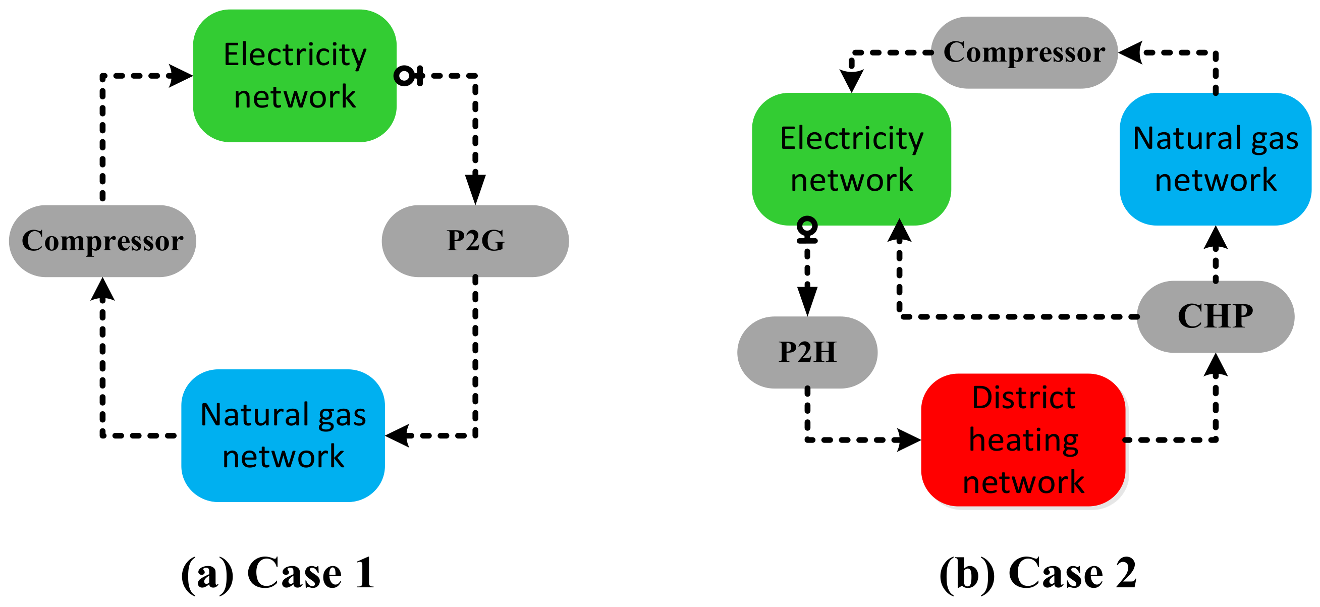
• Case 1: λ_P2G is set be 0, 0.2 and 0.4, while λ_P2H is kept at 0 (i.e., P2H is off).
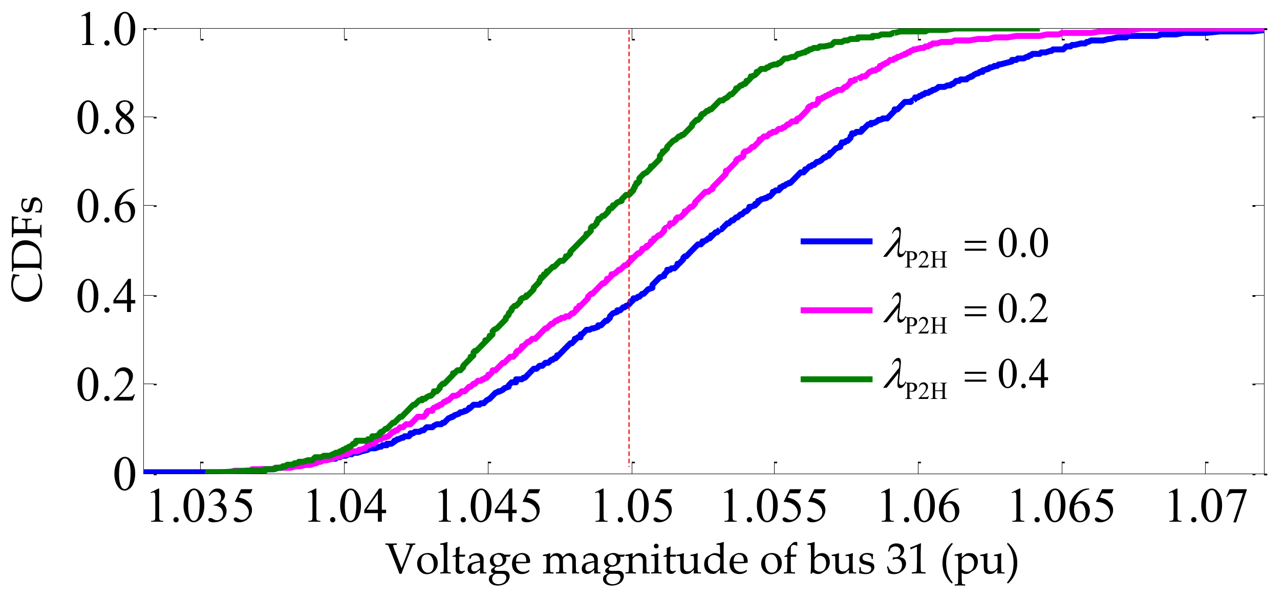
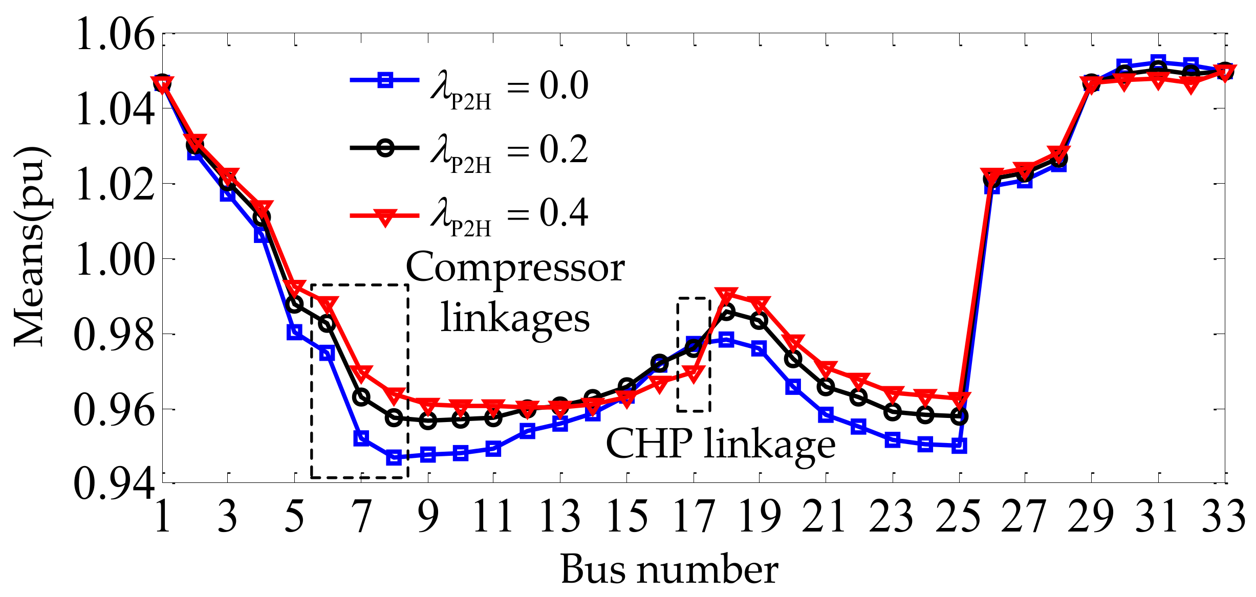
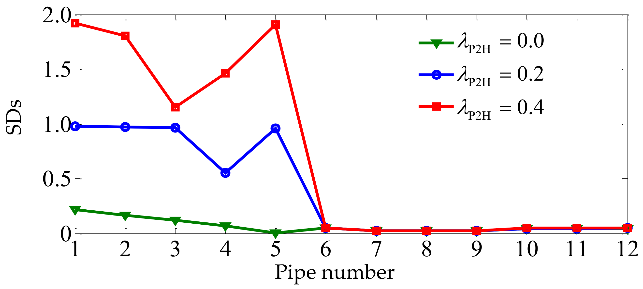
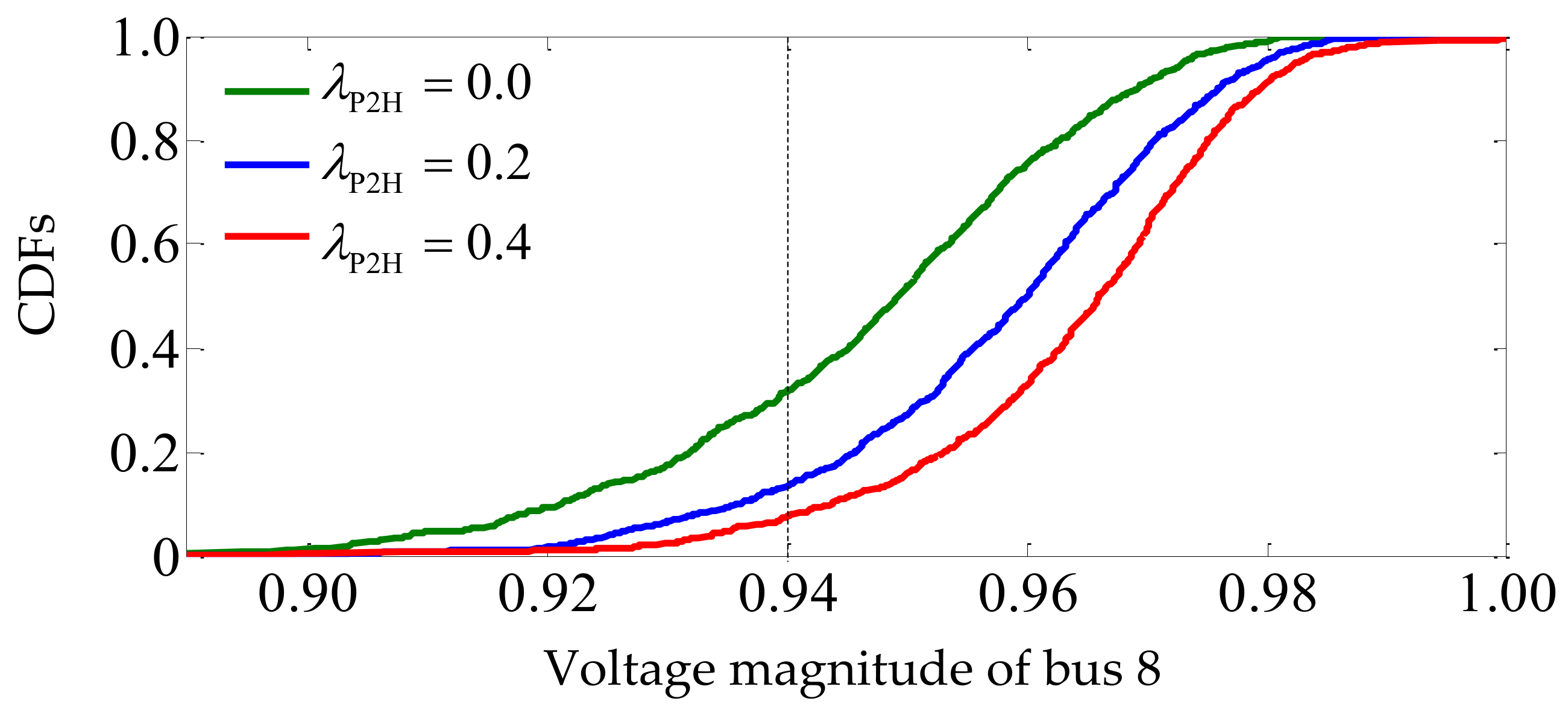
• Case 2: λ_P2H is set be 0, 0.2 and 0.4, while λ_P2G is kept at 0 (i.e., P2G is off).

Note that correlation coefficients among electricity/gas/heat load, wind speed and photovoltaic power are kept the same as those in the last subsection.

• Case 1

Figure 6 depicts the CDFs of voltage magnitude of bus 32, which is the bus connected to wind farms and P2G, and Figure 7 shows the SDs of voltage magnitudes of buses 29~32.

As shown in Figure 6, the CDFs of voltage magnitude of node 32 vary dramatically as λ_P2G changes. When P2G is off (λ_P2G = 0), the probability of the voltage magnitude at bus 32 exceeding its upper limit (set to be 1.05 pu) is up to 56.1%. However, this probability is dramatically reduced to 40% when λ_P2G = 0.2 and 12.6% when λ_P2G = 0.4. This indicates that the high wind and solar power output pose a high overvoltage threat to the electricity network, and the utilization of P2G can effectively alleviate this threat.

From Figure 7, it can be seen that the SDs of voltage magnitude of bus 32 (connected to wind farms), bus 31 (connected to solar plants) and bus 30 (close to bus 31) are much greater than that of bus 29. This indicates that buses 30~32 are affected greatly by the volatility of wind/solar power. It’s worth mentioning that as λ_P2G increases, there is a dramatic decrease in the SDs of voltage magnitude, especially at buses 30~32, which suggests that the utilization of P2G can also reduce the voltage fluctuation posed by the variable wind/solar power.

In addition to the voltages shown in Figure 6 and Figure 7, the output variables of the gas network are also investigated. The CDFs of gas flow within pipeline 7 (connected to gas nodes 3 and 8) and the SDs of gas flow within all pipelines are depicted in Figure 8 and Figure 9, respectively.

As shown in Figure 8, as λ_P2G increases, the gas flow within pipeline 7 tends to decrease, and thus the possibility of gas overloading also decreases. On the other hand, as λ_P2G increases, SDs of gas flow within pipeline 7 obviously increases (see Figure 9), and so does that of pipeline 10 (connected to gas nodes 6 and 8) and pipeline 11 (connected to nodes 7 and 8). These observations indicate that the utilization of P2G is helpful to reduce the overloading risk of the gas network, but may introduce harmful fluctuations resulted from uncertain wind/solar power to the gas flow especially within the pipeline directly connected to node 7 (to which the P2G is connected) and its nearby pipelines.

As mentioned above, there are three special gas users connected with nodes 7~9, and thus three electricity-driven compressors are installed to meet their pressure requirements. Figure 10 presents the mean values of the gas pressures of nodes 7~9 and Figure 11 gives further the mean values of voltages of the buses connected to the compressors.

As shown in Figure 10, the mean values of gas pressure of nodes 7~9 rise with the increase of λ_P2G, which indicates that the utilization of P2G is also helpful in improving the gas pressure of the end users. Additionally, it can be seen from Figure 11 that with the increase of λ_P2G, the voltages of buses 6~8 also increase. This is because the electrical power consumed by compressors decreases owing to the increased gas pressures (see (4) and (5)) and, accordingly, the voltages of the buses connected to the compressors improves.

• Case 2

Figure 12 depicts the CDFs of the voltage magnitude of bus 31 (connected to P2H) and Figure 13 gives the mean values of all voltage magnitudes in the electricity network. It can be seen that the utilization of P2H decreases the voltage level of bus 31 (see Figure 13), and thus the probability of bus 31 exceeding its upper voltage limit (see Figure 12), which is similar to the effect of P2G on the voltage of bus 32 in Case 1.

Figure 14 and Figure 15 present the mean values and SDs, respectively, of mass flow rates within pipes in the heating network. It can be observed from Figure 14 that as λ_P2H increases, the mass flow rates within some heavily loaded pipes (such as pipes 1~3) decrease remarkably, which indicates that P2H may contribute to reducing the potential overloading risks of the heating network. On the other hand, as λ_P2H increases, the SDs of mass flow rates within the main pipes (i.e., pipes 1~5) notably increases, because uncertainties in wind/solar power are introduced into the heating network via P2H. Note that the effects of P2H on overloading alleviation and SD increase are also similar to the effects of P2G on the gas network shown in Figure 8 and Figure 9 in Case 1.

However, different from Case 1, where P2G is the only uncertain gas source to the gas network, both P2H and CHP are uncertain heat sources for the heating network in Case 2, because the EGH-IES considered is working in the “electricity/gas following heat” mode. As mentioned above, in this mode, the CHP unit maintains the overall heat power balance of the heating network. Therefore, the uncertain output of the P2H due to uncertain wind/solar power will lead to uncertainty in the heat power generated by the CHP unit and finally impose uncertain impacts on both the electricity and gas networks. These uncertain impacts can be found in Figure 13, above, and Figure 16, shown below, which present the mean values of the gas pressures of all nodes in the gas network.

As shown in Figure 13, increasing λ_P2H leads to a voltage drop at bus 17 (connected to the CHP unit) and its nearby buses (i.e., buses 15 and 16). This is because with the output increase of the P2H, there is a decrease in the heat power output and correspondingly a decrease in the electrical power output of the CHP unit given that the overall heat loading level is unchanged, which finally results in a decrease in the voltages of bus 17 and its nearby buses.

From Figure 16, it can be seen that nodal pressures will increase with the increase of λ_P2H. This is because the amount of gas consumed by the CHP unit decreases due to its decreased heat and electrical power generation. This decreased gas consumption means a decrease in the overall gas loading level and therefore leads to an increase in nodal pressures.

Note that this pressure increment also leads to a decrease in the electrical power consumed by the compressors (see (4) and (5)), and therefore increases in the voltages of buses connected to compressors and their nearby buses (see Figure 13 for voltages of buses 5~9). Taking bus 8 as an example, CDFs of its voltage magnitude are shown in Figure 17. It can be observed from Figure 17 that as λ_P2H increases, the probability of voltage magnitude exceeding the lower limit (set to be 0.94 pu) decreases dramatically. This indicates that the utilization of P2H is helpful in improving the voltages not only of buses 30~32, connected to or near the wind farms and solar plants (see Figure 12 and Figure 13), but also the buses connected to the compressors.

• Comparison between Case 1 and Case 2

In this subsection, further comparative studies are performed on the uncertainty transmission among the subnetworks between Case 1 and Case 2, with an especial focus on the uncertainties originating from wind/solar power.

Figure 18 depicts the uncertainty transmission among the subnetworks, where the dashed arrows denote the transmission path of uncertainties, and the circles at the tail of the dashed line denote the uncertainties originated from the wind/solar power in the electricity network.

As shown in Figure 18a, in Case 1, uncertainties in the wind/solar power are transmitted to the gas network via P2G. These external uncertainties and the internal uncertainties in the gas loads make the operation states of the gas network more uncertain. On the other hand, uncertainties in the operation of the gas network, including the uncertainties from the external wind/solar powers, are transmitted back to the electricity network via electricity-driven compressor. Therefore, both electricity and gas networks suffer greater uncertainty because of the coupling between them by P2G and the electricity-driven compressor.

Note that in Case 1, the heating network is unaffected by the uncertainties in the wind/solar power because of the following facts: (a) the P2H is off in Case 1; (b) the EGH-IES is working in a “electricity/gas following heat” operation mode, where no uncertainty will transmit from the electricity network to the heating network.

As shown in Figure 18b, interactions among different subnetworks in Case 2 are more complicated than those in Case 1 because all three subnetworks are involved in Case 2. Uncertainties in wind/solar power are transmitted to the heating network via P2H. These uncertainties are further transmitted to the gas network and back to the electricity network through the CHP unit because of the role of the CHP unit in the “electricity/gas following heat” operation mode. Additionally, uncertainties in the gas network are also transmitted to the electricity network via the compressor, which is similar to Case 1. However, different from Case 1, uncertainties in wind/solar power in Case 2 are transmitted among all three subnetworks, including the heating network, and the operation uncertainty of all the three subnetworks, and thus the whole EGH-IES, is aggravated and complicated.

It is clear from the comparison above that the uncertain transmission among the subnetworks depends on the uncertainty sources, coupling equipment and their operation, and the operation mode of EGH-IES. However, given that there is coupling between any two subnetworks, the operation uncertainty of some (or all) subnetworks will be inevitably aggravated and complicated. This calls for probabilistic energy flow analysis to provide an accurate assessment of the operation of EGH-IES, thus motivating the studies in this paper.

6.4. Effects of Different Correlation Levels among Loads

The previous subsection studied the effects of different conversion levels of power to gas/heat on the operation of the EGH-IES and the corresponding uncertainty transmission among the subnetworks. In this subsection, we study further the effects of different correlation levels among uncertainty factors, especially the effects of different correlation levels among electricity, gas and heat loads. Effects of correlation levels between wind speeds and solar power, etc. can be studied in a similar way.

The following three testing scenarios with different correlation levels are considered:

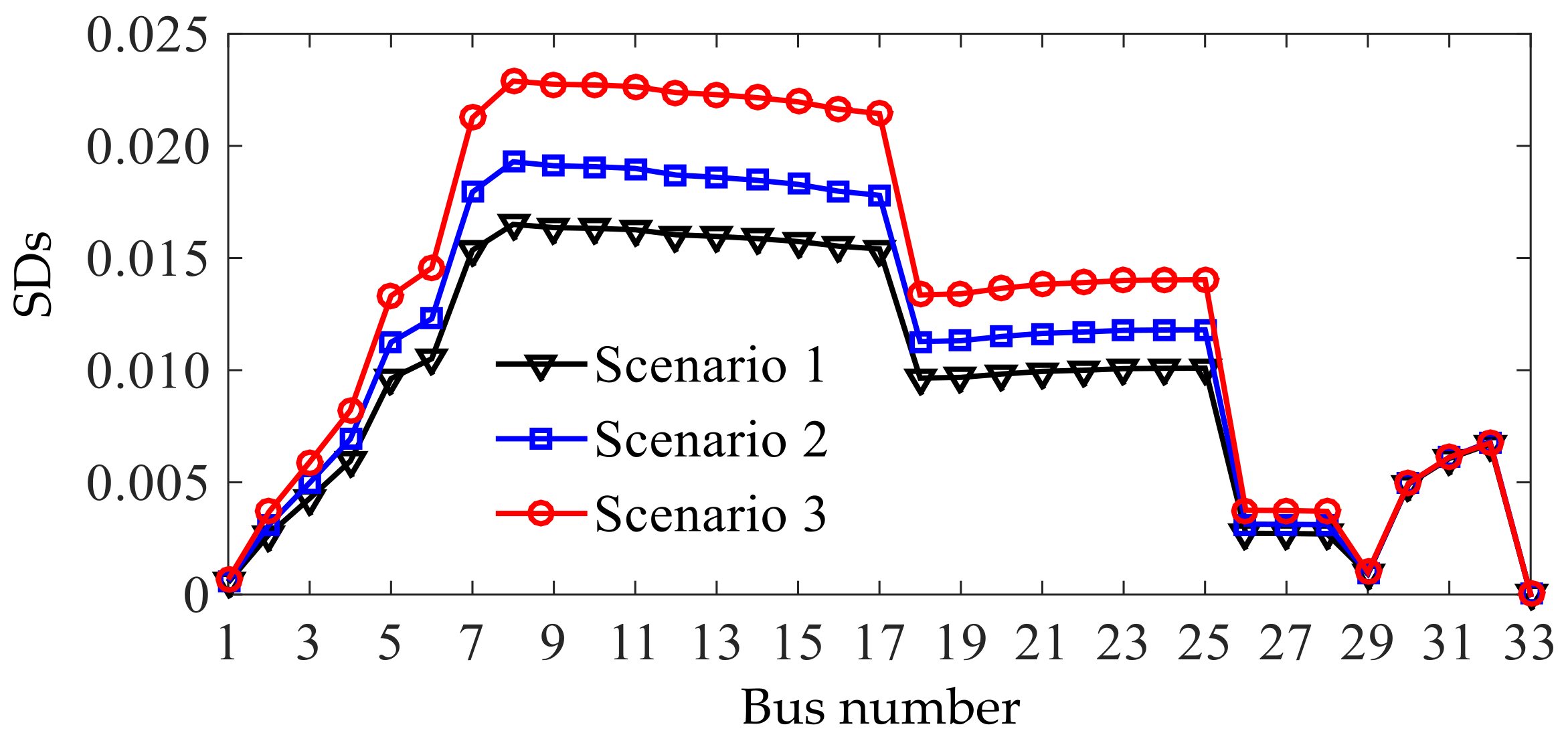
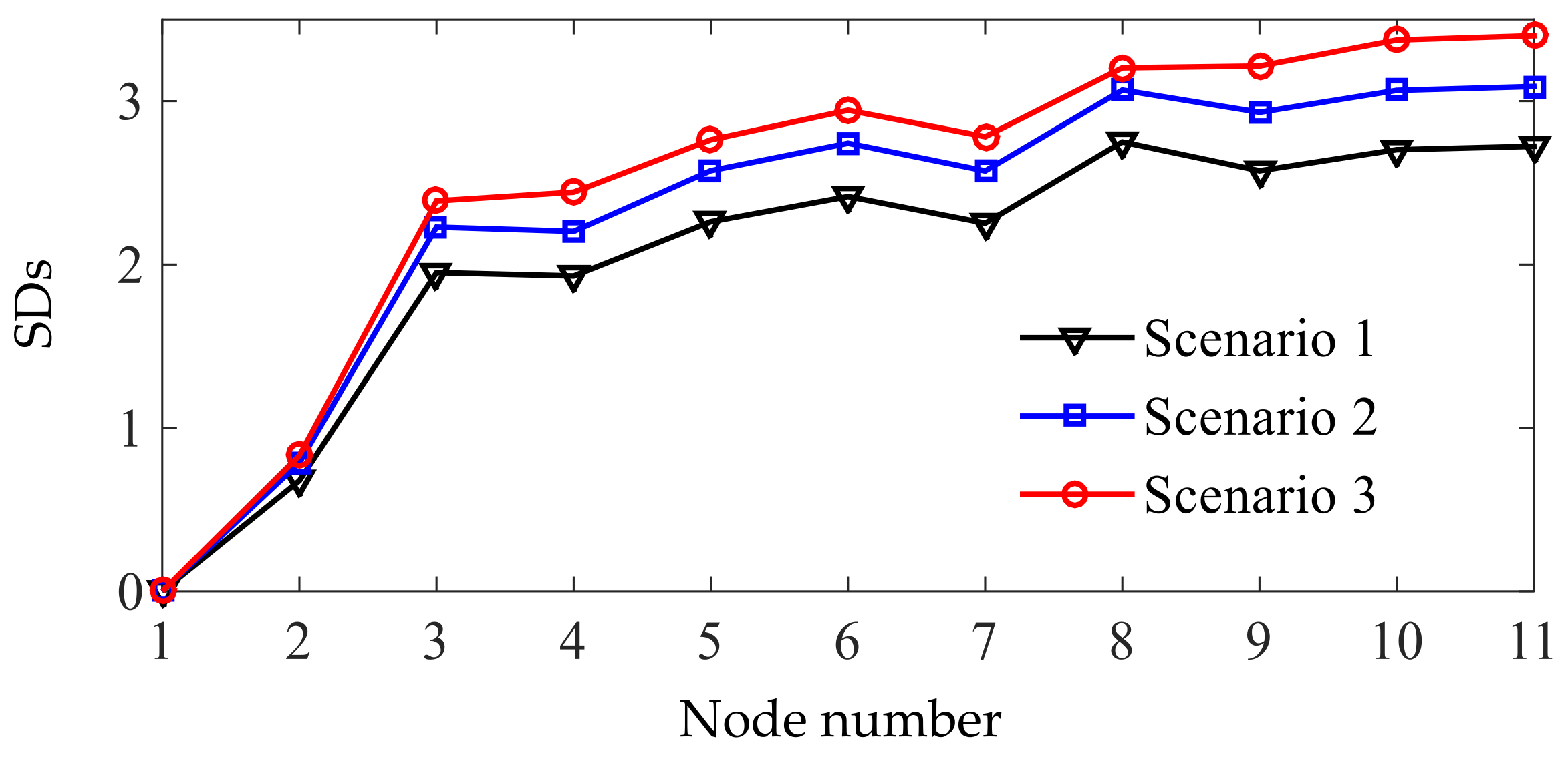
• Scenario 1: ρ_EG = ρ_EH = ρ_GE = 0;
• Scenario 2: ρ_EG = ρ_EH = 0.1, ρ_GH = 0.3;
• Scenario 3: ρ_EG = ρ_EH = 0.3, ρ_GH = 0.5.

Obviously, the loads are assumed to be uncorrelated in Scenario 1, and the correlation levels of Scenario 3 are higher than those of Scenario 2. Note that the other correlation coefficients (i.e., ρ_WW and ρ_PP) are the same as those in Section 6.2, and both λ_P2G and λ_P2H are set to be 0.1.

The PEF analysis proposed is conducted in this subsection to study the effects of correlation level on both the mean values and SDs of any output variable of the EGH-IES.

Simulation results indicate that different correlation levels among loads have negligible influences on the mean values and only some results related to the SDs (i.e., SDs of the voltage magnitudes and nodal pressures) are presented in Figure 19 and Figure 20 due to the limited space.

Figure 19 shows that the SDs of the voltage magnitudes at buses 1, 2, and 26~33 are slightly affected by variations in correlation of loads, while the SDs of other buses (especially buses 6~8 and 17) increase notably as the correlation levels increase from Scenario 1 to Scenario 3. This is because buses 1, 2, and 26~33 are near the slack bus (bus 33) of the electricity network, and buses 6~8 and 17 are the buses coupling to the gas and heating networks.

Similar observations can be made from Figure 20. In the gas network, the SDs of pressures of nodes 1 and 2 vary slightly and the SDs of other nodes increase notably from Scenario 1 to Scenario 3. The reason is that node 1 is the gas slack node and node 2 is close to node 1, which is similar to the explanation of Figure 19.

Theoretically, a greater correlation level among the electricity, gas and heat loads implies a higher possibility that electricity, gas, and heat loads increase or decrease simultaneously, which will lead to greater fluctuation in the energy flow of the EGH-IES. The simulation results shown in Figure 19 and Figure 20 verify this theoretical analysis. More importantly, the simulations presented above demonstrate the non-negligible effects of correlations on the operation of the EGH-IES and therefore the necessity of considering correlations in the PEF analysis.

7. Conclusions

This paper proposes a probabilistic steady-state analysis of an EGH-IES. Four typical operation modes of an EGH-IES (i.e., “electricity following heat” mode, “electricity/gas following heat” mode, “gas/heat following electricity” mode and “electricity following gas” mode) are presented at first. The probabilistic energy flow problem of the EGS-IES considering its operation modes and correlated uncertainties in the wind/solar power and electricity/gas/heat loads is then formulated and solved by the MCS method based on LHS and Nataf transformation. Finally, the probabilistic analysis proposed is tested and verified numerically on a sample EGH-IES working in the “electricity/gas following heat” mode.

Based on the simulation results, the following conclusions can be obtained:

(1)

The utilization of P2G/P2H has a double-edged effect on the operation of the EGH-IES. On the one hand, it is helpful in alleviating the overvoltage or overloading risks of the EGH-IES, but on the other hand, it may aggravate and complicate the uncertainty of the EGH-IES by transmitting uncertainties or variations in wind/solar power from the electricity network to the gas and heating networks.

(2)

Correlations among the electricity, gas and heat loads have non-negligible effects on the operation of the EGH-IES, and therefore they should be considered carefully in the PEF analysis of an EGH-IES.

(3)

Compared with existing studies on individual electricity, gas and heating systems, the electricity-gas IES, and electricity-heat IES, there are more complicated interactions and uncertainty transmissions among the subnetworks in an EGH-IES, which highlights the necessity of applying a probabilistic tool to the operation analysis of an EGH-IES.

(4)

The results obtained from the proposed probabilistic analysis framework for an EGS-IES can disclose the effects of uncertainties and interactions on the operation of EGH-IES, and thus provide an insight into the potential risks for the operators of EGH-IES. The results will also be a reference for the planning of EGH-IES.

References

- Clegg, S.; Mancarella, P. Integrated electrical and gas network flexibility assessment in low-carbon multi-energy systems. IEEE Trans. Sustain. Energy 2016, 7, 718–731. [Google Scholar] [CrossRef]
- Omalley, M.; Kroposki, B. Energy comes together: The integrated of all systems. IEEE Power Energy Mag. 2013, 11, 18–23. [Google Scholar] [CrossRef]
- Geidl, M.; Andersson, G. Optimal power flow of multiple energy carriers. IEEE Trans. Power Syst. 2007, 22, 145–155. [Google Scholar] [CrossRef]
- Krause, T.; Andersson, G.; Frohlich, K.; Vaccaro, A. Multiple-energy carriers: Modeling of production, delivery, and consumption. Proc. IEEE 2010, 99, 15–17. [Google Scholar] [CrossRef]
- Mancarella, P. MES (multi-energy systems): An overview of concepts and evaluation models. Energy 2014, 65, 1–7. [Google Scholar] [CrossRef]
- Zeng, Q.; Fang, J.K.; Li, J.H.; Chen, Z. Steady-state analysis of the integrated natural gas and electric power system with bi-directional energy conversion. Appl. Energy 2016, 184, 1483–1492. [Google Scholar] [CrossRef]
- Wang, W.L.; Wang, D.; Jia, H.J.; Chen, Z.Y.; Guo, B.Q.; Zhou, H.M.; Fang, M.W. Steady state analysis of electricity-gas regional integrated energy system with consideration of NGS networks status. Proc. CSEE 2017, 37, 1293–1304. [Google Scholar]
- Martinez-Mares, A.; Fuerte-Esquivel, C.R. A unified gas and power flow analysis in natural gas and electricity coupled networks. IEEE Trans. Power Syst. 2012, 27, 2156–2166. [Google Scholar] [CrossRef]
- Liu, X.Z. Combined Analysis of Electricity and Heat Networks. Ph.D. Thesis, Cardiff University, Wales, UK, 2013. [Google Scholar]
- Liu, X.Z.; Wu, J.Z.; Jenkins, N.; Bagdanavicius, A. Combined analysis of electricity and heat networks. Appl. Energy 2016, 162, 1238–1250. [Google Scholar] [CrossRef]
- Pan, Z.G.; Guo, Q.L.; Sun, H.B. Interactions of district electricity and heating systems considering time-scale characteristics based on quasi-steady multi-energy flow. Appl. Energy 2016, 167, 230–243. [Google Scholar] [CrossRef]
- Shabanpour-Haghighi, A.; Seifi, A.R. An integrated steady-state operation assessment of electrical, natural gas and district heating networks. IEEE Trans. Power Syst. 2016, 31, 3636–3647. [Google Scholar] [CrossRef]
- Wang, Y.R.; Zeng, B.; Guo, J.; Shi, J.Q.; Zhang, J.H. Multi-energy flow calculation method for integrated energy system containing electricity, heat and gas. Power Syst. Technol. 2016, 40, 2942–2950. [Google Scholar]
- Liu, X.Z.; Mancarella, P. Modelling, assessment and Sankey diagrams of integrated electricity-heat-gas networks in multi-vector district energy systems. Appl. Energy 2016, 167, 336–352. [Google Scholar] [CrossRef]
- Clegg, S.; Mancarella, P. Integrated electricity-heat-gas modelling and assessment, with applications to the Great Britain system. Part II: Transmission network analysis and low carbon technology and resilience case studies. Energy 2018. [Google Scholar] [CrossRef]
- Cascio, E.L.; Borelli, D.; Devia, F.; Schenone, C. Future distributed generation: An operational multi-objective optimization model for integrated small-scale urban electrical, thermal and gas grids. Energy Convers. Manag. 2017, 143, 348–359. [Google Scholar] [CrossRef]
- Shabanpour-Haghighi, A.; Seifi, A.R. Simultaneous integrated optimal energy flow of electricity, gas, and heat. Energy Convers. Manag. 2015, 101, 579–591. [Google Scholar] [CrossRef]
- Chen, Y.; Wen, J.Y.; Cheng, S.J. Probabilistic load flow method based on Nataf transformation and Latin hypercube sampling. IEEE Trans. Sustain. Energy. 2013, 4, 294–301. [Google Scholar] [CrossRef]
- Aien, M.; Fotuhi-Firuzabad, M.; Aminifar, F. Probabilistic load flow in correlated uncertain environment using unscented transformation. IEEE Trans. Power Syst. 2012, 27, 2233–2241. [Google Scholar] [CrossRef]
- Chen, S.; Wei, Z.N.; Sun, G.Q.; Wang, D.; Sun, Y.H.; Zang, H.X.; Zhu, Y. Probabilistic energy flow analysis in integrated electricity and natural-gas energy systems. Proc. CSEE 2015, 35, 6331–6340. [Google Scholar]
- Chen, S.; Wei, Z.N.; Sun, G.Q.; Cheung, K.W.; Sun, Y.H. Multi-linear probabilistic energy flow analysis of integrated electrical and natural-gas systems. IEEE Trans. Power Syst. 2017, 32, 1970–1979. [Google Scholar] [CrossRef]
- Hu, Y.; Lian, H.R.; Bie, Z.H.; Zhou, B.R. Unified probabilistic gas and power flow. J. Mod. Power Syst. Clean. Energy 2017, 5, 400–411. [Google Scholar] [CrossRef]
- Yang, L.; Zhao, X.; Hu, X.Y.; Sun, G.R.; Yan, W. Probabilistic power and gas flow analysis for electricity-gas coupled networks considering uncertainties in pipeline parameters. In In Proceedings of the 2017 IEEE Conference on Energy Internet and Energy System Integration (EI2), China, Beijing, 26–28 November 2017; pp. 1–6. [Google Scholar]
- Sun, J.; Wei, Z.N.; Sun, G.Q.; Chen, S.; Zang, H.Y.; Chen, S. Analysis of probabilistic energy flow for integrated electricity-heat energy system with P2H. Electr. Power Autom. Equip. 2017, 37, 62–68. [Google Scholar]
- Li, H.S.; Lü, Z.Z.; Yuan, X.K. Nataf transformation based point estimate method. Chin. Sci. Bull. 2008, 53, 2586–2592. [Google Scholar] [CrossRef]
- Liu, H.; Tang, C.; Han, J.; Li, T.; Li, J.F.; Zhang, K. Probabilistic load flow analysis of active distribution network adopting improved sequence operation methodology. IET Gener. Trans. Distrib. 2017, 11, 2147–2153. [Google Scholar] [CrossRef]