Flexible Biogas in Future Energy Systems—Sleeping Beauty for a Cheaper Power Generation

Abstract

The increasing proportion of intermittent renewable energies asks for further technologies for balancing demand and supply in the energy system. In contrast to other countries, Germany is characterized by a high installed capacity of dispatchable biogas plants. For this paper, we analyzed the total system costs varying biogas extension paths and modes of operation for the period of 2016–2035 by using a non-linear optimization model. We took variable costs of existing conventional power plants, as well as variable costs and capital investments in gas turbines, Li-ion batteries, and pumped-storage plants into account. Without the consideration of the costs for biogas plants, an increasing proportion of biogas plants, compared to their phase out, reduces the total system costs. Furthermore, their flexible power generation should be as flexible as possible. The lowest total system costs were calculated in an extension path with the highest rate of construction of new biogas plants. However, the highest marginal utility was assessed by a medium proportion of flexible biogas plants. In conclusion, biogas plants can be a cost-effective option to integrate intermittent renewable energies into the electricity system. The optimal extension path of biogas plants depends on the future installed capacities of conventional and renewable energies.

1. Introduction

The increasing greenhouse gas (GHG) emissions and the resulting negative impacts of climate change compel the international community to act. In December 2015, the Paris Agreement was signed to limit global warming to one and a half degree Celsius compared with preindustrial levels [1]. Worldwide, net zero carbon emissions has to be achieved by the middle of the 21st century [2]. By 2050, in order for Germany to reduce GHG emissions by at least 80% compared to 1990, the German government’s Energy Action Plan 2050, signed in 2016, aims to decrease total GHG emissions by 55–56% and the energy sector’s GHG emissions by 61–62% by 2030 [3]. The proportion of renewable energies in the electricity system is specified by the Renewable Energy Sources Act (EEG), by 2025 the proportion should make up 40–45% of gross electricity consumption and by 2035 55–60% [4]. According to the EEG, the future German electricity generation will be based on intermittent renewable energies, namely wind and photovoltaic plants [4]. Due to their intermittency of power generation, further technologies balance the demand and supply, such as demand-side management (DSM), grid extension, storage technologies, and supply-side flexibility, which can be used to integrate them into the energy system [5,6]. In contrast to other countries in Europe, in 2016 17.2% of Germany’s renewable electricity generation was generated by biogas plants [7], whereby these are the most important dispatchable renewable energy. As a consequence, flexible power generation from biogas plants can be one technical solution of low GHG emissions to integrate intermittent renewable energies into the electricity system [8,9,10]. Furthermore, compared to the use of biogas and biomethane (a natural gas substitute) for direct heating or transport in Germany, the highest GHG emission savings can be achieved by the generation of heat and electricity in combined heat and power units (CHPU) [11].

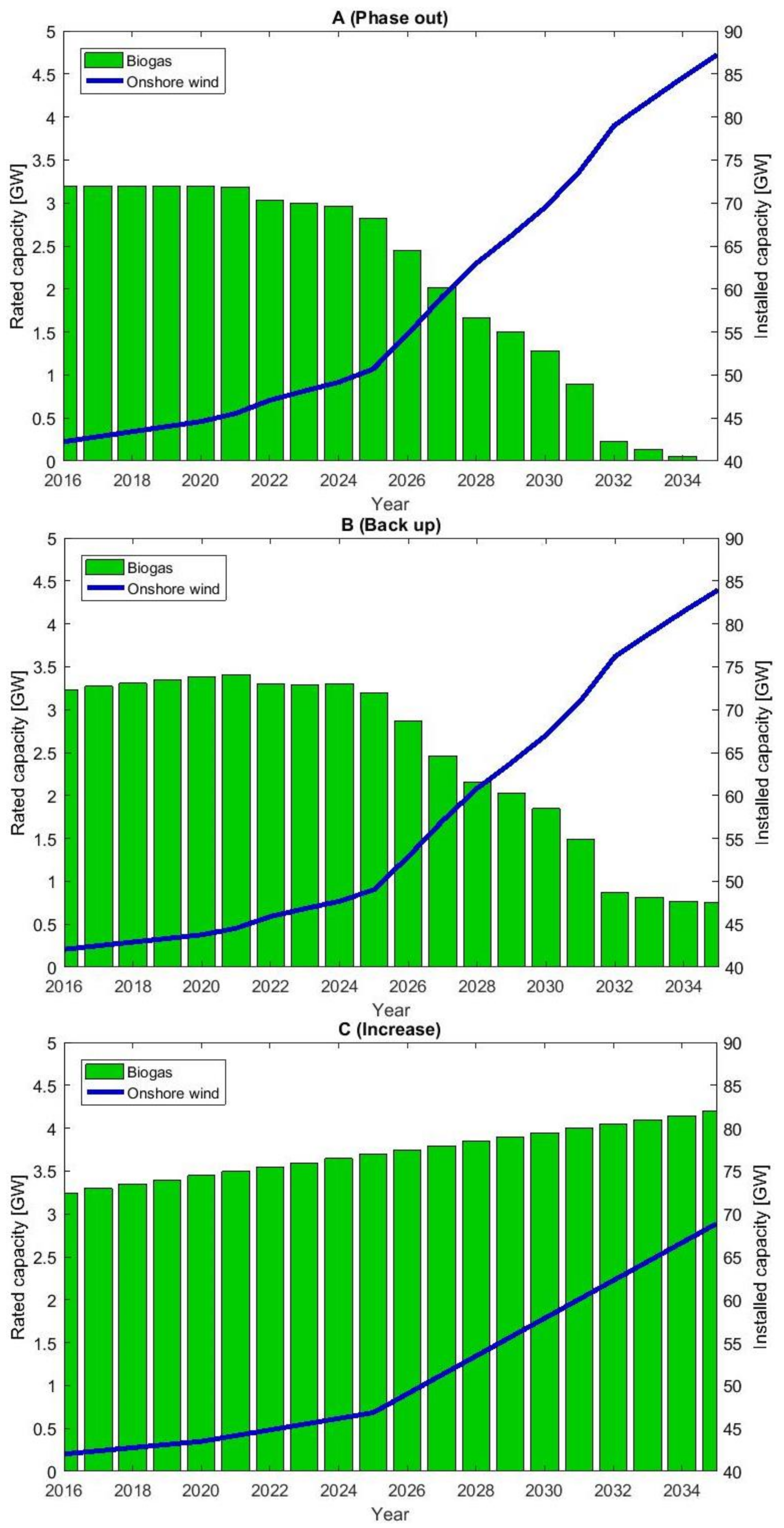
Nevertheless, in 2016, the German Government has decided to decrease the installed capacity and the electricity generated by biomass (and biogas) plants within the next decades. The EEG reform limits the annual expansion to a maximum of 150 MW (2017–2019) and 200 MW (2020–2022) [4]. Due to the average biogas plants installation of 350 MW per year in the period of 2004–2014 [12], fewer biogas plants will be built and those remaining will begin to close down after their 20 year periods of remuneration in the 2020s. As a result, the installed capacity of biomass, and especially biogas plants, will be reduced and other flexibility options will become more important to ensure there is a sufficient power supply based on intermittent renewable energies in the future German electricity system. If flexible power generation from biogas plants decreases, additional capacities of storage technologies and dispatchable (conventional) power plants might be needed that accompany enhancing investments. In this study, we calculate the total system costs in the future German electricity system depending on varying biogas extension paths.

The cost-effective transformation of the energy system towards decarbonization and an increasing proportion of renewable energies in the electricity, as well as in the heating and mobility sector, is a topic of a high number of publications in recent years. Urzúa et al. [13] showed the impact of an increasing proportion of intermittent renewable energies on the total system costs in Chile. Due to additional costs for transmission and renewable energy capacities, the total costs increase with further wind and solar plants. Due to this, the investments in coal-fired power plants and their base-load operation are cheaper than the combination of (intermittent) renewable energies and transmission grids. Therefore, they argue that dispatchable renewable energies, such as base-load generated hydropower or biomass, can be better integrated in the existing energy system of Chile. Jacobson et al. [14] analyzed the social cost of a 100% renewable US energy system by 2050–2055, including all sectors. Compared to a fossil system, they calculated that the power generation by wind, water, and solar is more economically feasible when the cost of health and climate are integrated. The cost of the electric system in a renewable energy system is about 11.37 ct∙kWh⁻¹, while, including the externality of conventional power generation, the cost of the electric system is given of 27.6 ct∙kWh⁻¹ in a non-renewable energy system. Budischak et al. [15] optimized the least-cost combinations of intermittent renewable energies and storage technologies in a large regional grid in the Eastern USA. The aim is to supply the demand in this area. They found that when 290% of the demand is generated by the optimal combination of renewable energies and storage technologies, 99.9% of the hourly demand over four years can be covered. Depending on the chosen storage technology only 9–72 full load hours of storage technologies are required to fulfill the target value. Furthermore, regarding the technology costs by 2030, the renewable energy electricity system will be more cost-effective than the conventional one today.

In Europe, similar studies regarding the transformation process of the energy system were also carried out. Heide et al. [16] calculated the optimal mix of photovoltaics (PV) and wind power plants in a fully-renewable European power system to minimize three different objectives: storage capacities, balancing energy, and balancing power. According to their results, depending on the objectives, three different optimal solutions were found. To minimize the storage requirements, the mix of 60% wind and 40% PV has to be chosen when ideal roundtrip storage is used. Nevertheless, they do not take economic analysis into account. Pfenninger and Keirstead [17] combined three technologies, namely renewables, nuclear, and fossil fuels used in Great Britain’s power system to reach different targets of CO₂ emissions reduction, energy security and system-wide levelized cost of electricity (LCOE). Their analysis showed that different combinations of the chosen technologies lead to similar results. From the perspective of renewables, a proportion of up to 80% relates to a significant increase of cost. However, a proportion above 80% asks for high investments in large-scale storage, imports of (renewable) power, or additional dispatchable renewables. Brouwer et al. [18] analyzed which flexibility options in the Western Europe power system should be used to minimize the total system costs 2050. These included demand response, natural gas-fired generators, interconnection capacity, curtailment of intermittent renewables, and electricity storage. With the exception of storage technologies, all flexibility options may reduce total system costs within varying proportions of renewable energies. Zakeri et al. [19] examined the technical and economic feasibility of flexibility options to integrate intermittent renewable energies in energy systems with a high proportion of non-flexible nuclear power generation. However, the role of biomass as a flexibility option and its impact on total system costs is not shown in detail, although, these plants are assumed as flexible as coal-fired power plants with carbon capture storage.

In Germany, based on a high proportion of biomass plants, several studies analyze their current and future role in the electricity system. Holzhammer [20] calculated that flexible power generation from biogas plants and biomethane CHPU might reduce total system costs in 2030. One reason is that it saved fuels and the lower numbers of start-stop operations, inter alia, by conventional power plants overcompensate additional costs for flexible power generation from biogas plants with a number of 4000 full load hours per year. In a previous study [21] we assessed the flexible biogas power generation using the average integration costs of surplus generation (AICSG) for the period of 2016–2035, which is defined as a quotient of remuneration and surplus generation. We find that biogas plants have to be as flexible as possible to smooth the future residual load curve and to reduce the further demand for flexibility options in Germany. Furthermore, the increasing extension of biogas plants may be more cost-effective for the system integration of intermittent renewable energies than their reduction or phase out. In another study for Germany, Eltrop et al. [22] calculated, endogenously, the installed capacities of lignite-, coal-, gas-fired power plants, biomass plants, and storage technologies using the European Electricity Market Model E2M2s. It is shown that varying the proportion of renewable energies (40%, 60%, and 80%) an endogenous extension of the installed capacity of flexible biomass plants can reduce the total electricity system costs. The annual amount of electricity generated by biomass plants is set to be constant. Due to saved investments in storage technologies and conventional power plants, regarding a proportion of 80% of renewable energies, flexible biomass plants reduce the total electricity system costs by 419 million € (compared to baseload generation).

To summarize, the above-mentioned studies show the impact of renewable energies on total system costs or the demand for further technologies to balance demand and supply, which become more important during the energy transformation process. The future role of flexible power generation from biomass plants is especially analyzed in German publications. Nevertheless, the impact of varying biogas extension paths exogenously by policy makers on the composition of flexibility options and the total costs in the future German electricity system is not taken into account in previous publications. In contrast to the endogenous optimization of flexibility options, e.g., in [18], the installed capacity of Germany’s biogas plants is set by the EEG based on the decision of the German Government. Furthermore, according to the EEG revised in 2016 [4], details of the flexible biogas power generation are given by policy makers. For example, the power quotient PQ [9] which is defined as the quotient of installed and rated capacity—the annual average of electricity generation—of biogas plants has to be 2 or higher (EEG 2017, § 44b). With regard to the transformation process of the energy system towards renewable energies, the future role of flexible power generation from biogas plants determined exogenously by policy makers has to be assessed. In addition to other flexibility options, biogas plants might be one cost-effective option to integrate intermittent renewable energies into Germany’s energy system.

In this paper, we assess the composition of flexibility options and the total costs in the German electricity system for the period of 2016–2035 by using a non-linear optimization model varying the extension path and mode of operation of biogas plants.

The objectives can be defined as follows:

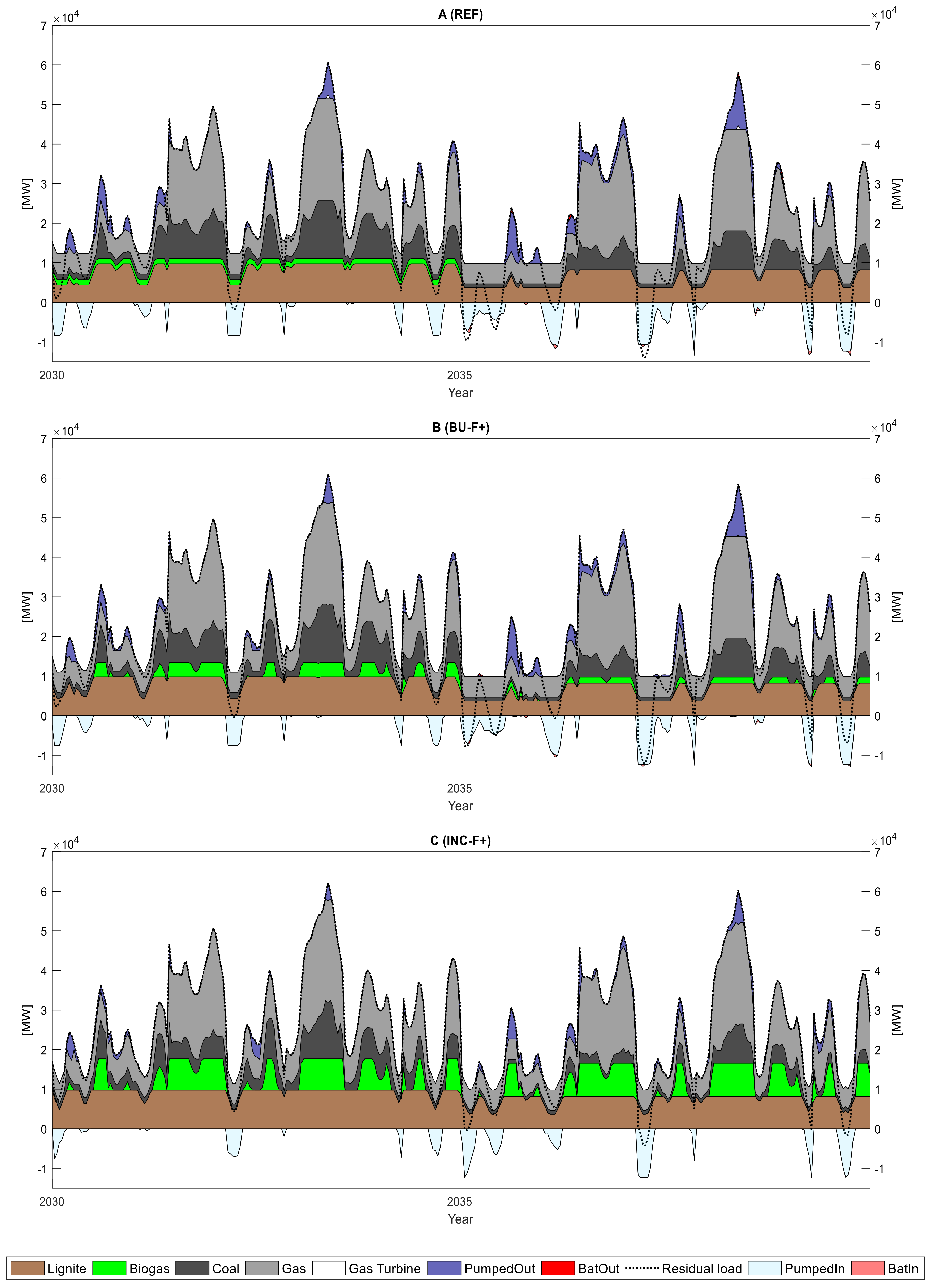
• To analyze the impact of varying proportions of biogas plants on the required power generation from conventional power plants;
• To minimize the residual load demand by the optimization of flexible power generation from biogas plants; and
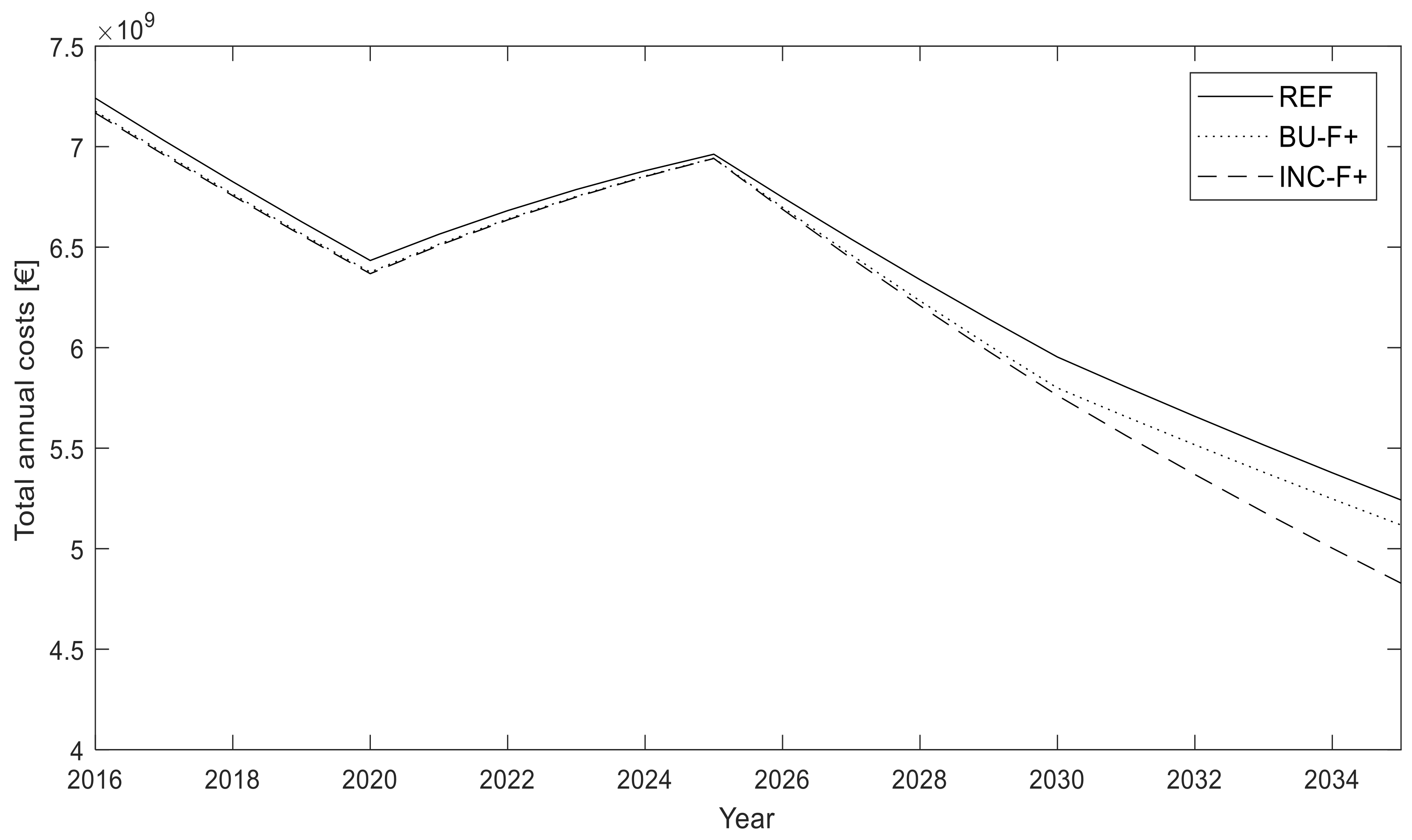
• To examine the effect of flexible power generation from biogas plants on the total costs of the electricity system.

2. Methodology

With regard to the set objectives, we developed a method to describe the residual load curves with three biogas extension paths (Section 2.1), optimized the flexible power generation from biogas plants to reduce the demand for further flexibility options (Section 2.2), and minimized the total costs of the German electricity system for the period of 2016–2035 by using a non-linear optimization model (Section 2.3) taking into account representative days.

The following procedure is based on two significant simplifications. First, Germany’s interconnecting capacities to neighboring countries were neglected. Consequently, demand and supply has to be balanced without the import and export of electricity. Second, the electricity system was described as a “copper plate”, and the curtailment of regional electricity overcapacities and grid losses were not taken into account.

2.1. Selection of Representative Days and Calculation of the Residual Load Curve

In order to select representative days as an input for the optimization model, we used hourly feed-in data from wind and PV plants and the electricity consumption provided by the German transmission system operators [23] and the European Network of Transmission System Operators for Electricity [24] based on the year 2015. Following the methodology of [25], we normalized the hourly feed-in data from intermittent renewable energies and the electricity consumption according to their maximum annual value and used the clustering algorithm to select and weight representative days. In this study, we used four years (2020, 2025, 2030, and 2035) and seven representative days per year to minimize the total costs in the future electricity system. According to [26], a time resolution of 1 h for balancing demand and supply in an electricity system with high proportions of intermittent renewable energies was considered. As a consequence, 672 time slices were used as input data for the optimization of flexible power generation from biogas plants and the minimization of total costs.

2.2. Biogas Extension Paths and Calculation of the Residual Load Curve

Residual load is defined here as the electricity consumption minus the generation by intermittent renewable energies. To calculate the residual load curves for the years considered, we took into account the normalized hourly data of the representative days and increased the installed capacities of intermittent renewable energies. According to [21], we defined three biogas extension paths and calculated the installed capacity and electricity amount of renewable energies:

• Biogas phase out: After their remuneration period of 20 years, biogas plants will start to close down and will phase out in the 2030s.
• Biogas back up: 75 MW of biogas plants will be installed each year. However, due to the closure of existing biogas plants, the installed capacity will decrease to 1500 MW in 2035.
• Biogas increase: The annual deconstruction of existing biogas plants will be taken into account and the installed capacity of biogas plants increased by 100 MW each year for the period of 2016–2035.

To compare the extension paths with each other, the installed capacity and electricity amount of onshore wind plants were adapted to the electricity generated by biogas plants. As a consequence, the proportion of wind onshore plants in extension path biogas phase out has to be higher compared to biogas increase (Figure 1). The net electricity consumption (543.6 TWh∙a⁻¹, Scenario B 2025/2035 [27]) and the generated electricity by biomass (without biogas), hydropower, and other renewables were set to be constant for the period considered (

Table 1. Installed (wind and PV) and rated capacity of renewable energies in each biogas extension path [GW] (own assumptions and references).

Renewable Energy	2016	2020	2025	2030	2035	References
Offshore wind	3.9	6.5	11.0	15.0	19.0	[28,29,30]
PV	41.2	47.3	54.9	57.4	59.9	[27,29,31]
Hydropower	2.2					[29]
Biomass (without biogas)	1.2					[12]
Other renewables	1.3					[29]

). Details of the methodology are given in [21].

2.3. Impact of (Flexible) Biogas Plants on the Residual Load

Flexible power generation from existing biogas plants requires investments in additional CHPU and/or biogas storage technologies, e.g., [8,9]. When biogas production is set to be constant, CHPU capacities above the average biogas production tolerate to shift the power generation over a certain period. To increase the temporal flexibility of biogas plants, the biogas production can also be orientated on the expected power generation [32,33]. The flexible biogas production allows a longer temporal shift of electricity generation during the time of low electricity demand and a longer period of maximum electricity generation during the time of low electricity supply by intermittent renewable energies. For this purpose, according to [34] we took three plant configurations of existing and new biogas plants into consideration (

Table 2. Biogas plant configurations (according to [34]). PQ = power quotient.

Plant Configuration	Flexible Biogas Production	PQ	Biogas Storage Capacity 1	Full Load Hours per Year
Base	Baseload generation
Flex		2	10	4380
Flex+	X

¹ Biogas storage capacity is defined as quotient of storage capacity (m³) and hourly biogas production (m³∙h⁻¹).

): The electricity generated by biogas plants is set to be constant in the plant configuration Base. In plant configuration Flex, the biogas production is set to be constant and the electricity generation is flexible depending on the biogas storage capacity of the biogas plant. Whereas in Flex+, the biogas production and the electricity generation were defined to be flexible to increase the flexibility of biogas plants. When existing biogas plants reach a remaining period of 10 years of remuneration, biogas plants generate flexible power (see EEG 2017, § 50b). Otherwise these are in baseload operation (details see [34]).

To optimize the flexible biogas generation, the model of [34] was used to smooth the residual load curve by using the following objective function:

$$\min f({\left\{p_t\right\}}_t^T|{\left\{r_t\right\}}_t^T)={\displaystyle \sum }_t{\left(r_t-p_t\right)}^2$$

(1)

where p_t is the power generation from biogas plants and r_t is the residual load at each time t over the period T. All details of the model are described in [34].

The optimization was done for each biogas plant configuration and extension path, combining the scenarios considered [34] (

Table 3. Scenarios based on biogas extension paths and plant configurations [34].

Biogas Extension Path	Plant Configuration	Scenario
Increase	Base (B)	INC-B
	Flex (F)	INC-F
	Flex+ (F+)	INC-F+
Back up	Base (B)	BU-B
	Flex (F)	BU-F
	Flex (F+)	BU-F+
Phase out	Base (B)	REF

). The residual load curves for each scenario for the period of 2016–2035 were used as inputs for the non-linear optimization model.

To assess the increasing proportion of biogas plants and their flexible power generation the impact I, defined as the rooted absolute difference between the reference scenario REF and the scenarios considered SCEN, were calculated over the period T [34] (Equation (2)):

$$I\left(f\right)=\sqrt{f\left(REF\right)-f\left(SCEN\right)}$$

(2)

2.4. Minimizing the Total Costs of the Electricity System in Varying Biogas Scenarios

In order to minimize the total costs in the future electricity system a non-linear optimization model is used which simultaneously optimizes the optimal hourly dispatch and the annual investments in conventional power plants and storage technologies. The installed capacity of nuclear, lignite, coal, and gas ([27], Scenario B 2025/2035) is predetermined exogenously for the period of 2016–2035. With regard to the optimal hourly dispatch in each hour and the total costs minimization, the model optimizes, endogenously, additional investments in flexible gas turbines, pumped-storage plants, and battery storage technologies (lithium ion) for balancing demand and supply of the residual load curve including electricity generation from biogas plants. Technical and economic data of storage technologies, such as round-trip efficiency or investments and marginal costs, were also predetermined exogenously.

Most of the operational power system and long-term energy system planning models are represented by linear problems [35], e.g., PLEXOS [36] or TIMES [37]. However, to focus on the time component of costs and benefits within a period of 20 years, we used a non-linear optimization model discounting the interest of all investments and marginal costs. Furthermore, we combined the hourly dispatch of operational power system models by simplifications, as well as the reduction of time slices by representative days and the consideration of 20 years that is part of long-term energy system planning models. The model was implemented in MATLAB (R2016b) using the interior-point algorithm (fmincon). Details of the model are given in the following equations and inequalities.

$$\min {\displaystyle \sum }_t\frac{\left({{\displaystyle \sum }}_{exist}(m{c}_{exist,t}\times {{\displaystyle \sum }}_h{p}_{exist,h,t}\right)+{{\displaystyle \sum }}_{new}(m{c}_{new,t}\times {{\displaystyle \sum }}_h{p}_{new,h,t}+c{c}_{new,t}\times re{q}_{new,t}))}{{\left(1+i_{soc}\right)}^t}$$

(3)

Subject to

$$R{L}_{h,t}-p_{exist,h,t}-p_{new,h,t}\le 0\forall h,t,exist,new$$

(4)

$$re{q}_{stor,t}=cap{0}_{stor}+\max \{cap{0}_{stor};re{q}_{stor,t}\}\forall t,stor$$

(5)

$$re{q}_{GT,t}=\frac{\max \{re{q}_{GT,t=1};re{q}_{GT,t}\}}{a{v}_{GT}}\forall t$$

(6)

$$minP\le p_{conv,h,t}\le maxP\times a{v}_{conv}\forall h,t,conv$$

(7)

$$\left|p_{exist,h,t}-p_{exist,h-1,t}\right|\le \Delta P\forall h,t,exist$$

(8)

$$0\le f{l}_{stor,h,t}\le maxS{C}_{stor}\forall h,t,stor$$

(9)

$$f{l}_{stor,h,t}=fl{0}_{stor}+f{l}_{stor,h-1,t}+p_{storin,h,t}\times \eta -p_{storout,h,t}\forall h,t,stor$$

(10)

$${\displaystyle \sum }_h{p}_{storin,h,t}\times {\eta }_{stor}={\displaystyle \sum }_h{p}_{storout,h,t}\forall t,stor$$

(11)

$$p_{storout,h,t}\le re{q}_{stor,t}\times CF\forall h,t,stor$$

(12)

$${\displaystyle \sum }_h{p}_{exist,h,t}\times FGH{G}_{exist,t}+p_{GT,h,t}\times FGH{G}_{GT,t}+{\displaystyle \sum }_h{p}_{renew,h,t}\times FGH{G}_{renew}\le maxGH{G}_t\forall t,exist,renew$$

(13)

In the objective function (Equation (3)), total costs of existing and new installed conventional power plants, as well as storage technologies, were minimized for the exemplary years and discounted by a social discount rate i_soc. The annual total costs (capital costs cc_t and marginal costs mc_t) between the exemplary years taken into consideration were set to be the same as in the exemplary year before. However, these costs were discounted depending on the year t. Intermittent renewable energies are characterized by marginal costs close to zero. The residual load RL_h,t has to be supplied by the technologies considered in each hour at time h and surplus generation is allowed to occur (Equation (4)). In addition to existing storage technologies cap0_stor, the model allows investments in additional capacities req_stor,t (Equation (5)). The installed capacity of gas turbines was endogenously optimized, regarding to their average availability av_conv (Equation (6)). Furthermore, the power generation by conventional power plants was constrained by the minimum level of power generation minP, the installed capacity maxP, the average availability of conventional power plants av_conv (Equation (7)) and the hourly load change rate ΔP (Equation (8)). In contrast to conventional power plants, the model allows investments in new storage capacities and, therefore, the maximum storage capacity is exclusively restricted to the extension potential of storage technologies maxSC (Equation (9)). In addition, the overall efficiency η of storage technologies was taken into consideration by the charging process p_STORin,h,t (Equation (10)). Due to the consideration of weighting factors and representative days, the annual sum of discharged and charged electricity from storage technologies has to be identical (Equation (11)). The maximum discharging rate is defined as the product of the installed capacity req_STOR,t and the C-factor CF (maximum discharging power relative to its maximum capacity) (Equation (12)). According to the German GHG target values of reduction in the energy system [3], the annual sum of conventional and renewable GHG emissions was restricted by parameter maxGHG_t (Equation (13)). GHG emissions by renewable and conventional power plants including biogas plants were calculated by using GHG emission factors FGHG [38,39]. Annual total costs were linearly interpolated between the selected years; with the exception of the years 2016–2019, those annual costs were set to be identical with the year 2020.

Exogenous economic data and the installed capacity of conventional power plants, as well as the maximum annual GHG emissions are described in

Table 4. Capital and marginal costs of conventional power plants and storage technologies.

Technology	2016	2020	2025	2030	2035	Source
Capital costs (annuity 1) (103 €∙MW−1)						Own calculations according to
Li-ion batteries	149.4	132.6	112.4	96.5	88.8	[40,41,42,43]
Pumped-storage plants	114.0	118.8	125.3	132.2	139.8	[44,45,46]
Gas turbines	38.8	40.5	42.8	45.3	48.0	[47]
Marginal costs (€∙MWh−1)
Nuclear	10.6	10.7	-	-	-	[38,43,48,49,50,51,52,53,54,55]
Lignite	16.1	21.7	28.6	33.6	38.5
Coal	32.9	39.7	48.1	52.9	57.7
Gas	48.5	60.1	74.7	78.7	82.7
Gas turbines	62.2	77.3	95.9	100.6	105.2
Li-ion batteries	2.1	2.2	2.4	2.6	2.8	[44]
Pumped-storage plants	1.5	1.6	1.7	1.8	2.0	[43]

¹ The annuity was calculated by a discount rate of 6.4%. Life time of Li-ion batteries are 15 years (converter) and five years (battery), respectively; of pumped-storage plants are 60 years and of gas turbines are 50 years. Capital costs include the residual value at the end of the year 2035.

and

Table 5. Exogenous installed capacities of conventional power plants and restricted maximum GHG emissions per year. Missing intermediate values were calculated by linear interpolation.

Technology	2016	2020	2025	2030	2035	Source
Installed capacity (MW)
nuclear	10,793	8107	0	0	0	[27,56]
lignite	20,901	17,212	12,600	10,850	9,100
coal	28,661	25,612	21,800	16,400	11,000
gas	28,466					[56], own assumptions
Maximum GHG emissions (109 t·CO2e∙a−1)	331.9	279.6	227.3	175.0	137.1	[3]

. A comprehensive overview of sets, indices, parameters, variables, and assumptions are given in the Appendix A (

Table A1. Sets, indices, parameters and variables considered in the optimization model.

Type	Range	Description	Unit, Instance
Sets and Indices
h ∈ H		Time	Hours (per year)
t ∈ T		Time	Years
exist ∈ EXIST		Existing conventional and pumped-storage plants	Nuclear, lignite, coal, gas and pumped-storage
new ∈ NEW		Additional gas turbines and storage technologies	Gas turbines, pumped-storage and Li-ion batteries
stor ∈ STOR		Storage technologies	Pumped-storage and Li-ion batteries
conv ∈ CONV		Conventional power plants	Nuclear, lignite, coal, gas and gas turbines
Variables
flstor,h,t	[0; SCstor]	Storage filling level	(MWh)
pconv,h,t	[minP; maxP]	Hourly power generation from conventional power plants	(MWh)
pGT,h,t	R ≥ 0	Hourly power generation from gas turbines	(MWh)
pstorin,h,t	R ≥ 0	Hourly charged electricity in storage technologies	(MWh)
pstorout,h,t	R ≥ 0	Hourly discharged electricity by storage technologies	(MWh)
reqGT,t	R ≥ 0	Required installed capacity of gas turbines	(MW)
reqstor,t	[0; maxSCstor]	Required installed capacity of storage technologies	(MW)
Parameters
avconv	[0; 1]	Average conventional power plant availability
cap0stor	R ≥ 0	Initial installed capacity of storage technologies	(MW)
ccconv	R ≥ 0	Capital costs of conventional power plants	(103 €∙MW−1) , Table 4
ccstor	R ≥ 0	Capital costs of storage technologies	(103 €∙MW−1) , Table 4
CFstor	R ≥ 0	C-factor of storage technologies
ΔPconv	[0; 1]	Load change rate of conventional power plants
$\eta$stor	[0; 1]	Roundtrip efficiency of storage technologies
FGHGconv	R ≥ 0	Emission factors of conventional power plants	(kg∙CO2e∙MWh−1)
FGHGrenew	R ≥ 0	Emission factors of renewable energies	(kg∙CO2e∙MWh−1)
fl0stor	R ≥ 0	Initial filling level storage technologies	(MWh)
iea	[0; 1]	Discount rate of economic actors
isoc	[0; 1]	Social discount rate
maxGHG	R ≥ 0	Maximum annual GHG emissions in the electricity system	(109 t∙CO2e∙a−1), Table 5
maxPconv	R ≥ 0	Installed capacity of conventional power plants	(MW)
maxSCstor	R ≥ 0	Maximum potential of storage technologies	(MW)
mcconv	R ≥ 0	Marginal costs of conventional power plants	(€∙MWh−1), Table 4
mcstor	R ≥ 0	Marginal costs of discharging from storage technologies	(€∙MWh−1), Table 4
minPconv	R ≥ 0	Minimum power generation level	(MW)

and

Table A2. Assumptions on conventional power plants, storage technologies, and the rates of discount.

Parameter	Energy Source/Description	Value	Unit	Source/Note
avconv	conventional power plants	0.9		own assumption according to [64]
cap0stor	pumped-storage plants	7600	(MW)	[46]
	Li-ion	0		own assumption
CFstor	pumped-storage plants	0.16		[65]
	Li-ion	1		[66]
ΔPconv	nuclear	21	(% installed capacity h−1)	[67]
	lignite	17
	coal	35
	gas	22
	gas turbine	100		[68]
ηstor	pumped-storage plants	0.8		[43]
	Li-ion	0.95		[40,41]
fl0stor	storage technologies	0.5 × cap0stor× h−1	(MWh)	own assumption
iea	discount rate of economic actors	0.064		According to German energy suppliers, e.g., [69]
isoc	social discount rate	0.03		[70]
maxSCstor	pumped-storage plants	12,310	(MW)	[46]
	Li-ion	15,000		own assumption
minPconv	nuclear	75	(% installed capacity)	[67]
	lignite	45
	coal	10
	gas	20
	gas turbine	0		own assumption, no must-run operation due to increasing role of renewable energies

).

2.5. Sensitivity Analysis

We conducted a sensitivity analysis to show the impact of the different parameters on the total system costs, the investments in flexibility options and the utilization of conventional power plants. To do so, we varied the annuity of lithium-ion batteries, pumped-storage plants, as well as gas turbines, the social discount rate (−40/+40%), and the price of CO₂ per ton (+40/+80%). To calculate the marginal costs of the conventional power plants (Table 4), CO₂ prices of 7.6 €∙t⁻¹ (2015), 21 €∙t⁻¹ (2025), and 31 €∙t⁻¹ (2035) were taken into account [27,48]. Missing values were calculated by linear interpolation.

3. Results

3.1. Seven Representative Days

The algorithm chooses seven representative days given by the electricity consumption and generation by intermittent renewable energies based on the year 2015. As a result, the representative days and the weighting factor of these days are presented in

Table 6. Selected representative days (in ascending order) and weighting factors for the optimization.

Selected Representative Day	Weighting Factor
89	30
105	73
188	80
190	33
311	60
322	36
324	53

. In according to the cluster size of the selected representative days, the weighting factor ensures that extreme days are not overrepresented in the optimization.

3.2. Impact of Biogas Plants on the Residual Load Curve

In all scenarios, the increasing proportion of biogas plants in the future renewable energy portfolio and their flexible power generation smooth the residual load curve for the period considered; consisting of four selected years (

Table 7. The summed impact of biogas plants on the residual load curve for the years 2020, 2025, 2030, as well as 2035 and the defined scenarios (10³ MWh).

Biogas Extension Path	Scenario	Impact
Back up	BU-B	474.8
	BU-F	1080.9
	BU-F+	1184.6
Increase	INC-B	1014.3
	INC-F	1621.9
	INC-F+	1750.1

). Compared to the phase out of biogas plants in the future electricity system, an increasing proportion of biogas plants smooths the residual load curve. Without the flexibility of biogas plants, the substitution of onshore wind plants by baseload biogas plants also smooths the residual load curve in both extension paths characterized by an increasing proportion of biogas plants. Nevertheless, the residual load curve becomes smoother when the electricity generation by biogas plants is flexibilized. In the biogas extension paths back up and increase, the combination of flexible electricity generation and gas production achieves the best results. The smoothing effect is impacted to the largest extent in the scenario INC-F+ when the proportion of biogas plants are increasing and the gas production is flexibilized. This is why the flexible gas production is allowed to shift the electricity generation and to stop them over a longer period of positive and negative residual load, respectively.

In the extension path back up, the impact varies between 474.8 and 1184.6 × 10³ MWh over the years 2020, 2025, 2030, and 2035. In scenario BU-F, the flexible electricity generation from biogas plants impact is calculated to be 1080.9 × 10³ MWh, which are more than two times higher than in the baseload electricity generation (BU-B). When the gas production is also flexibilized, the smoothing effect is increasing to 1184.6 × 10³ MWh (BU-F+). The results of extension path increase are of similar characteristic as the ones given in biogas extension path back up. The higher the flexibility from biogas plants the higher the impact on the residual load curve. Due to a higher proportion of dispatchable biogas plants compared to intermittent onshore wind plants, the impact is increased up to 1750.1 × 10³ MWh. To conclude, flexible power generation from biogas plants increase this effect, though, the marginal benefit of additional biogas plants in the electricity system is decreasing when their proportion becomes higher.

3.3. Impact of Biogas Plants on the Future German Electricity System

3.3.1. Impact of Biogas Plants on the Total Costs in the Electricity System

Depending on the impact of varying extension paths and modes of operations of biogas plants on the residual load curve, different total costs were optimized in the scenarios (

Table 8. The total costs in the electricity system for the period 2016–2035 and scenarios defined (10⁹ €).

Biogas Extension Path	Scenario	Total Costs
Phase out	REF	127.353
Back up	BU-B	127.099
	BU-F	125.929
	BU-F+	125.677
Increase	INC-B	126.273
	INC-F	124.654
	INC-F+	124.524

). The highest total costs occur in the extension path phase out. The summed and discounted annual costs are about 127.35 × 10⁹ € for the period considered. An increasing proportion of biogas plants in the future German electricity system decreases the total costs, without taking the costs of biogas plants into account. In the extension path back up, the total costs vary between 127.10 and 125.68 × 10⁹ € and are comparably lower than the reference scenario. Furthermore, the results indicate that biogas plants should operate as flexibly as possible to decrease the total costs. The lowest results within the extension paths were achieved in the Flex+ mode of operation (BU-F+ and INC-F+). Overall, the lowest total system costs were calculated in the extension path with the highest rate of construction of new biogas plants (increase). In the scenario INC-F+, the total costs were the lowest characterized by 124.52 × 10⁹ €. The highest total costs were calculated in the baseload mode of operation (INC-B).

As analyzed in Section 3.2, the marginal utility in the extension path with the lower construction of new biogas plants (extension path back up) is higher than in the extension path increase. This results from the fact that the majority of existing biogas plants starts to close down between 2025 and 2030 (see Figure 1). Consequently, the differences of the installed capacities of biogas plants and the discounted annual costs in the scenarios start to become significant from the year 2030 onwards (Figure 2). As a result, if the costs of biogas plants are taken into consideration, the costs of additional biogas plants in the extension path increase might be higher than their additional benefit, taking the period of 2016–2035 into account.

The differences of discounted total annual costs can be explained by two reasons: the impact of biogas plants on (i) the demand for additional flexibility options and on (ii) the utilization of conventional power plants.

3.3.2. Impact of Biogas Plants on the Demand for Additional Flexibility Options

In general, the increasing proportion of biogas plants, especially their flexible power generation, decreases the demand for additional flexibility options (

Table 9. Accumulated additional installed capacities of flexibility options in the electricity system for the years and scenarios defined (MW).

Scenario	Pumped-Storage				Li-ion				Gas Turbine
Year	2020	2025	2030	2035	2020	2025	2030	2035	2020	2025	2030	2035
REF	0	0	745	4710	0	0	3	1218	0	0	949	949
BU-B	0	0	660	4710	0	1	3	1040	0	0	758	758
BU-F	0	0	0	4710	0	0	0	770	0	0	0	278
BU-F+	0	0	0	4710	0	0	0	660	0	0	0	389
INC-B	0	0	0	4710	2	2	4	83	0	1	20	20
INC-F	0	0	0	4710	0	1	1	3	0	0	1	1
INC-F+	0	0	0	4709	0	1	1	2	0	1	1	1

). Under the assumptions considered, in all scenarios (with the exception of REF, BU-B, and INC-B) the installed capacities of conventional power plants and existing storage technologies will be sufficient until the end of the 2020s. In the reference scenario, the phase out of biogas plants leads to the investment of additional pumped-storage plants and gas turbines in the year 2030. Similar results are achieved in the scenarios BU-B and INC-B. In all other scenarios, additional flexibility options are required (significant) starting from the year 2035 onwards. According to the achieved results, an increasing proportion of biogas plants substitutes the demand of Li-ion batteries and gas turbines in the future electricity systems. Pumped-storage plants are the cheapest solution to provide flexibility, therefore, the investments in pumped-storage plants were maximized by the optimization model. In our calculations, we allowed a maximum additional capacity of 4710 MW of pumped-storage plants; due to geographic circumstances, their potential is limited. Consequently, in all scenarios, the potential of pumped-storage plants was utilized and more cost-intensive flexibility options were substituted by biogas plants. As a result, there is no impact of varying biogas extension paths on the demand for additional flexibility options in the 2020s.

3.3.3. Impact of Biogas Plants on the Utilization of Conventional Power Plants and GHG Emissions

In addition, an increasing proportion of (flexible) biogas plants reduces the demand of conventional power plants, which are characterized by comparable high marginal costs. In

Table A4. Utilization of the conventional power plants and the storage technologies in the scenarios and years considered. Furthermore, the annual surplus generation is shown. Values of storage technologies describe the discharged amount of electricity (TWh∙a⁻¹). Values are rounded.

Year	Scenario	Nuclear	Lignite	Coal	Gas	Pumped-Storage	Li-ion	Gas turbine	Surplus
2020	REF	63.57	130.43	75.05	45.38	9.77	0	0	0.01
	BU-B	63.49	130.97	74.65	45.34	9.94	0	0	0.09
	BU-F	63.57	131.80	73.36	45.04	7.67	0	0	0
	BU-F+	63.83	132.24	72.76	44.97	7.65	0	0	0
	INC-B	63.56	131.03	74.55	45.32	10.00	0	0	0.08
	INC-F	63.82	132.31	72.74	44.94	7.69	0	0	0
	INC-F+	63.82	132.90	72.19	44.94	7.87	0	0	0
2025	REF	0	95.85	96.50	84.36	2.65	0	0	0
	BU-B	0	96.01	95.54	85.13	2.47	0	0	0
	BU-F	0	97.56	93.52	85.61	2.53	0	0	0
	BU-F+	0	97.88	93.26	85.38	1.81	0	0	0
	INC-B	0	96.56	93.78	86.32	2.40	0	0	0
	INC-F	0	98.34	91.74	86.25	1.09	0	0	0
	INC-F+	0	97.56	92.88	85.74	0.49	0	0	0
2030	REF	0	75.77	54.17	105.20	7.72	0	0.05	1.37
	BU-B	0	76.28	52.58	105.99	7.40	0	0.04	1.15
	BU-F	0	77.35	51.95	104.73	6.09	0	0	0.61
	BU-F+	0	77.87	51.33	104.78	5.89	0	0	0.61
	INC-B	0	77.89	46.93	109.06	6.37	0	0.01	0.40
	INC-F	0	81.77	42.92	108.09	3.54	0	0	0
	INC-F+	0	82.05	42.55	108.19	3.61	0	0	0
2035	REF	0	57.88	32.49	108.66	14.26	0.46	0.05	7.75
	BU-B	0	58.26	31.45	108.12	14.08	0.40	0.04	6.58
	BU-F	0	57.91	32.54	106.60	13.63	0.47	0.02	5.89
	BU-F+	0	58.23	32.49	105.92	13.57	0.34	0.02	5.50
	INC-B	0	60.09	25.49	107.90	12.96	0.04	0	2.51
	INC-F	0	62.72	24.99	102.43	9.20	0	0	0.11
	INC-F+	0	65.88	21.05	103.24	9.29	0	0	0.11

(see Appendix A) the utilization of conventional power plants and storage technologies is shown. Compared to the reference scenario, biogas plants reduce the utilization of coal-fired and gas-fired power plants and increase the supply of baseload generation power plants (nuclear or/and lignite). This effect is also shown in Figure 3. The increasing proportion and flexible power generation from biogas plants smooths the residual load curve and baseload generation power plants are better utilized. However, lignite-fired power plants have the highest GHG emissions and increasing full load hours lead to additional GHG emissions. In this study, we took annual maximum GHG emissions into account. Therefore, the utilization of lignite-fired power plants with low marginal costs is limited and the GHG emissions are similar or identical, respectively, in all scenarios (

Table A5. GHG emissions of the conventional power plants in the scenarios and years considered (10⁹ t·CO₂e∙a⁻¹). Values are rounded.

Year	Scenario	Nuclear	Lignite	Coal	Gas	Gas Turbine	Renewables	Sum
2020	REF	0	136.87	66.94	18.33	0	7.66	229.80
	BU-B	0	137.44	66.59	18.32	0	7.85	230.19
	BU-F	0	138.31	65.44	18.20	0	7.85	229.80
	BU-F+	0	138.76	64.90	18.17	0	7.85	229.68
	INC-B	0	137.49	66.50	18.31	0	7.92	230.22
	INC-F	0	138.83	64.89	18.15	0	7.92	229.79
	INC-F+	0	139.46	64.39	18.15	0	7.92	229.93
2025	REF	0	99.31	86.08	34.08	0	7.82	227.30
	BU-B	0	99.48	85.22	34.39	0	8.21	227.30
	BU-F	0	101.08	83.42	34.59	0	8.21	227.30
	BU-F+	0	101.41	83.19	34.49	0	8.21	227.30
	INC-B	0	100.04	83.65	34.87	0	8.73	227.30
	INC-F	0	101.89	81.83	34.84	0	8.73	227.30
	INC-F+	0	101.08	82.85	34.64	0	8.73	227.30
2030	REF	0	77.50	48.32	42.50	0.03	6.65	175.00
	BU-B	0	78.03	46.90	42.82	0.02	7.23	175.00
	BU-F	0	79.12	46.34	42.31	0	7.23	175.00
	BU-F+	0	79.65	45.79	42.33	0	7.23	175.00
	INC-B	0	79.67	41.86	44.06	0	9.41	175.00
	INC-F	0	83.64	38.28	43.67	0	9.41	175.00
	INC-F+	0	83.93	37.96	43.71	0	9.41	175.00
2035	REF	0	58.44	28.98	43.89	0.03	5.74	137.08
	BU-B	0	58.81	28.05	43.68	0.02	6.51	137.08
	BU-F	0	58.47	29.02	43.07	0.01	6.51	137.08
	BU-F+	0	58.79	28.98	42.79	0.01	6.51	137.08
	INC-B	0	60.67	22.73	43.59	0	10.08	137.08
	INC-F	0	63.32	22.29	41.38	0	10.08	137.08
	INC-F+	0	66.51	18.77	41.71	0	10.08	137.08

).

4. Discussion

4.1. Applied Methodologies

The assessment of future extension paths of renewable energies is often carried out by the consideration of selected years instead of a period. However, political decision-makers have to evaluate their investments in renewable energies according to the period that reflects the impact of economic decisions. Therefore, we considered a period of 20 years, which is consistent with the remuneration period of the EEG for renewable energies in Germany. Taking the period into account also allows identifying an advantageous time of the investment and prevents early investments in technologies, e.g., characterized by a high cost-reduction. In addition, dispatchable biogas plants are associated with a higher LCOE compared to intermittent renewable energies or flexibility options, such as battery storage. Nevertheless, the LCOE does not typically consider the total system costs of system integration of intermittent renewable energies by using flexible conventional power plants or other technological solutions. Comparing storage technologies with biogas plants, the costs and time of energy supply by conventional or renewable energies also have to be taken into account. Consequently, the total system costs are a more appropriate approach to assess the proportion of biogas plants in the future renewable energy portfolio and their dispatchable power generation.

In addition, compared to the results of [22] we also showed that flexible power generation from biogas plants reduces the total costs in the German electricity system. However, they compared the total system costs between baseload and endogenously-optimized flexible power generation from biomass plants while the electricity was set to be constant, whereas in this paper, the proportion of biogas plants in the future electricity system was varied. In addition, we defined the design of the flexible biogas plants exogenously. Nevertheless, regarding the total system costs, the economic feasibility of flexible power generation from biogas plants compared to their baseload operation cannot yet be finally assessed. To do so, the marginal and capital costs of the renewable energies in all extension paths have to be used for a cost-benefit analysis in the period considered.

4.2. Discussion of Limitations

Germany was simplified as a “copper plate”, losing energy by grid bottlenecks or the curtailment of renewable energies were neglected. However, the curtailment of wind energy has been increasing since 2009 [57] and the German government decided to limit the extension of wind power plants concentrated in the north of Germany (EEG 2017, § 36c). In addition, the requirement for flexibility options in the future electricity was overestimated. The import and export of electricity to neighboring countries smooths the residual load curve and was not taken into account. In general, the demand for dispatchable power plants can be considered as conservative.

In this paper, the current framework for the energy sector was taken as a basis. This regards the future expansion of renewable energies and the energy demand in the above mentioned period. Though, the framework conditions can be subject to a rapid change, as shown in the past amendments of the EEG, e.g., the shift from feed-in tariffs determined by the German government towards a tendering system. In the same way, according to the set goals of the German Climate Action Plan and the future electrification of the mobility and heating sector, the extension paths of renewable energies has to be increased by the German government in a timely manner for a decarbonization of the energy system until the year 2050. As a result, the demand for flexibility options is growing more rapidly than considered in this study. In addition, due to the increasing electrification of the heating and mobility sector (sector coupling), as well as advanced intermittent renewable energies, e.g., weak wind turbines, the future electricity demand and supply curve may be subject to change. Despite increasingly efficient electricity use, the overall demand may be higher than forecasted by the German transmission system operators. According to the renewable energy extension target values, an increasing electricity demand leads to a higher extension of (intermittent) renewable energies that have to be balanced by additional flexibility options.

Biogas plants are generating flexible electricity to decrease the demand for conventional power plants and storage technologies. Nonetheless, cost-intensive flexibility of small biogas plants using mainly manure and additional technical efforts could limit the flexible power generation in order to integrate intermittent renewable energies. However, small biogas plants using manure are characterized by additional benefits, such as low GHG emissions [58] and lower external costs. In summary, biogas plant operators will maximize their return on investment and the benefit from dispatchable renewable energies will be lower than that considered in this study. Last, electricity generation from biogas plants was compared with marginal costs and investments in conventional power plants, Li-ion batteries, and pumped-storage plants by using representative days. Power-to-gas can be also one option for the seasonal storage of intermittent renewable energies; though, the use of representative days does not allow the consideration of seasonal storage technologies. However, due to the low surplus generation in the period considered, power-to-gas becomes more important in electricity systems characterized by a higher proportion of intermittent renewable energies.

4.3. Optimal System Contribution of Biogas

In our calculations, the biogas extension path back up achieved a higher marginal utility than the biogas extension path increase. Furthermore, in the extension path back up, the installed capacity of biogas plants is 1.500 MW and they contribute to 1.2% of Germany’s net electricity consumption in the year 2035 (6.6 TWh). The annual baseload operation of other biomass plants is about 10.6 TWh. In addition, the installed capacity of biogas plants in the extension path back up is based on the study of Repenning et al. [59], who calculated the installed capacity of biogas plants in 2035 to achieve the ambitious GHG reduction target in Germany of 95% by 2050 compared to the reference year 1990. In other publications, a higher amount of electricity generated by biogas plants is taken into account. For example, Eltrop et al. [22] considered an annual electricity generation from biogas plants of 46 TWh in all scenarios characterized by a proportion of 40%, 60%, and 80% of renewable energies, whereas Holzhammer [20] based his calculations of flexible electricity generation from biogas plants on an annual electricity amount between 30.5 and 52 TWh in 2030. Schill [60] took flexible electricity generation from biomass plants of 59 TWh∙a⁻¹ into consideration and calculated the storage demand in Germany in 2032 and 2050. Greenpeace [61] analyzed Germany’s electricity and heating sectors based on 100% renewable energies in the year 2050; they took an annual (flexible) electricity generation from biomass plants of 45 TWh into account. To summarize, an increasing system contribution of biogas plants, which was examined in the biogas extension path increase, achieved a comparable lower decrease of the total annual costs in Germany’s electricity system. Compared to the above-mentioned studies, the (flexible) electricity generation from biogas and biomass plants, respectively, considered in these studies is similar to the biogas extension path increase; characterized by an electricity generation from biogas plants of 36.8 TWh and 10.6 TWh from other biomass plants in baseload generation.

4.4. Sensitivity Analysis

In

Table 10. Results of the sensitivity analysis: additional installed capacities of flexibility options in the scenario BU-F+ and the year 2035.

Parameter		Pumped-Storage	Li-ion	Gas Turbine
Capital costs of	Li-ion (−40%)	4710	660	389
	Li-ion (+40%)	4710	0	1048
	Pumped-storage (−40%)	4710	116	933
	Pumped-storage (+40%)	4710	660	389
	Gas turbine (−40%)	4710	286	762
	Gas turbine (+40%)	4710	660	389
Social discount rate (−40%)		4710	660	389
Social discount rate (+40%)		4710	660	389
Price of CO2 (+40%)		4710	660	389
Price of CO2 (+80%)		4710	660	389

, we show the additional installed capacities of flexibility options depending on the parameter varied in the sensitivity analysis. In all cases, the investments in pumped-storage plants were unchanged, whereas, in three cases, different installed capacities of Li-ion batteries and gas turbines were needed to supply the electricity demand in the scenario BU-F+ and the year 2035. With the exception of increased Li-ion and decreased gas turbine capital costs, no additional investments in Li-ion batteries and/or gas turbines were made. The sum of both flexibility options was 1048 MW for all varied parameters. Furthermore, in all cases, varied parameters did not lead to significant changes of the utilization of conventional power plants. Although, the CO₂ price was increased by 80%, conventional power plants characterized by lower GHG emissions were not utilized more often.

With regard to the total system costs, the variation of the annuity of flexibility options had a low effect on the results (Figure 4). The highest impact was achieved by the variation of the annuity of pumped-storage plants, whereas different social discount rates and the CO₂ prices (Figure 5) are characterized by a higher sensitivity and lead to significantly higher and lower total system costs, respectively.

5. Conclusions and Policy Implications

In this study, we analyzed the impacts of varying biogas plants extension paths, including Germany’s existing biogas plants, and modes of operation on the total system costs in the period of 2016–2035 by using a non-linear optimization model. We found that an increasing proportion of (flexible) biogas plants in the future German electricity system reduces the demand of storage technologies and flexible conventional power plants to supply the demand. Without taking into account the capital and marginal costs of biogas plants, they can be a cost-effective flexibility option (compared to other technologies).

Firstly, the replacement of intermittent onshore wind capacities by dispatchable biogas plants smooths the residual load curve and reduces the demand for further flexibility options. Secondly, the operation of biogas plants should be as flexible as possible to increase the effect on the future residual load curve and the reduction of the total system costs. However, the findings underline that the biogas extension path back up may be a more economically feasible way to integrate intermittent renewable energies into the electricity system than the continuous increase in the extension path increase. Regarding the total costs, the marginal utility in the extension path increase was lower than in the extension path back up and emphasizes, under the assumptions considered, a constant increase of biogas plants may lead to additional system costs. Our model results specify that Germany’s electricity system is characterized by sufficient capacities of flexibility and additional flexibility options are needed from about the year 2030 onwards. Thus, in the short-term, there is no need to implement further flexibility options when the extension paths of renewable energies and the decrease of the installed capacity of conventional power plants remain unchanged. However, due to Germany’s ambitious GHG reduction target values and the goals of the Paris Agreement, the utilization and the installed capacity of lignite-fired, as well as coal-fired power plants have to be reduced more rapidly [62]. Furthermore, the decarbonization of the energy systems also requires the use of renewable electricity in the heating and mobility sectors [63], whereby extension of intermittent renewable energies should be further enhanced, compared to the defined annual increase of renewable energies in the EEG (EEG 2017, § 4). Depending on the capacities of conventional and renewable capacities, additional flexibility options may be needed before 2030. To summarize, based on the future extension paths of renewable energies and the installed capacity of conventional power plants, (flexible) biogas plants can be a cost-effective subset of future flexibility options to integrate intermittent renewable energies into the electricity system.

From the broader perspective of policymakers, we recommend the following strategies:

• The economic assessment of flexibility options in the electricity system has to include the interactions between these options and all conventional, as well as renewable energy provision technologies, within Germany’s electricity system. From the year 2030 onwards, flexible power generation from biogas plants can be an option to decrease the total system costs in Germany’s electricity system.
• The optimal installed capacity and mode of operation of biogas plants depends on the development of conventional and (intermittent) renewable energies in the future electricity system.
• To increase the market penetration of flexible power generation from biogas plants, additional market revenues are needed. This can be achieved by the reduction of conventional power plants in baseload operation.
• Due to the limited potential of biomass, the economic assessment of biomass use in the energy system should also be taken into account in different areas of application: e.g., the production of basic chemicals based on biomass might be necessary if GHG emissions are reduced up to 95% by 2050.

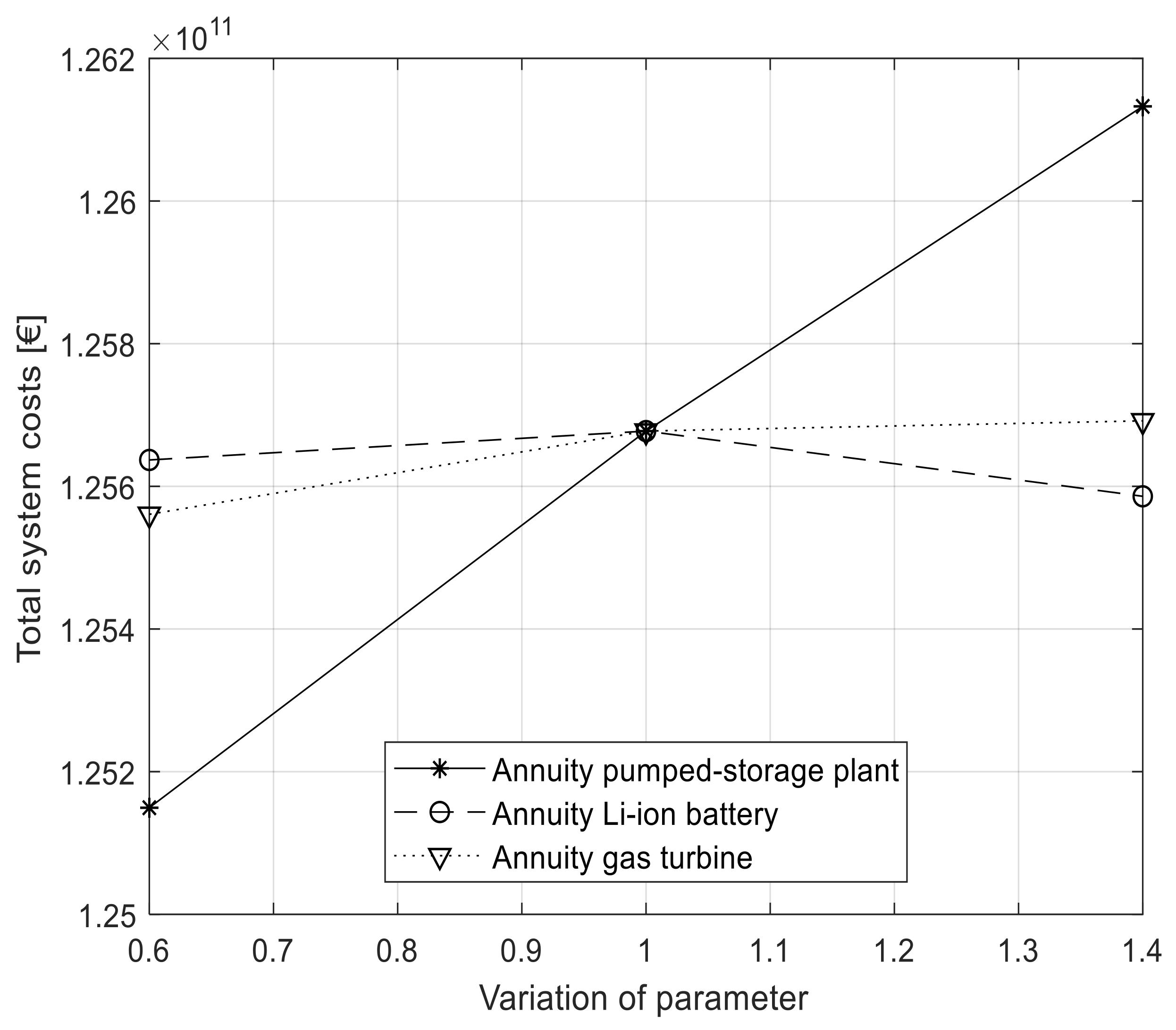
For further research, we suggest a cost-benefit analysis to finally assess the most cost-effective extension path and mode of generation of biogas plants in the future German electricity system. Therefore, the varying costs of the intermittent renewable energies and of biogas plants, respectively, in all scenarios have to be taken into account. A cost-benefit analysis would enable a comprehensive economic assessment that considers the discounted costs and benefits over the period considered.

References

1. United Nations (UN). Adoption of the Paris Agreement FCCC/CP/2015/L.9/Rev.1 (UNFCCC, 2015); United Nations: New York, NY, USA, 2015. [Google Scholar]
2. Rogelj, J.; Luderer, G.; Pietzcker, R.C.; Kriegler, E.; Schaeffer, M.; Krey, V.; Riahi, K. Energy system transformations for limiting end-of-century warming to below 1.5 °C. Nat. Clim. Chang. 2015, 5, 519–527. [Google Scholar] [CrossRef]
3. The Federal Ministry of the Environment, Nature Conservation, Building and Nuclear Safety (BMUB). Climate Action Plan 2050—Principles and Goals of the German Government’s Climate Policy; Federal Ministry for the Environment, Nature Conservation, Building and Nuclear Safety: Bonn, Germany, 2016.
4. Renewable Energy Sources Act (EEG) 2017; German Parliament: Bonn, Germany, 2016.
5. International Energy Agency (IEA). Harnessing Variable Renewables: A Guide to the Balancing Challenge; OECD Publishing and International Energy Agency: Paris, France, 2011. [Google Scholar]
6. Lund, P.D.; Lindgren, J.; Mikkola, J.; Salpakari, J. Review of energy system flexibility measures to enable high levels of variable renewable electricity. Renew. Sustain. Energy Rev. 2015, 45, 785–807. [Google Scholar] [CrossRef]
7. BMWi. Development of Renewable Energy in Germany 2016—Graphs and Diagramms Based on Working Group on Renewable Energy-Statistics (AGEE-Stat); as at February 2017. Federal Ministry for Economic Affairs and Energy, 2017. Available online: http://www.erneuerbare-energien.de/EE/Redaktion/DE/Bilderstrecken/entwicklung-der-erneuerbaren-energien-in-deutschland-im-jahr-englisch.html (accessed on 9 June 2017).
8. Szarka, N.; Scholwin, F.; Trommler, M.; Fabian Jacobi, H.; Eichhorn, M.; Ortwein, A.; Thrän, D. A novel role for bioenergy: A flexible, demand-oriented power supply. Energy 2013, 61, 18–26. [Google Scholar] [CrossRef]
9. Lauer, M.; Dotzauer, M.; Hennig, C.; Lehmann, M.; Nebel, E.; Postel, J.; Szarka, N.; Thrän, D. Flexible power generation scenarios for biogas plants operated in Germany: Impacts on economic viability and GHG emissions. Int. J. Energy Res. 2017, 41, 63–80. [Google Scholar] [CrossRef]
10. Thrän, D.; Dotzauer, M.; Lenz, V.; Liebetrau, J.; Ortwein, A. Flexible bioenergy supply for balancing fluctuating renewables in the heat and power sector—A review of technologies and concepts. Energy Sustain. Soc. 2015, 5, 35. [Google Scholar] [CrossRef]
11. Horschig, T.; Adams, P.W.R.; Röder, M.; Thornley, P.; Thrän, D. Reasonable potential for GHG savings by anaerobic biomethane in Germany and UK derived from economic and ecological analyses. Appl. Energy 2016, 184, 840–852. [Google Scholar] [CrossRef]
12. Scheftelowitz, M.; Rensberg, N.; Denysenko, V.; Daniel-Gromke, J.; Stinner, W.; Hillebrand, K.; Naumann, K.; Peetz, D.; Hennig, C.; Thrän, D.; et al. Stromerzeugung aus Biomasse (Vorhaben IIa Biomasse)—Zwischenbericht Mai 2015; DBFZ/UFZ/IWES: Leipzig, Germany, 2015. [Google Scholar]
13. Urzúa, I.A.; Olmedo, J.C.; Sauma, E.E. Impact of intermittent non-conventional renewable generation in the costs of the Chilean main power system. Renew. Sustain. Energy Rev. 2016, 60, 810–821. [Google Scholar] [CrossRef]
14. Jacobson, M.Z.; Delucchi, M.A.; Cameron, M.A.; Frew, B.A. Low-cost solution to the grid reliability problem with 100% penetration of intermittent wind, water, and solar for all purposes. Proc. Natl. Acad. Sci. USA 2015, 112, 15060–15065. [Google Scholar] [CrossRef] [PubMed]
15. Budischak, C.; Sewell, D.; Thomson, H.; Mach, L.; Veron, D.E.; Kempton, W. Cost-minimized combinations of wind power, solar power and electrochemical storage, powering the grid up to 99.9% of the time. J. Power Sources 2013, 225, 60–74. [Google Scholar] [CrossRef] [Green Version]
16. Heide, D.; Greiner, M.; Bremen, L.; von Hoffmann, C. Reduced storage and balancing needs in a fully renewable European power system with excess wind and solar power generation. Renew. Energy 2011, 36, 2515–2523. [Google Scholar] [CrossRef]
17. Pfenninger, S.; Keirstead, J. Renewables, nuclear, or fossil fuels? Scenarios for Great Britain’s power system considering costs, emissions and energy security. Appl. Energy 2015, 152, 83–93. [Google Scholar]
18. Brouwer, A.S.; van den Broek, M.; Zappa, W.; Turkenburg, W.C.; Faaij, A. Least-cost options for integrating intermittent renewables in low-carbon power systems. Appl. Energy 2016, 161, 48–74. [Google Scholar] [CrossRef]
19. Zakeri, B.; Rinne, S.; Syri, S. Wind Integration into Energy Systems with a High Share of Nuclear Power? What Are the Compromises? Energies 2015, 8, 2493–2527. [Google Scholar] [CrossRef]
20. Holzhammer, U. Biogas in einer Zukünftigen Energieversorgungsstruktur mit hohen Anteilen Fluktuierender Erneuerbarer Energien. Ph.D Thesis, Universität Rostock, Rostock, Germany, 2015. [Google Scholar]
21. Lauer, M.; Thrän, D. Biogas plants and surplus generation: Cost driver or reducer in the future German electricity system? Energy Policy 2017, 109, 324–336. [Google Scholar] [CrossRef]
22. Eltrop, L.; Fleischer, B.; Härdtlein, M.; Panic, O.; Maurer, C.; Daiber, R.; Dieter, H.; Beirow, M.; Spörl, R. Speicherung und Flexible Betriebsmodi zur Schonung Wertvoller Ressourcen und zum Ausgleich von Stromschwankungen bei hohen Anteilen Erneuerbarer Energien in Baden-Württemberg (BioenergieFlex BW); Landesanstalt für Umwelt Baden-Württemberg: Karlsruhe, Germany, 2016. [Google Scholar]
23. Übertragungsnetzbetreiber (ÜNB). Veröffentlichungen zur Marktprämie nach § 73 Abs. 3 EEG in Verbindung mit Anlage 1 Nr. 3 EEG. Informationsplattform der Deutschen Übertragungsnetzbetreiber, 2017. Available online: https://www.netztransparenz.de/EEG/Marktpraemie (accessed on 26 June 2017).
24. ENTSO-E. Hourly Load Values for a Specific Country for a Specific Month (in MW). European Network of Transmission System Operators for Electricity, 2017. Available online: https://www.entsoe.eu/db-query/consumption/mhlv-a-specific-country-for-a-specific-month (accessed on 26 June 2017).
25. Nahmmacher, P.; Schmid, E.; Hirth, L.; Knopf, B. Carpe diem: A novel approach to select representative days for long-term power system modeling. Energy 2016, 112, 430–442. [Google Scholar] [CrossRef]
26. Pina, A.; Silva, C.; Ferrão, P. Modeling hourly electricity dynamics for policy making in long-term scenarios. Energy Policy 2011, 39, 4692–4702. [Google Scholar] [CrossRef]
27. NEP. Netzentwicklungsplan Strom 2025, Version 2015; Zweiter Entwurf der Übertragungsnetzbetreiber; 50 Hertz Transmission GmbH, Amprion GmbH, TenneT TSO GmbH, TransnetBW GmbH: Berlin, Germany, 2016. [Google Scholar]
28. Lüers, S.; Rehfeldt, K. Status des Offshore-Windenergieausbaus in Deutschland, Gesamtjahr 2015; Deutsche WindGuard: Varel, Germany, 2016. [Google Scholar]
29. AG Energiebilanzen. Stromerzeugung nach Energieträgern 1990–2015 (Stand 28.01.2016); AG Energiebilanzen: Berlin, Germany, 2016. [Google Scholar]
30. BMWi. EEG-Novelle 2016—Eckpunktepapier. 8. Dezember 2015; Federal Ministry for Economic Affairs and Energy: Berlin, Germany, 2015.
31. BNetzA. Datenmeldungen und EEG-Vergütungssätze für Photovoltaikanlagen—Aktuelle Veröffentlichung der PV-Meldezahlen, Bundesnetzagentur for Electricity, Gas, Telecommunications, Post and Railway. 2016. Available online: http://www.bundesnetzagentur.de/DE/Sachgebiete/ElektrizitaetundGas/Unternehmen_Institutionen/ErneuerbareEnergien/Photovoltaik/DatenMeldgn_EEG-VergSaetze/DatenMeldgn_EEG-VergSaetze_node.html (accessed on 22 June 2016).
32. Mauky, E.; Weinrich, S.; Jacobi, H.-F.; Nägele, H.-J.; Liebetrau, J.; Nelles, M. Demand-driven biogas production by flexible feeding in full-scale—Process stability and flexibility potentials. Anaerobe 2017, 46, 86–95. [Google Scholar] [CrossRef] [PubMed]
33. Grim, J.; Nilsson, D.; Hansson, P.-A.; Nordberg, Å. Demand-Orientated Power Production from Biogas: Modeling and Simulations under Swedish Conditions. Energy Fuels 2015, 29, 4066–4075. [Google Scholar] [CrossRef]
34. Lauer, M.; Röppischer, P.; Thrän, D. Flexible Biogas Plants as Servant for Power Provision Systems with High Shares of Renewables: Contributions to the Reduction of the Residual Load in Germany; ETA-Florence Renewable Energies: Firenze, Italy, 2017. [Google Scholar]
35. Collins, S.; Deane, J.P.; Poncelet, K.; Panos, E.; Pietzcker, R.C.; Delarue, E.; Gallachóir, B.P.Ó. Integrating short term variations of the power system into integrated energy system models: A methodological review. Renew. Sustain. Energy Rev. 2017, 76, 839–856. [Google Scholar] [CrossRef]
36. Energy Exemplar. PLEXOS® Integrated Energy Model. 2017. Available online: https://energyexemplar.com/ (accessed on 21 June 2017).
37. Loulou, R.; Lehtilä, A.; Kanudia, A.; Remme, U.; Goldstein, G. Documentation for the TIMES Model—Part II; International Energy Agency: Paris, France, 2016. [Google Scholar]
38. Icha, P.; Kuhs, G. Entwicklung der Spezifischen Kohlendioxid-Emissionen des Deutschen Strommix in den Jahren 1990 bis 2014—Climate Change 09/2015; Umweltbundesamt: Dessau-Roßlau, Germany, 2015. [Google Scholar]
39. Memmler, M.; Schrempf, L.; Hermann, S.; Schneider, S.; Pabst, J.; Dreher, M. Emissionsbilanz Erneuerbarer Energieträger—Bestimmung der Vermiedenen Emissionen im Jahr 2013, Climate Change 29/2014; Umweltbundesamt: Dessau-Roßlau, Germany, 2014. [Google Scholar]
40. Hewicker, C.; Raadschelders, J.; Werner, O.; Ebert, M.; Engelhardt, C.; Mennel, T.; Verhaegh, N. Energiespeicher in der Schweiz: Bedarf, Wirtschaftlichkeit und Rahmenbedingungen im Kontext der Energiestrategie 2050; Bundesamt für Energie: Bern, Switzerland, 2013. [Google Scholar]
41. Ausfelder, F.; Beilmann, C.; Bertau, M.; Bräuninger, S.; Heinzel, A.; Hoer, R.; Koch, W.; Mahlendorf, F.; Metzelthin, A.; Peuckert, M.; et al. Energiespeicherung als Element einer sicheren Energieversorgung. Chem. Ing. Tech. 2015, 87, 17–89. [Google Scholar] [CrossRef]
42. Fuchs, G.; Lunz, B.; Leuthold, M.; Sauer, D.U. Technology Overview on Electricity Storage—Overview on the Potential and on the Deployment Perspectives of Electricity Storage Technologies: On Behalf of Smart Energy for Europe Platform GmbH (SEFEP); ISEA: Aachen, Germany, 2012. [Google Scholar]
43. Agora Energiewende. Stromspeicher in der Energiewende Untersuchung zum Bedarf an neuen Stromspeichern in Deutschland für den Erzeugungsausgleich, Systemdienstleistungen und im Verteilnetz; Agora Energiewende: Berlin, Germany, 2014. [Google Scholar]
44. World Energy Council. World Energy Resources—E-Storage: Shifting from Cost to Value Wind and Solar Applications; World Energy Council: London, UK, 2016. [Google Scholar]
45. Moser, A. Unterstützung der Energiewende in Deutschland durch einen Pumpspeicherausbau—Potentiale zur Verbesserung der Wirtschaftlichkeit und der Versorgungssicherheit; Wissenschaftliche Studie im Auftrag der Voith Hydro GmbH & Co. KG; Institut für Elektrische Anlagen und Energiewirtschaft, RWTH Aachen University: Aachen, Germany, 2014. [Google Scholar]
46. Steffen, B. Prospects for pumped-hydro storage in Germany. Energy Policy 2012, 45, 420–429. [Google Scholar] [CrossRef]
47. Brouwer, A.S.; van den Broek, M.; Seebregts, A.; Faaij, A. Operational flexibility and economics of power plants in future low-carbon power systems. Appl. Energy 2015, 156, 107–128. [Google Scholar] [CrossRef]
48. DEHSt. Auktionierung: Deutsche Versteigerungen von Emissionsberechtigungen Periodischer Bericht: Viertes Quartal 2015; German Emissions Trading Authority: Berlin, Germany, 2016. [Google Scholar]
49. Federal Office of Economics and Export Control (BAFA). Aufkommen und Export von Erdgas sowie die Entwicklung der Grenzübergangspreise ab 1991; Federal Office of Economics and Export Control: Eschborn, Germany, 2017.
50. Federal Office of Economics and Export Control (BAFA). Drittlandskohlepreis. 2017. Available online: http://www.bafa.de/DE/Energie/Rohstoffe/Drittlandskohlepreis/drittlandskohlepreis_node.html (accessed on 07 September 2017).
51. Prognos. Expertise-Entwicklung von Stromproduktionskosten: Die Rolle von Freiflächen-Solarkraftwerken in der Energiewende; Prognos: Berlin, Germany, 2013. [Google Scholar]
52. Pabst, J.; Icha, P.; Drosihn, D.; Schneider, J.; Kuhs, G.; Dreher, M.; Pfeiffer, D.; Köder, L.; Bünger, B.; Osiek, D.; et al. Hintergrund August 2015—Daten und Fakten zu Braun- und Steinkohlen: Status quo und Perspektiven; Umweltbundesamt: Dessau-Roßlau, Germany, 2015. [Google Scholar]
53. Markewitz, P.; Kuckshinrichs, W.; Hake, J.-F. Zusätzliches CO2 Minderungsziel für den Stromsektor bis zum Jahr 2020: Implikationen des Klimabeitrages; Institut für Energie- und Klimapolitik: Hamburg, Germany, 2015. [Google Scholar]
54. Buttermann, H.-G.; Baten, T. Wirtschaftlichkeit des Neubaus von Braunkohlekraftwerken. Energiewirtschaftliche Tagesfragen 2013, 63, 46–51. [Google Scholar]
55. Schneider, L. Stromgestehungskosten von Großkraftwerken: Entwicklungen im Spannungsfeld von Liberalisierung und Ökosteuern; Öko-Inst: Freiburg im Breisgau, Germany, 1998. [Google Scholar]
56. BNetzA. Kraftwerksliste Bundesnetzagentur (Bundesweit; alle Netz- und Umspannebenen) Stand 16.11.2016: Bundesnetzagentur for Electricity, Gas, Telecommunications, Post and Railway; BNetzA: Bonn, Germany, 2016. [Google Scholar]
57. BNetzA. Bundesnetzagentur for Electricity, Gas, Telecommunications, Post and Railway; Monitoring Report 2016; BNetzA: Bonn, Germany, 2016. [Google Scholar]
58. Oehmichen, K.; Thrän, D. Fostering renewable energy provision from manure in Germany—Where to implement GHG emission reduction incentives. Energy Policy 2017, 110, 471–477. [Google Scholar] [CrossRef]
59. Repenning, J.; Emele, L.; Blanck, R.; Böttcher, H.; Dehoust, G.; Förster, H.; Greiner, B.; Harthan, R.; Henneberg, K. Klimaschutzszenario 2050: 2. Endbericht. Studie im Auftrag des Bundesministeriums für Umwelt, Naturschutz, Bau und Reaktorsicherheit; Öko-Institut: Freiburg im Breisgau, Germany, 2015. [Google Scholar]
60. Schill, W.-P. Residual load, renewable surplus generation and storage requirements in Germany. Energy Policy 2014, 73, 65–79. [Google Scholar] [CrossRef] [Green Version]
61. Greenpeace, e.V. Klimaschutz: Der Plan: Energiekonzept für Deutschland; Greenpeace e.V.: Amsterdam, The Netherlands, 2015. [Google Scholar]
62. Hennicke, P. Germany’s Energiewende as a model for change? Problems, disruptions and policies. In Realising Long-Term Transitions towards Low Carbon Societies: Impulses from the 8th Annual Meeting of the International Research Network for Low Carbon Societies; Lechtenböhmer, S., Knoop, K., Eds.; Wuppertal Institut für Klima Umwelt Energie gGmbH: Wuppertal, Germany, 2017; pp. 20–22. [Google Scholar]
63. Robinius, M.; Otto, A.; Heuser, P.; Welder, L.; Syranidis, K.; Ryberg, D.; Grube, T.; Markewitz, P.; Peters, R.; Stolten, D. Linking the Power and Transport Sectors—Part 1: The Principle of Sector Coupling. Energies 2017, 10, 956. [Google Scholar] [CrossRef]
64. BMWi. Monitoring-Bericht des Bundesministeriums für Wirtschaft und Energie nach § 51 EnWG zur Versorgungssicherheit im Bereich der Leitungsgebundenen Versorgung mit Elektrizität—Stand: Juli 2014; Federal Ministry for Economic Affairs and Energy: Berlin, Germany, 2014.
65. Doetsch, C.; Grevé, A.; Rohrig, K.; Hochloff, P.; Appen, J.; von Trost, T.; Gerhardt, N.; Puchta, M.; Jentsch, M.; Schreiber, M.; et al. Abschlussbericht Metastudie »Energiespeicher«: Studie im Auftrag des Bundesministeriums für Wirtschaft und Energie (BMWi); Fraunhofer-Institut für Umwelt-, Sicherheits- und Energietechnik: Oberhausen, Germany, 2014. [Google Scholar]
66. Akhil, A.A.; Huff, G.; Currier, A.B.; Kaun, B.C.; Rastler, D.M. DOE/EPRI 2013 Electricity Storage Handbook in Collaboration with NRECA; Sandia National Laboratories: Albuquerque, NM, USA, 2013. [Google Scholar]
67. Buttler, A.; Hentschel, J.; Kahlert, S.; Angerer, M. Statusbericht Flexibilitätsbedarf im Stromsektor: Eine Analyse der Aktuellen Marktwirtschaftlichen und Technischen Herausforderungen an Speicher und Kraftwerke im Zuge der Energiewende, Schriftenreihe Energiesystem im Wandel—Teil I; TU München: München, Germany, 2015. [Google Scholar]
68. Konventionelle Kraftwerke—Technologiesteckbrief zur Analyse Flexibilitätskonzepte für die Stromversorgung 2050; Deutsche Akademie der Technikwissenschaften: München, Germany, 2016.
69. MVV Energie. Geschäftsbericht 2016—Energie Braucht Verantwortung; MVV Energie: Mannheim, Germany, 2017. [Google Scholar]
70. Guide to Cost-Benefit Analysis of Investment Projects: Economic Appraisal Tool for Cohesion Policy 2014–2020; European Union: Luxembourg, 2015.
71. Thrän, D.; Majer, S.; Gawor, M.; Bunzel, K.; Daniel-Gromke, J.; Weber, C.; Bauermann, K.; Eickholt, V.; Schultz, R.; Hochi, J.; et al. Optimierung der Marktnahen Förderung von Biogas/Biomethan: Unter Berücksichtigung der Umwelt- und Klimabilanz, Wirtschaftlichkeit und Verfügbarkeit; University of Duisburg-Essen: Duisburg, Germany, 2011. [Google Scholar]
72. Bode, S.; Groscurth, H.-M. Kurzstudie: Die Künftige Rolle von Gaskraftwerken in Deutschland: Im Auftrag der Klima-Allianz Deutschland; Institut für Energie- und Klimapolitik: Hamburg, Germany, 2011. [Google Scholar]
Figure 1. Installed capacities of onshore wind and rated capacities of biogas plants varying the biogas extension paths: biogas phase out (A); biogas back up (B); and biogas increase (C).
Energies 11 00761 g001
Figure 2. Discounted total annual costs of conventional power plants and storage technologies in the scenarios REF, BU-F+, and INC-F+ and the period considered.
Energies 11 00761 g002
Figure 3. Residual load, biogas, and conventional electricity generation, as well as the operation of the storage technologies in the years 2030 and 2035 in the scenarios REF (A); BU-F+ (B) and INC-F+ (C). PumpedOut: discharged electricity from pumped-storage plants. BatOut: discharged electricity from Li-ion batteries. PumpedIn: charged electricity in pumped-storage plants. BatIn: charged electricity in Li-ion batteries.
Energies 11 00761 g003
Figure 4. Results of the sensitivity analysis: impact of the varying annuity of pumped-storage plants, Li-ion batteries and gas turbines on the total system costs.
Energies 11 00761 g004
Figure 5. Results of the sensitivity analysis: impact of the varying social discount rate and CO2 price on the total system costs.
Energies 11 00761 g005