Impact of Conductor Temperature Time–Space Variation on the Power System Operational State

Abstract

The conductor temperature of an overhead transmission line varies with time and space, which has an important impact on the system operation. In this paper, the conductor temperature is solved iteratively by the CIGRE heat balance equation. The time–space variation of conductor temperature of a 220-kV transmission line is analyzed using real meteorological data from Weihai. Considering the temporal distribution characteristics, the seasonal model of the conductor temperature is given. Considering the spatial distribution, the mean value model, the weight average model, and the segmentation model are established. The system power flow involving the conductor temperature is established based on the relationship between conductor temperature and transmission line parameters. Through the calculation of power flow and the analysis of the maximum power transmission capability, the accuracy of the segmentation model is verified. The results show that the conductor temperature of overhead lines has obvious time–space variation characteristics. It is necessary to consider the time–space variation when analyzing the operation state of power systems.

1. Introduction

When analyzing the operation state of the power system, we usually apply a single segment lumped parameter model to overhead transmission lines [1,2]. In this model, it is assumed that the current density along the transmission line and material properties are uniform, and the time–space variation of the conductor temperature is ignored. When transmission line parameters such as resistance, reactance, and admittance are calculated, the conductor temperature is supposed to be 20 °C. In fact, the conductor temperature of the transmission line is not always 20 °C. It has significant time and spatial variation characteristics. Overhead transmission lines are the main component of power grids, and the variations of conductor temperature in time and space will also have an impact on the operation state of the power system.

The conductor temperature of the overhead transmission line is determined by the carrying current and the actual meteorological environment [3,4]. With the variation of carrying current value and meteorological conditions, the variation of the conductor temperature is obvious [5,6]. It is necessary to observe the conductor temperature in real-time. The conductor temperature of the overhead transmission line can be obtained directly by measuring devices on the spot [7,8,9]. In the United Kingdom, the transmission network with the maximum voltage rating of 400 kV and the distribution network with a voltage rating below 132 kV, which cross England, Wales, and Scotland, are equipped with conductor temperature-measuring devices [10]. The conductor temperature of the 7-km overhead transmission line with the voltage level of 132 kV reaches the minimum temperature of 0 °C and the maximum temperature of 22 °C. In [11], the laboratory line is carried with a certain range of current values, and the conductor temperature range reaches 30 °C–100 °C. The conductor temperature-measuring devices are planned to be installed at the 138-kV transmission line of São Paulo in Brazil. In China, the temperature of the 2435 line in Hushan varies from 10 °C to 40 °C in winter [7,12,13]. One 110 kV and two 500 kV lines in Zhejiang of eastern China and more than ten 220 kV lines in Zhejiang, Fujian, Anhui, Hubei, and Chongqing have been installed with conductor temperature-measuring devices.

The conductor temperature can also be indirectly calculated by the carrying current and meteorological conditions around the line, such as wind speed, wind direction, solar radiation, ambient temperature, and so on. In [14], the dynamic thermal rating of overhead transmission lines is applied to two 138 kV and two 230 kV transmission lines in a transmission corridor in the west of Idaho, United States. The conductor temperature is calculated by using the actual measured wind speed, ambient temperature, and carrying current value in a given month. The conductor temperature reaches the minimum of 0 °C and the maximum of 40 °C. According to the above analysis, it can be seen that the conductor temperature has strong time-varying characteristics in the actual operation state. However, the abovementioned measurements or calculations of the conductor temperature are aimed at increasing the heat carrying capacity of the overhead transmission lines. There is little research on the spatial variation range of conductor temperature [15,16]. In fact, the time–space variation of conductor temperature will inevitably lead to the change of line resistance and reactance parameters, which will further affect the operation state of the power system.

The rest of this paper is organized as follows. In Section 2, the iteration method of obtaining conductor temperature by the CIGRE heat balance equation is introduced. The time–space variation of conductor temperature of the transmission line under the actual weather conditions is analyzed in Section 3. Section 4 presents the specific relationship between the conductor temperature and line parameters. Transmission line models considering the variation of conductor temperature are given in Section 5. A system power flow model considering the variation of conductor temperature is established in Section 6. In Section 7, we use different models of conductor temperature to analyze the power flow and the maximum power transmission capability in the six different cases for an improved five-bus power system. Conclusions and remarks on possible further work are given finally in Section 8.

2. Transmission Line Conductor Temperature Calculation

The conductor temperature is affected by its current carrying value and ambient weather conditions. The main factors that promote conductor temperature are the joule heat caused by the current passing through the line and the heat absorbed from solar radiation. The cooling effects of the transmission line are mainly the convection heat generated by the wind and the radiation heat due to the temperature difference between the conductor temperature and ambient temperature. According to the CIGRE standard [17,18], the heat balance equation for overhead transmission lines is shown in Equation (1):

$$q_{\mathrm{c}}\left(T_{\mathrm{c}},T_{\mathrm{a}},V_{\mathrm{w}},\varphi \right)+q_{\mathrm{r}}(T_{\mathrm{c}},T_{\mathrm{a}})+\mathrm{m}{C}_{\mathrm{p}}\frac{\mathrm{d}{T}_{\mathrm{c}}}{dt}=q_{\mathrm{s}}(\phi )+I^{2}R(T_{\mathrm{c}})$$

(1)

where $q_{\mathrm{c}}$ is the convection heat caused by the wind speed and wind direction; $T_{\mathrm{c}}$ is the conductor temperature; $T_{\mathrm{a}}$ is the ambient temperature; $V_{\mathrm{w}}$ is the wind speed; $\varphi$ is the angle of wind direction; $q_{\mathrm{r}}$ is the radiation heat caused by temperature differences; $m$ is the conductor quality per unit length; $C_{\mathrm{p}}$ is the specific heat capacity of the conductor; $t$ is time; $q_{\mathrm{s}}$ is the absorption heat from solar radiation; $\phi$ is the sun radiation angle; $I$ is the carrying current; $R$ is the conductor resistance at the temperature of $T_{\mathrm{c}}$. The influence factors of $q_{\mathrm{c}}$ are $T_{\mathrm{c}}$, $T_{\mathrm{a}}$, $V_{\mathrm{w}}$, and $\varphi$. The influence factors of $q_{\mathrm{r}}$ are $T_{\mathrm{c}}$ and $T_{\mathrm{a}}$. The influence factor of $q_{\mathrm{s}}$ is $\phi$.

When the current and the weather conditions are constant, the absorption and loss of heat will be in equilibrium. The heat balance equation in the steady state is shown in Equation (2):

$$q_{\mathrm{c}}(T_{\mathrm{c}},T_{\mathrm{a}},V_{\mathrm{w}},\varphi )+q_{\mathrm{r}}(T_{\mathrm{c}},T_{\mathrm{a}})=q_{\mathrm{s}}(\phi )+I^{2}R(T_{\mathrm{c}})$$

(2)

The known current and ambient weather conditions are used to calculate the conductor temperature after the line reaches heat balance. Since the CIGRE heat balance equation cannot be expressed as an explicit function for $T_{\mathrm{c}}$, it is necessary to calculate the temperature by setting the initial value and using a cyclic iteration method. According to the CIGRE standard heat balance equation, the specific steps of solving the conductor temperature are as follows:

(1)

Assume an initial conductor temperature.

(2)

Calculate the conductor resistance at the conductor temperature.

(3)

Calculate the convection heat, radiation heat, joule heat, and the absorption heat from solar radiation under the given meteorological parameters.

(4)

Calculate the conductor current by the steady state heat balance equation.

(5)

Compare the known current value and the calculated current value.

(6)

If the calculated current value and the known current value are different, increase or decrease the conductor temperature accordingly.

(7)

Repeat steps 2–6 until a given accuracy is satisfied. The conductor temperature is obtained.

3. Time–Space Variation of Conductor Temperature

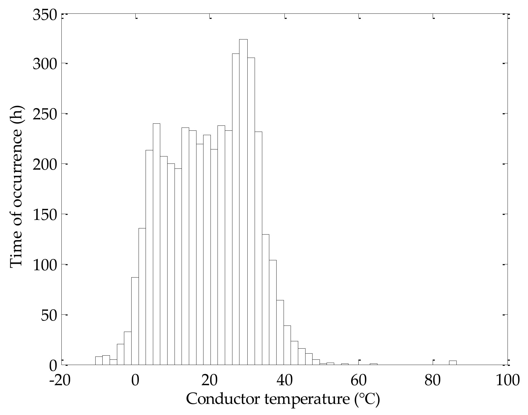
For the transmission line under operation, its carrying current and the meteorological conditions will vary with time and space, and this situation will inevitably lead to time–space variation of conductor temperature. In this paper, the temperature of a LGJ-400/50 conductor (HuaLun Cable, Weihai, China) is calculated by using the wind speed and the ambient temperature data collected over 8784 h in 2016. The maximum allowed current of the LGJ-400/50 conductor is 592 A. The data were measured in Shandong University (Weihai). Assuming the conductor current is 75% of the maximum allowed current, in the above meteorological conditions, the variations and distribution of the conductor temperature for the whole year can be obtained by the CIGRE standard heat balance equation. As shown in Figure 1, the maximum and minimum temperatures are 86.45 °C and −10.79 °C, respectively, and the average temperature is 19.71 °C. The maximum, minimum, and average values of conductor temperature in spring, summer, autumn, and winter are shown in

Table 1. Conductor temperatures in different seasons.

Season	Maximum Value (°C)	Minimum Value (°C)	Average Value (°C)
Spring	56.46	2.50	19.27
Summer	86.45	19.56	32.26
Autumn	53.00	−0.62	21.36
Winter	21.84	−10.79	5.81

.

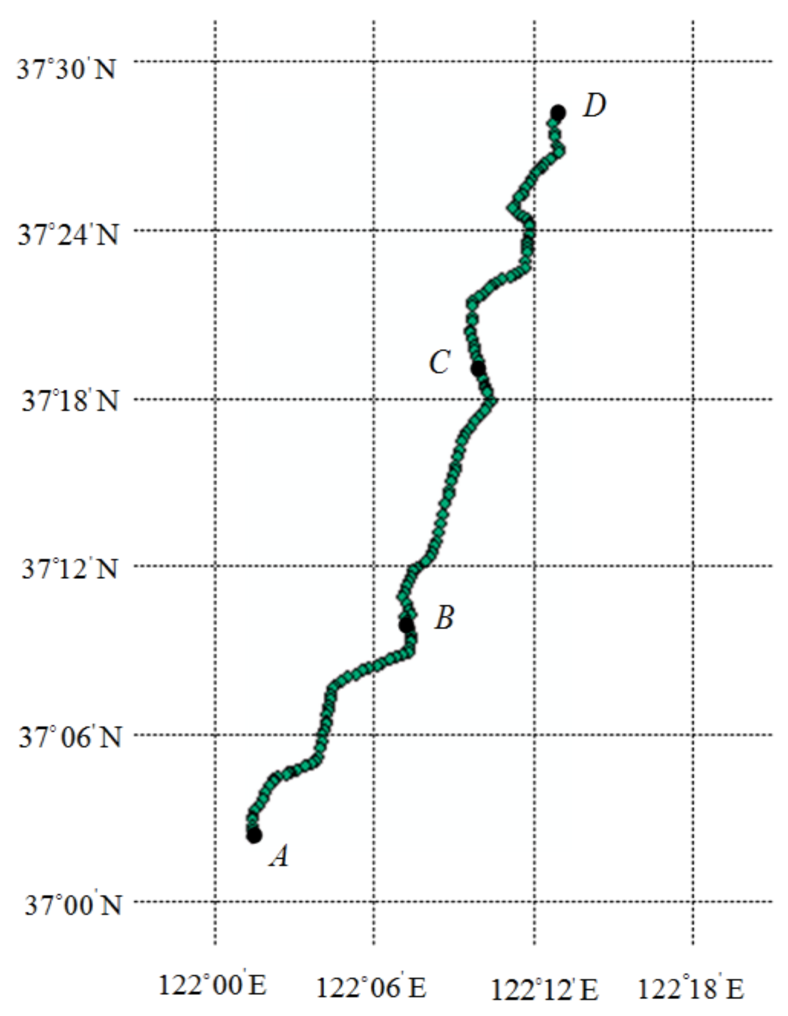
Spatial differences occur in the actual meteorological environment, which can lead to the nonuniform spatial distribution of conductor temperature. For a transmission line with the voltage level of 220 kV, its transmission distance can reach more than 100 km; for a transmission line with the voltage level of 500 kV, its transmission distance can reach 250 km–850 km. The voltage level of the line is 220 kV and its length is 47 km from Weihai to Wendeng. According to the latitude and longitude coordinates of the 148 towers in the line, the geographical orientation of the line is obtained as shown in Figure 2.

In this paper, the GRAPES forecast model produced by the China Meteorological Network is used. The model has the spatial resolution of 10 km and the time resolution of 3 h. In Figure 2, there are 24 intersections of the corresponding longitude and latitude, which are the numerical forecast points for the weather forecast product; and A, B, C, and D are four points on the transmission line which are equally distributed along the latitude. With the abovementioned 24 intersections, the inverse distance interpolation technique is used to obtain the ambient temperature and wind speed at the four points of A, B, C, and D. The inverse distance interpolation technique obtains the parameter value of the estimated point by the linear weighting of known points. The weight coefficient is inversely proportional to the distance.

Table 2. Conductor temperatures at different locations.

Location	Ambient Temperature (°C)	Wind Speed (m/s)	Conductor Temperature (°C)
A	23.47	0.19	54.87
B	23.36	0.35	48.80
C	23.06	0.62	43.32
D	23.54	0.97	40.46

shows the ambient temperature and wind speed at points A, B, C and D on the transmission line at 0:00 on 6 July 2016. Assuming that the current flowing through the conductor is 75% of the maximum allowable current, the conductor temperature at the above four measurement points can be obtained by Equation (2). As shown in Table 2, the conductor temperature difference between the two ends of the transmission line is 14.41 °C.

An example of the variation of the conductor temperature of the transmission line is given above. In this case, the time–space variation of the conductor temperature is obvious. This will result in the time–space variation of the transmission line parameters. The change of line parameters will affect the power flow of the whole system.

4. Relationship between Temperature and Line Parameters

Overhead transmission lines usually have four distributed electrical parameters that affect the head-to-end power transmission, which are series resistance, series inductance, shunt capacitance, and shunt conductance [19,20]. These parameters are mainly determined by the characteristics of conductor materials; the characteristics of the electric and magnetic fields based on the conductor geometry can also determine these parameters. The conductor resistance is related to the conductor temperature, and the relationship is shown in Equation (3):

$$r(T)=r(T_0)·[1+\alpha (T-T_0)]$$

(3)

where $T_0$ is the reference temperature (°C), usually taken as 20 °C; $T$ is the actual temperature of the conductor (°C); $r(T_0)$ is the resistance value at the reference temperature ($\Omega$); $r(T)$ is the resistance at the actual temperature ($\Omega$); and $\alpha$ is the temperature coefficient of resistance (1/°C), which depends on the physical material of the conductor [21,22]. The reactance value of the conductor is also related to the conductor temperature, and the relationship is shown in Equation (4):

$$x_{\mathrm{L}}(T)=x_{\mathrm{L}}(T_0)·[1+\beta (T-T_0)]$$

(4)

where $x_{\mathrm{L}}(T_0)$ is the conductor reactance at the temperature of $T_0$, $x_{\mathrm{L}}(T)$ is the reactance at the temperature of $T$, and $\beta$ is the reactance temperature coefficient.

5. Transmission Line Models Incorporating Conductor Temperature Variation

As mentioned above, the conductor temperature has significant time–space variation characteristics, and the transmission line parameters are related to the conductor temperature. In this paper, the transmission line models considering the variation of conductor temperature are given.

The weather condition and the load are seasonal, which will inevitably lead to seasonal variation of conductor temperature. In this paper, in order to analyze the influence of the change of conductor temperature on the system state, the conductor temperature in different seasons is assumed according to temperatures in Table 1. The conductor temperature $T_{\mathrm{sa}}$ in the spring and autumn is 20 °C, which is always taken as the conductor temperature of the power system. The conductor temperature $T_{\mathrm{sum}}$ in summer is 70 °C, which is taken as the conductor’s maximum permissible operating temperature. According to the actual climate characteristics in Weihai, the conductor temperature $T_{\mathrm{win}}$ in winter is taken as −10 °C. Both meteorological conditions and transmission line parameters have spatial distribution characteristics. In [16], considering that the conductor temperature distribution along the line is not uniform, the conductor temperature of the line can be determined by:

(1) $T_{\mathrm{avg}}$: the average temperature based on the measurement values of the beginning temperature $T_{\mathrm{beg}}$ and the end temperature $T_{\mathrm{end}}$, as shown in Equation (5):

$$T_{\mathrm{avg}}=\frac{T_{\mathrm{beg}}+T_{\mathrm{end}}}{2}$$

(5)

(2) $T_{\mathrm{wavg}}$: the conductor’s weighted average temperature, which is based on the weighted values of the conductor temperature measurement points location on the transmission line, as shown in Equation (6):

$$T_{\mathrm{wavg}}={\displaystyle \sum _{a=1}^{N-1}[(\frac{T_a+T_{a+1}}{2}})\times \frac{\Delta x_{a,a+1}}{l}]$$

(6)

where $N$ is the total number of temperature measurement points, $a$ is a measurement point on the line, $T$ is the temperature of point $a$, $\Delta x_{a,a+1}$ is the line length between point $a$ and its next measurement point $a+1$, and $l$ is the total length of the line.

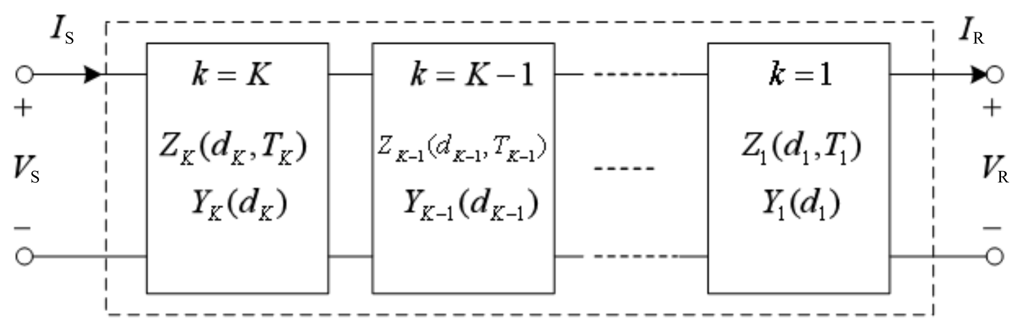
(3) A multisegment transmission line model: the model used in the transmission line can be divided into the $\mathsf{\Pi }$-type or the T-type single segment lumped parameter model. The parameters are calculated at a fixed temperature, and it is clear that it is inconsistent with complex meteorological conditions. The single segment lumped parameter model has difficulty dealing with the nonuniformity of the distribution of conductor temperature along the line. In this paper, in order to evaluate the operating state of the power grid more accurately, we will adopt the multisegment transmission line model based on the spatial distribution of conductor temperature. In [15], the multisegment parameter model of transmission line is given, as shown in Figure 3.

As shown in Figure 3, the state equation of the two-port network of the transmission line is shown by Equation (7):

$$\left[\begin{array}{l}{V}_{\mathrm{R}}\\ I_{\mathrm{R}}\end{array}\right]=\left[\begin{array}{l}1-Z_1\\ -Y_{1}1+Y_1{Z}_1\end{array}\right]\left[\begin{array}{l}1-Z_2\\ -Y_{2}1+Y_2{Z}_2\end{array}\right]\cdots \left[\begin{array}{l}1-Z_k\\ -Y_{k}1+Y_k{Z}_k\end{array}\right]\left[\begin{array}{l}{V}_{\mathrm{S}}\\ I_{\mathrm{S}}\end{array}\right]$$

(7)

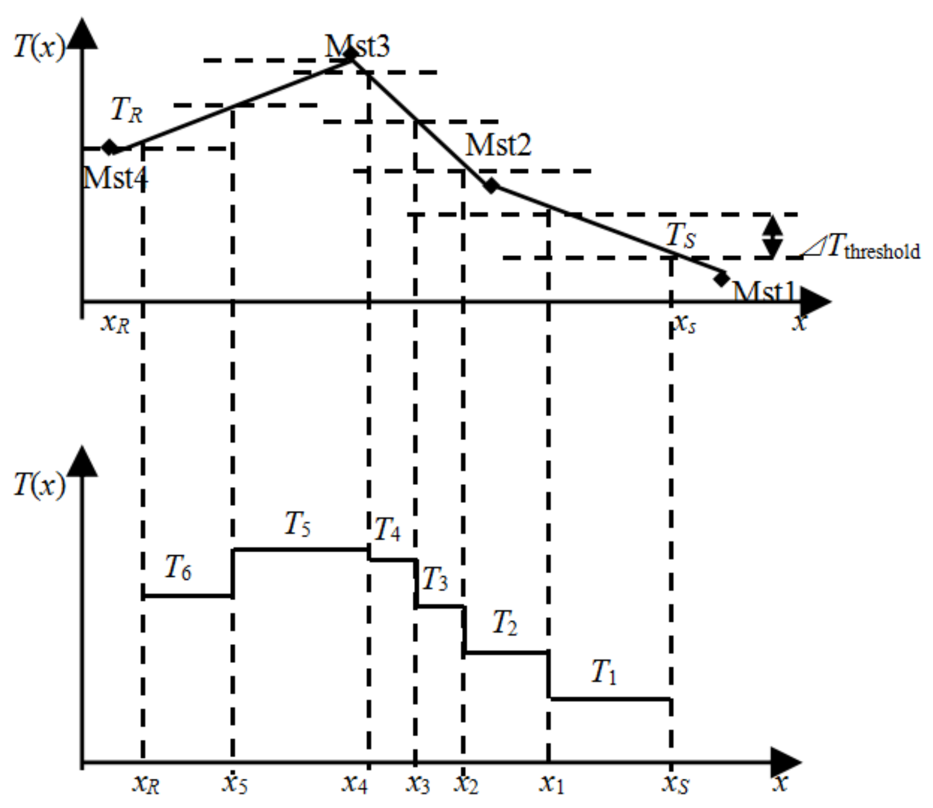
For conductor temperature distribution, as shown in Figure 4, Mst marks the position of the temperature measurement device. The segmentation method of the line is shown as follows:

(1)

Based on the measurement temperature values at the four positions of Mst1, Mst2, Mst3, and Mst4, it is assumed that the distribution of the temperature along the distance x is linear between any two measurement positions, which can enable determination of the temperature distribution between these measurement points. In [15], temperature distribution under the multisegment transmission line model is presented, as shown in Figure 4. If the line sending end $x_{\mathrm{S}}$ and the receiving end $x_{\mathrm{R}}$ are not the location of the temperature measurement device, the temperature values $T_{\mathrm{S}}$ and $T_{\mathrm{R}}$ at the sending end $x_S$ and the receiving end $x_{\mathrm{R}}$, respectively, can be determined by the temperature linear distribution between the measurement points.

(2)

If the allowed maximum temperature difference $\Delta T_{\mathrm{threshold}}$ in any segment has been determined, starting from the line sending point $x_{\mathrm{S}}$, when the temperature difference reaches $\Delta T_{\mathrm{threshold}}$, $x_1$ can be determined. The distance between $x_{\mathrm{S}}$ and $x_1$ is the first segment of the transmission line. The conductor temperature of the first segment $T_1$ is the average of $T(x)$ in this segment. Using this method, we can gradually determine the distance and the temperature values of each segment.

6. Grid Power Flow Involving Conductor Temperature Variation

Assuming that the buses at both ends of a transmission line or a segment are i and j, ignoring the susceptance, the line active and reactive power flow are shown by Equation (8):

$$\begin{array}{l}{P}_{ij}=V_i^2{g}_{ij}(T_l)-V_i{V}_j[g_{ij}(T_l)\cos {\delta }_{ij}-b_{ij}(T_l)\sin {\delta }_{ij}]\\ Q_{ij}=V_i^2{b}_{ij}(T_l)-V_i{V}_j[g_{ij}(T_l)\sin {\delta }_{ij}+b_{ij}(T_l)\cos {\delta }_{ij}]\end{array}$$

(8)

The current flowing through the transmission line or the segment is shown by Equation (9):

$$I_{ij}=\frac{\sqrt{P_{ij}^2+Q_{ij}^2}}{V_i}$$

(9)

where $T_l$ is the conductor temperature of the transmission line l or the segment l; $V_i$ and $V_j$ are the voltage amplitude of bus i and bus j; ${\delta }_{ij}={\delta }_i-{\delta }_j$ is the voltage phase angle difference between bus i and bus j; $g_{ij}$ and $b_{ij}$ are admittance parameters equivalent to the impedance of the transmission line; $g_{ij}=r_{ij}/(r_{ij}^2+x_{ij}^2)$ and $b_{ij}=-x_{ij}/(r_{ij}^2+x_{ij}^2)$ are related to the conductor temperature $T_l$ of the transmission line. When the power system is in operation, the current of the power supply flows into the load through the transmission and distribution components, such as lines and transformers, and the power flow equation of the system is shown by Equation (10):

$$\begin{array}{l}{P}_{\mathrm{G}i}-P_{\mathrm{L}i}={\displaystyle \sum _{j\in i}{P}_{ij}}(V_i,V_j,{\delta }_{ij},T_l)\\ Q_{\mathrm{G}i}-Q_{\mathrm{L}i}={\displaystyle \sum _{j\in i}{Q}_{ij}(V_i,V_j,{\delta }_{ij},T_l)}\end{array}$$

(10)

where $P_{\mathrm{G}i}$ is the input power of the power supply for bus i and $P_{\mathrm{L}i}$ is the load of bus i. $j\in i$ represents that bus j is directly connected to bus i, but bus i is not included. It can be seen from Equation (10) that the change of the conductor temperature of the transmission line will directly lead to the change of the system power flow. The conductor temperature can also be calculated by the steady state heat equation described in Section 2. The heat balance equation and the power flow are two subprograms. When the conductor temperatures of Equation (2) are calculated, Equation (2) receives the carrying currents calculated by Equation (9). When the carrying currents of Equation (9) are calculated, Equation (9) receives the conductor temperatures calculated by Equation (2). The process is solved repeatedly until convergence. The data of the two subprograms are independent of each other, and the appropriate iterative algorithms and the convergence accuracy are adopted respectively. The power flow calculation involving the conductor temperature will be more consistent with the actual operating state of the system.

7. Analysis of Examples

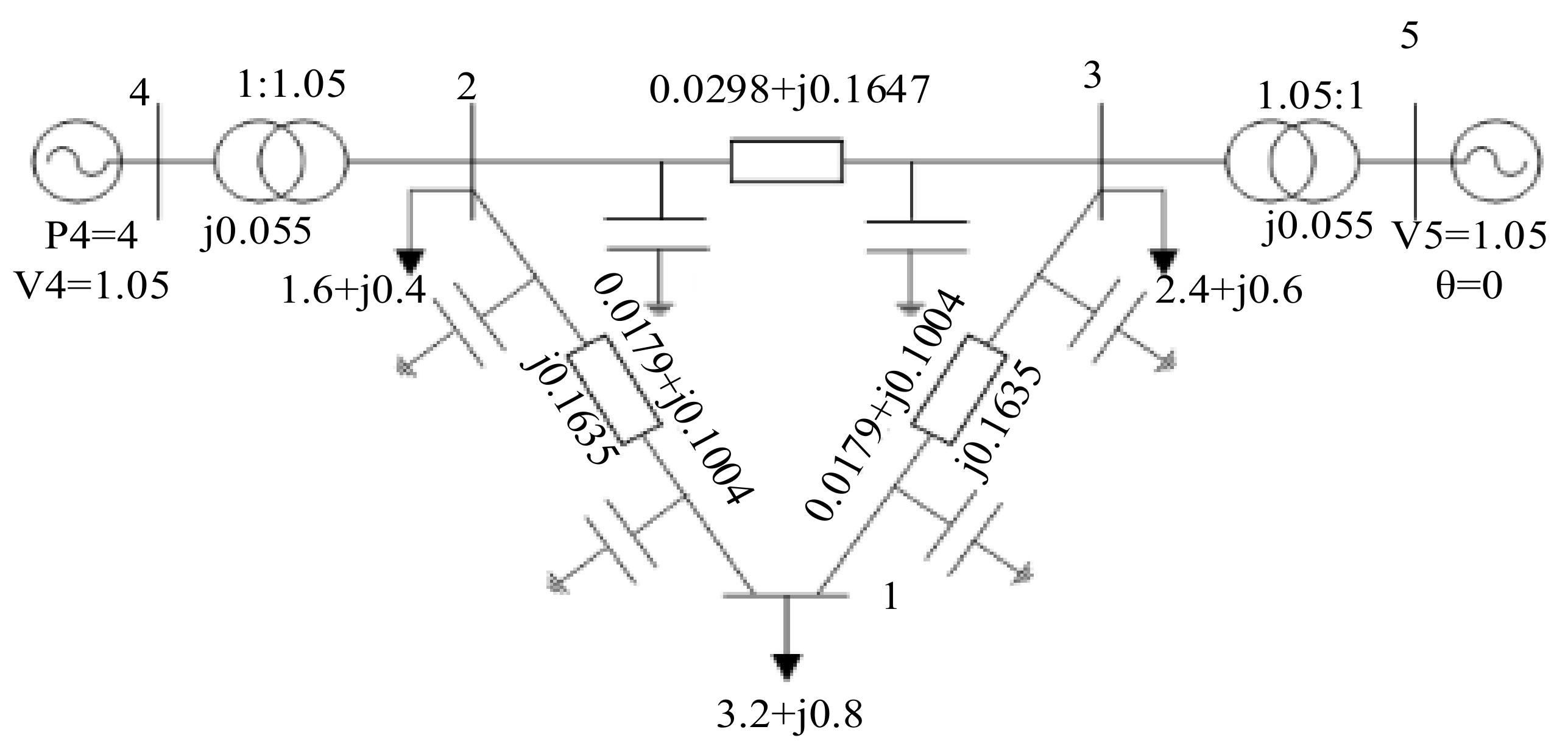
In this paper, an improved five-bus power system is taken as example to analyze the influence of the different temperature models on the system state. The network structure is shown in Figure 5. The voltage level is 220 kV, and the transmission line type is LGJ-400/50, whose section area of aluminum is 399.73 mm². The conductor diameter is 27.63 mm. In the system, the lengths of the branches from points 2-3, 3-1 and 2-1 are 200 km, 120 km, and 120 km, respectively. The coefficient temperature of resistance and reactance of the line is 0.0039 (1/°C).

In order to explain the influence of transmission line temperature on system operation, such as the system power flow and the network loss, the time–space variation of conductor temperature in transmission lines is analyzed and calculated according to the following six cases.

First, the conductor temperatures of all transmission lines in the network of Figure 5 are shown by seasonal temperature values, which correspond to the following three cases, respectively.

Base case: the conductor temperatures of all transmission lines in spring and fall are 20 °C. The line resistance and reactance parameters can be obtained from the manuals, as shown in

Table 3. The impedance and susceptance when the conductor temperature is 20 °C. r: resistance. x: reactance. b: susceptance. p.u.: per-unit value. Branch 2-1: the line from bus 2 to bus 1. Branch 3-1: the line from bus 3 to bus 1. Branch 2-3: the line from bus 2 to bus 3.

Branch	Temperature (°C)	r (p.u.)	x (p.u.)	b (p.u.)
2-1	20	0.0179	0.1004	0.1635
3-1	20	0.0179	0.1004	0.1635
2-3	20	0.0298	0.1674	0.2997

. These are the line parameters used in the routine analysis and calculation of power systems. For this reason, we take this case as the base case.

Case 1: In the hot summer, the increase in ambient temperature and the decrease in wind speed around the transmission line will cause the conductor temperature to increase. In this paper, the conductor temperature of the transmission line in summer is taken as 70 °C. In this case, the line parameters correspond to the maximum permissible operating temperature of the conductor. The impedance and susceptance when the conductor temperature is 70 °C are shown in

Table 4. The impedance and susceptance when the conductor temperature is 70 °C.

Branch	Temperature (°C)	r (p.u.)	x (p.u.)	b (p.u.)
2-1	70	0.0214	0.12	0.1635
3-1	70	0.0214	0.12	0.1635
2-3	70	0.0356	0.2	0.2997

.

Case 2: In the cold winter, the decrease of ambient temperature and the increase of wind speed in the transmission line will cause the line conductor temperature to decrease. According to analysis in Section 3, the conductor temperature is set to be −10 °C. The impedance and susceptance when the conductor temperature is −10 °C are shown in

Table 5. The impedance and susceptance when the conductor temperature is −10 °C.

Branch	Temperature (°C)	r (p.u.)	x (p.u.)	b (p.u.)
2-1	−10	0.0158	0.0887	0.1635
3-1	−10	0.0158	0.0887	0.1635
2-3	−10	0.0263	0.1478	0.2997

.

Secondly, considering the nonuniform spatial distribution of conductor temperature along the line, the following three cases are set:

Case 3: Considering the spatial distribution of conductor temperature, it is assumed that there is a storm at bus 3 on the basis of case 2. Affected by the storm (ambient temperature −32 °C, wind speed 14 m/s), the conductor temperature near bus 3 is −30 °C, when the line current is 120 A. Such for the conductor temperature of branch 2-3, the beginning temperature near bus 3 is −30 °C and the ending temperature near bus 1 is −10 °C. In this case, the conductor temperature is determined by the average temperature of $T_{\mathrm{avg}}$ as shown by Equation (5). The average temperature of branch 3-1 is −20 °C. Similarly, the average temperature of branch 3-1 is also −20 °C, as shown in

Table 6. The impedance and susceptance in case 3.

Branch	Temperature (°C)	r (p.u.)	x (p.u.)	b (p.u.)
2-1	−10	0.0158	0.0887	0.1635
3-1	−20	0.0151	0.0847	0.1635
2-3	−20	0.0252	0.1413	0.2997

.

Case 4: The temperature at both ends of the line is the same as in case 3. Branch 3-1 and branch 2-3 have two known temperature points; the whole line is divided equally by these points and their temperatures are −28 °C and −34 °C, respectively. In this case, the conductor temperature is taken as the weight average $T_{\mathrm{wavg}}$ as shown by Equation (6). The impedance and susceptance of each branch in case 4 are shown in

Table 7. The impedance and susceptance in case 4.

Branch	Temperature (°C)	r (p.u.)	x (p.u.)	b (p.u.)
2-1	−10	0.0158	0.0887	0.1635
3-1	−27.3	0.0146	0.0819	0.1635
2-3	−27.3	0.0243	0.1365	0.2997

.

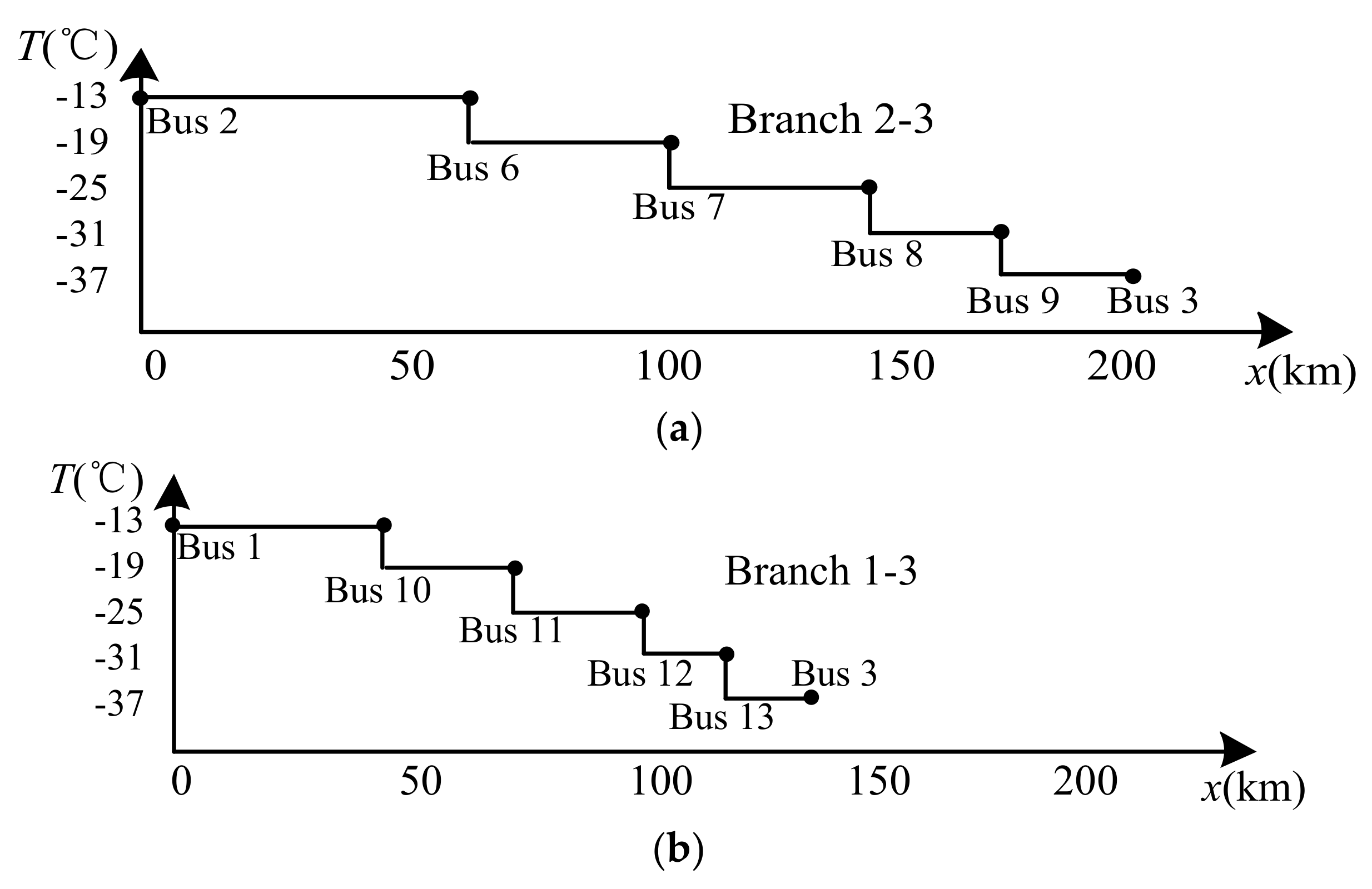
Case 5: The position and temperature information are the same as in case 4; however, the multisegment transmission line model is used. As shown in Figure 6, taking the temperature threshold of 6 °C for segmentation, branches 2-3 and 1-3 can be divided into five segments. Branch 2-3 is divided into segments 2-6, 6-7, 7-8, 8-9, and 9-3; and branch 1-3 is divided into segments 1-10, 10-11, 11-12, 12-13, and 13-3. The segmented system is a 13-bus system, and the operating temperature of each section is the average value of the temperatures at both ends. The temperatures and the values of the series impedance and susceptance of each branch after segmentation are shown in

Table 8. The temperatures and the parameters of each branch after segmentation.

Branch	Beginning Point (km)	End Point (km)	Length (km)	Temperature (°C)	r (p.u.)	x (p.u.)	b (p.u.)
2-1	0.00	120	120	−10	0.0158	0.0887	0.1635
2-6	0.00	22.22	22.22	−13	0.0029	0.0162	0.0333
6-7	22.22	44.44	22.22	−19	0.0028	0.0158	0.0333
7-8	44.44	66.67	22.22	−25	0.0027	0.0153	0.0333
8-9	66.67	133.34	66.67	−31	0.0079	0.0447	0.0999
9-3	133.34	200	66.67	−32	0.0079	0.0445	0.0999
1-10	0.00	13.33	13.33	−13	0.0017	0.0098	0.0182
10-11	13.33	26.67	13.33	−19	0.0017	0.0075	0.0182
11-12	26.67	40	13.33	−25	0.0016	0.0092	0.0182
12-13	40	80	40	−31	0.0048	0.0268	0.0545
13-3	80	120	40	−32	0.0048	0.0267	0.0545

.

7.1. Analysis of Power Flow

The power flow is analyzed according to the above six cases. The calculation results of voltage, current, active power, and system loss are shown in

Table 9. The voltage, active power flow, current, and active power loss of the six cases.

Case	Amplitude V (p.u.)			Phase Angle θ (°)			Power Flow P (MW)			Current I (A)			Active Power Loss (MW)
	1	2	3	1	2	3	2-1	3-1	2-3	2-1	3-1	2-3
Base case	0.9612	1.041	1.035	−16.24	−5.44	−9.19	198.35	132.38	41.65	519.68	359.91	114.96	11.21
Case 1	0.9339	1.0358	1.0298	−18.13	−4.83	−9.32	198.71	134.86	41.29	530	375.14	114.81	14.14
Difference	2.84%	0.5%	0.51%	11.64%	11.21%	1.41%	0.18%	1.87%	0.86%	1.99%	4.23%	0.13%	26.14%
Case 2	0.9758	1.0438	1.038	−15.2	−5.81	−9.12	198.12	131.07	41.88	514.52	352.13	115.06	9.63
Difference	1.52%	0.27%	0.28%	6.4%	6.8%	0.76%	0.12%	0.99%	0.55%	0.99%	2.16%	0.09%	14.09%
Case 3	0.9779	1.0445	1.0379	−15.02	−5.77	−9.11	195.58	133.39	44.42	506.97	357.89	120.53	9.43
Difference	1.74%	0.34%	0.27%	7.51%	6.07%	0.87%	1.4%	0.76%	6.65%	2.45%	0.56%	4.85%	15.88%
Case 4	0.9795	1.0450	1.0379	−14.89	−5.74	−9.11	193.66	135.15	46.34	501.34	362.23	124.70	9.29
Difference	1.90%	0.38%	0.27%	8.31%	5.51%	0.87%	2.36%	2.09%	11.26%	3.53%	0.64%	8.47%	17.13%
Case 5	0.980	1.045	1.038	−14.78	−5.69	−9.11	192.58	136.26	47.45	498.12	379.24	127.01	9.00
Difference	1.96%	0.38%	0.27%	8.99%	4.60%	0.87%	2.91%	2.93%	13.93%	4.15%	5.37%	10.48%	19.71%

. In case 1, it can be seen that the voltage change at bus 1 is maximum compared with the base case. The difference between amplitude of voltage is 2.84% and the difference of phase angle is 11.64%. This is because bus 1 is far from the power supply and the voltage support capability is weak. The differences in the active power flow and the current of branch 3-1 are the maximum, reaching 1.87% and 4.23%, respectively. The difference of active power loss is 26.14% between case 1 and the base case, which is very significant. This is because the resistance parameter of the line is greatly affected by the conductor temperature, and the active power loss of the system is mainly caused by the joule heat generated by the current flowing through the resistance. Compared with case 1, case 2 has a smaller difference in conductor temperature from the base case. As such, the difference of the voltage and the power flow is smaller, but the difference in active power loss still reaches 14.09%.

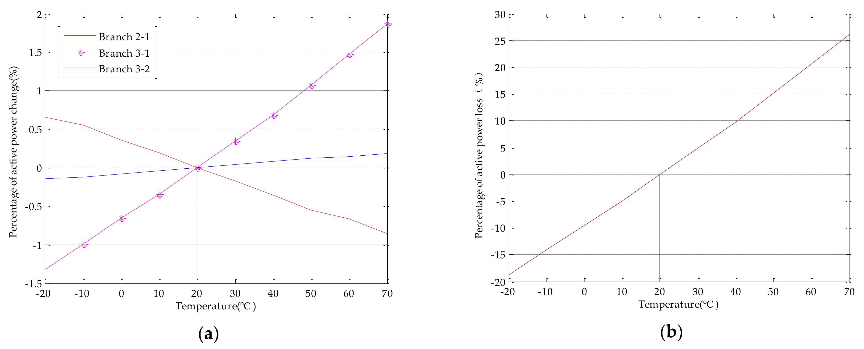
Case 1 and case 2 take into account the seasonal variations of the conductor temperature. Figure 7 shows the variation of the power flow and the system active power loss when the conductor temperatures of the three transmission lines vary from −20 °C to 70 °C. In Figure 7a, the active power flow varies from −0.14% to 0.18% in branch 2-1, from −1.32% to 1.87% in branch 3-1, and from 0.65% to −0.86% in branch 3-2; and in Figure 7b, the system power loss varies from −18.73% to 26.14%. From the above results, it can be seen that the influence of temporal variation of conductor temperature on the system power flow cannot be neglected, especially the influence on the active power loss.

Case 3, case 4, and case 5 not only consider the seasonal variations, but also the nonuniform spatial distribution of conductor temperature based on case 2. The voltage, active power flow, current, and active power loss are shown in Table 9. The results show that the differences between the three cases and the base case are further increased. Among them, the difference between case 5 and the base case is biggest. The maximum differences in voltage and phase angle are 1.96% and 8.99%, respectively. The maximum differences in the power flow and the current are 13.93% and 10.48%, respectively, and the difference of the active power loss is 19.71%. In addition, considering the nonuniform spatial distribution of conductor temperature, different transmission line models are adopted in the three cases. In case 3, the average temperature $T_{\mathrm{avg}}$ of branch 2-3 and 3-1 is −20 °C. In case 4, the weighted average temperature $T_{\mathrm{wavg}}$ along the branch 2-3 and 3-1 is −27.3 °C. The maximum difference of power flow between case 4 and case 3 is 4.32%, the maximum difference of branch current is 3.46%, and the difference of active power loss is 1.48%. Case 5 uses a multisegment transmission line model, and relative to case 3, the maximum differences of power flow, currents, and active power losses are 6.82%, 5.38%, and 4.56%, respectively. From the results, it can be seen that the difference in the system operation state is great when the different transmission line model is adopted. The multisegment transmission line model in case 5 considers the nonuniform spatial distribution of conductor temperature along the transmission line more accurately. The calculation results of the power flow based on this model are more appropriate to the actual operation state of the system.

7.2. Maximum Power Transmission

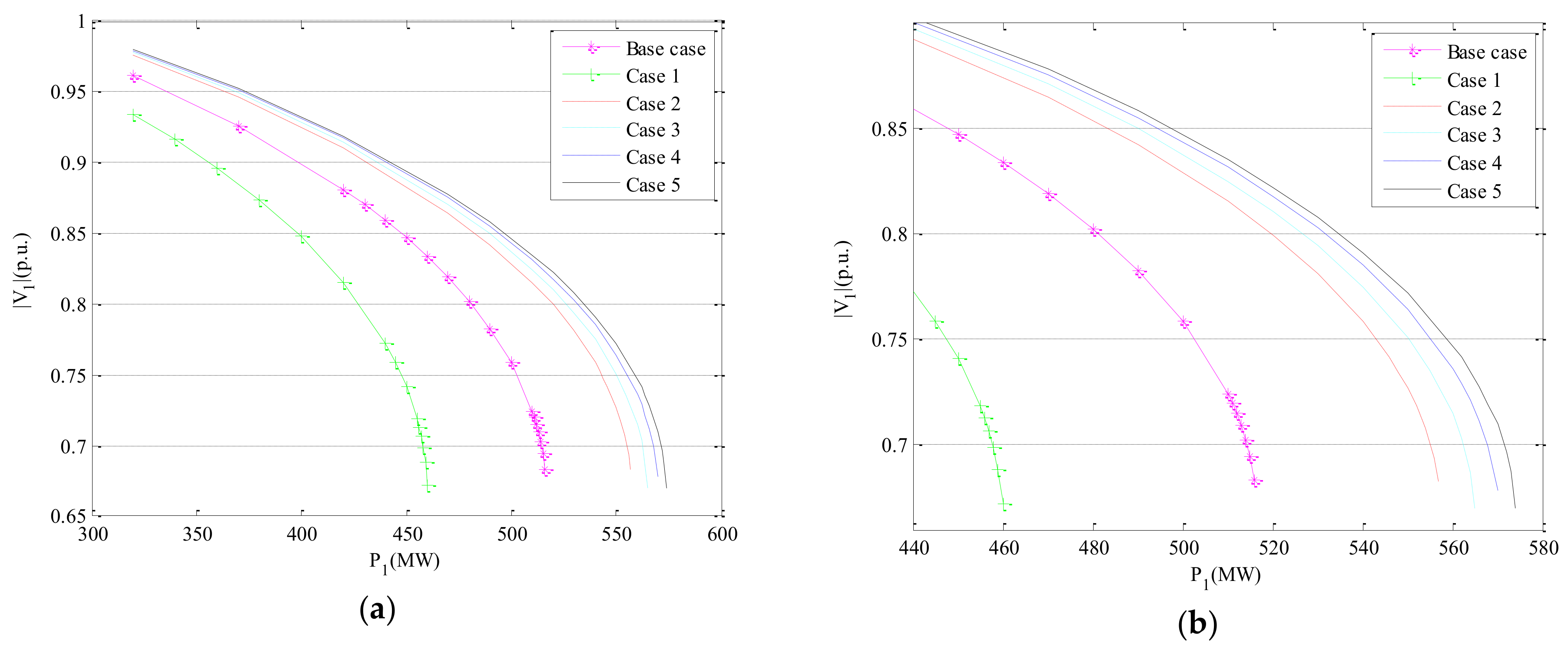
In order to study the influence of the temperature distribution on the transmission capacity of the transmission lines, the active and reactive loads of bus 1 are increased by the same proportion. Figure 8 shows the PV (The Voltage and Power) curves for the six cases. The maximum transmission power and voltage are listed in

Table 10. Maximum power transmission under seasonal variation.

Case	${\mathbf{P}}_1$ (MW)	${\mathbf{V}}_1$ (p.u.)
Base case	516	0.6835
Case 1	460	0.6721
Difference	−10.85%	−1.67%
Case 2	557	0.6828
Difference	7.95%	−0.1%

and

Table 11. Maximum power transmission under spatial variation.

Case	${\mathbf{P}}_1$ (MW)	${\mathbf{V}}_1$ (p.u.)
Case 2	557	0.6828
Case 3	565	0.6704
Difference	1.44%	−1.82%
Case 4	570	0.6785
Difference	2.33%	−0.63%
Case 5	574	0.67
Difference	3.05%	−1.87%

in detail. Table 10 shows the maximum power transmission characteristics of the transmission lines under seasonal variations. The maximum power of the base case is 516 MW and the maximum power of case 1 is 460 MW, which is −10.85% difference from the base case. The maximum power of case 2 is 557 MW, which is 7.95% difference from the base case. It can be seen that the seasonal variations of conductor temperature has a great influence on the maximum power transmission of the lines. This is because the conductor temperature changes will directly lead to the change of the line parameters.

Table 11 shows the maximum power transmission characteristics of the transmission line under the consideration of spatial distribution. Case 3 has a maximum power of 565 MW, with a difference of 1.44% from case 2. Case 4 has a maximum power of 570 MW, with a difference of 2.33% from case 2. Case 5 has a maximum power of 574 MW, with a difference of 3.05% from case 2. These results are consistent with the expected results. In case 5, the segmentation method is used, which is the most appropriate description of the actual situation and has the biggest difference from case 2. With the average temperature, case 3 is closest to the case 2. With the weighted average temperature, case 4 is between case 3 and case 5. The comparison of these three cases and case 2 shows that spatial distribution has a great influence on the maximum power transmission of the lines.

8. Conclusions

If the transmission line is set to a fixed lumped parameter model, the resulting power flow and maximum transmission power of the transmission lines are in great deviation from the actual situation. In this paper, an example is given to verify that the conductor temperature of transmission line has obvious time–space variation characteristics, and it has an important influence on the operation state of the power system. In this paper, a seasonal model considering conductor temperature temporal distribution is established. In addition, considering conductor temperature spatial distribution, the average value model, weighted average value model, and the segmentation model are applied. Based on the above models, the system power flow and the maximum transmission power are analyzed. The calculation results show that it is necessary to consider the time–space distribution of the conductor temperature in the analysis of power system operation, and that the line segmentation model is more suitable for the actual operation of the system. In the future, combined with the dynamic thermal rating, the influence of the weather conditions along the transmission lines, such as ambient temperature, wind speed, and solar radiation intensity, on the system power flow and maximum power transmission will be studied.