The Study of Turbulent Fluctuation Characteristics in a Small Rotary Engine with a Peripheral Port Based on the Improved Delayed Detached Eddy Simulation Shear-Stress Transport (IDDES-SST) Method

Abstract
:1. Introduction
2. Mathematical Model
2.1. Improved Delayed Detached Eddy Simulation (IDDES) Model
2.2. Flow-Field Decomposition
2.3. Velocity Circulation
2.4. Q-Criterion
3. Geometric Model and Dynamic Meshing
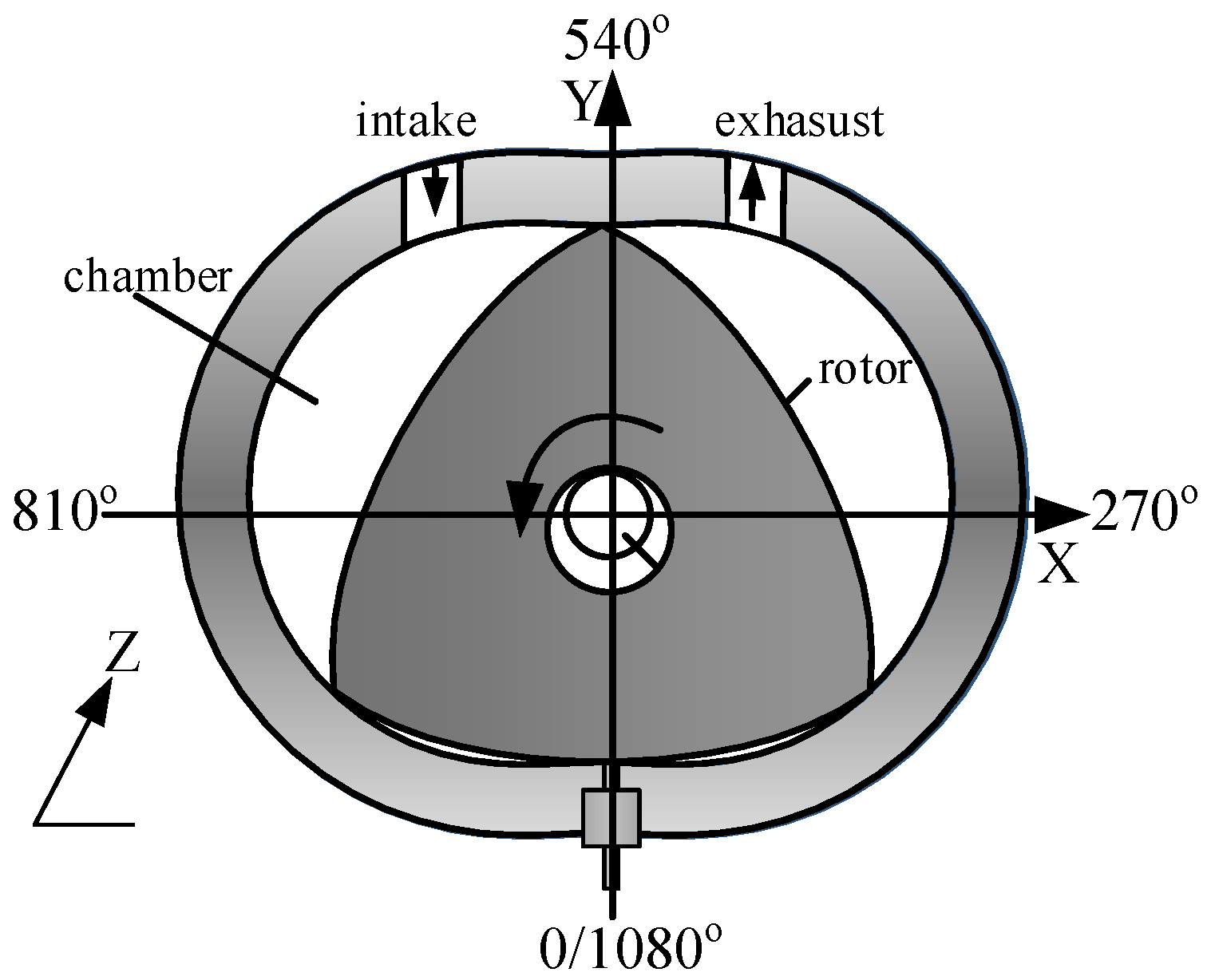
3.1. Geometric Model
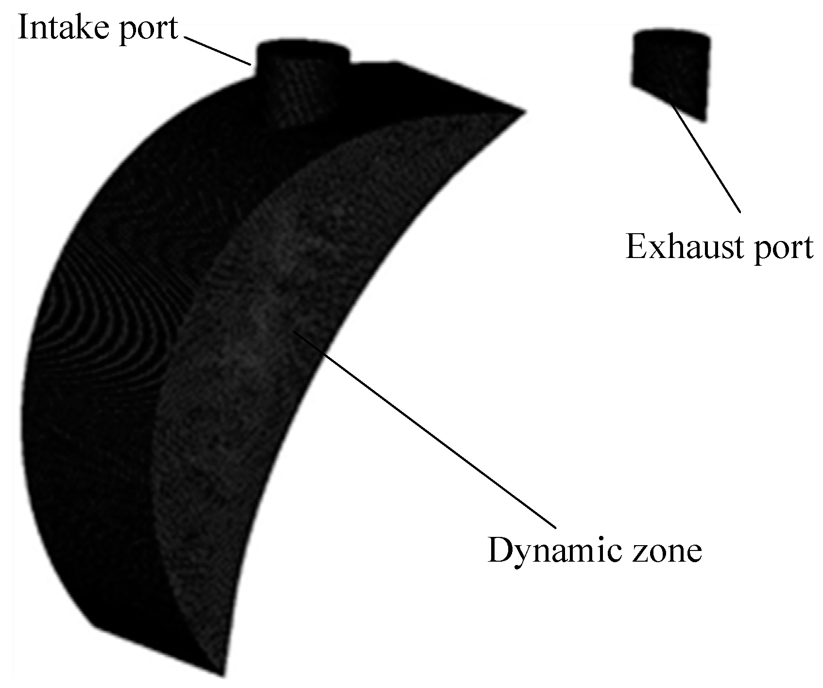
3.2. Dynamic Meshing
4. Boundary Conditions and IDDES Model Validation
4.1. Determination of Time Step Size
4.2. Computing Model and Boundary Condition
4.3. Experimental Results
5. Results and Discussion
5.1. Velocity Field
5.2. Coherent Structure
5.3. Velocity Fluctuation
5.4. Velocity Circulation
6. Conclusions
- (1)
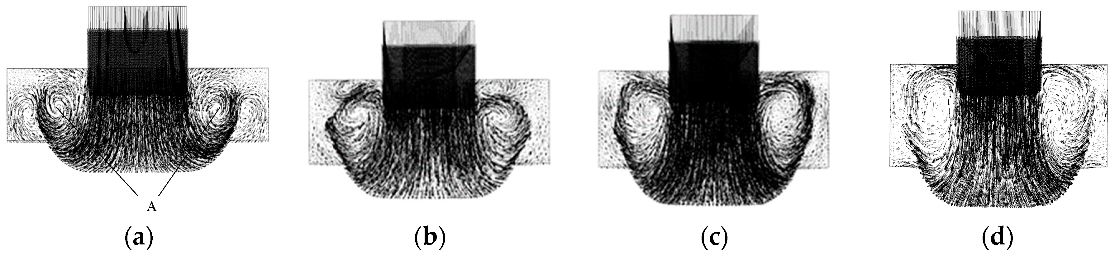
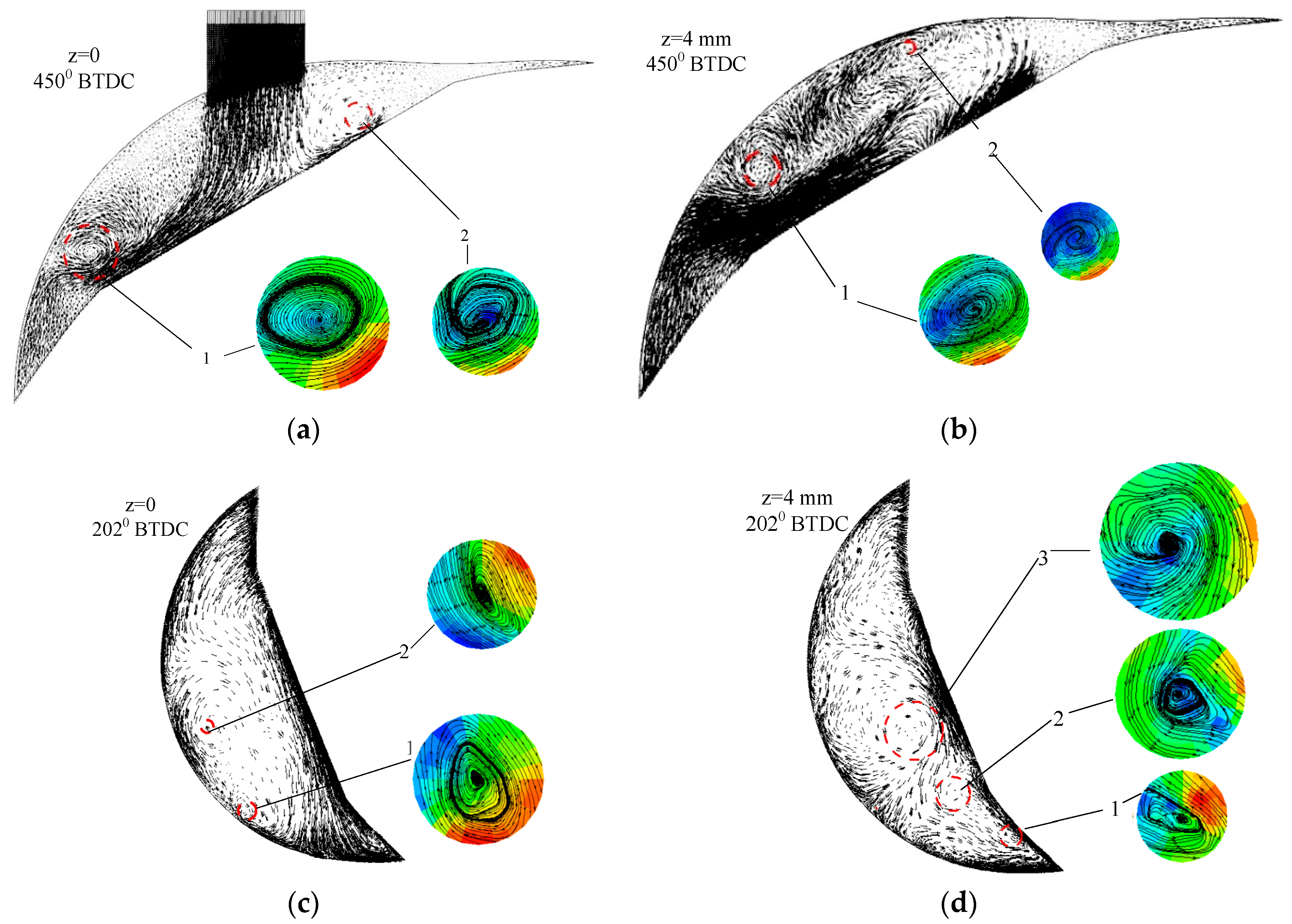
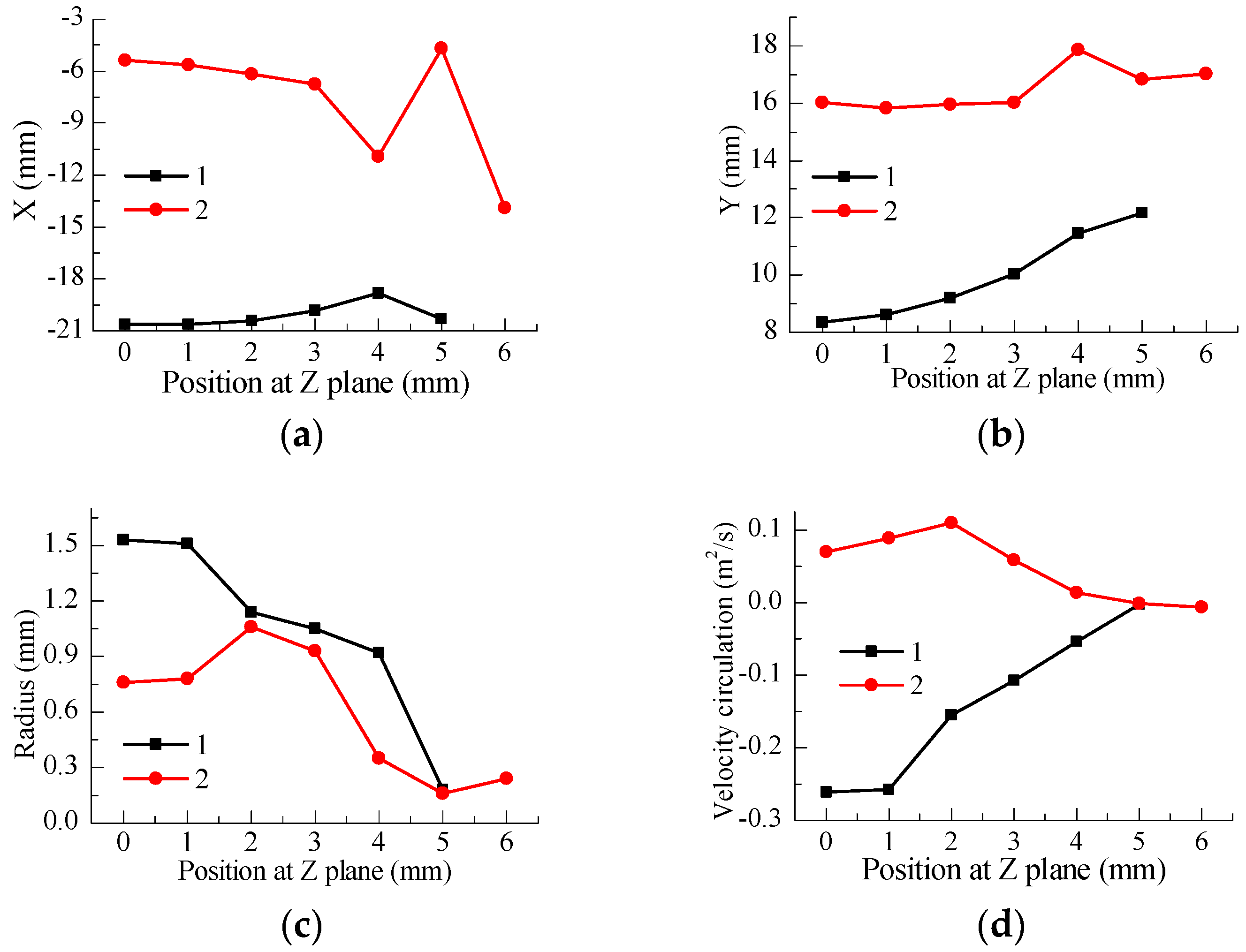
- In the initial phase of the intake stroke, two reverse vortices with the same radius form at one side of the intake port. With the operation of the engine, the radius of the clockwise vortices keeps increasing and several small vortex structures without dominant flow direction occur at different positions.
- (2)
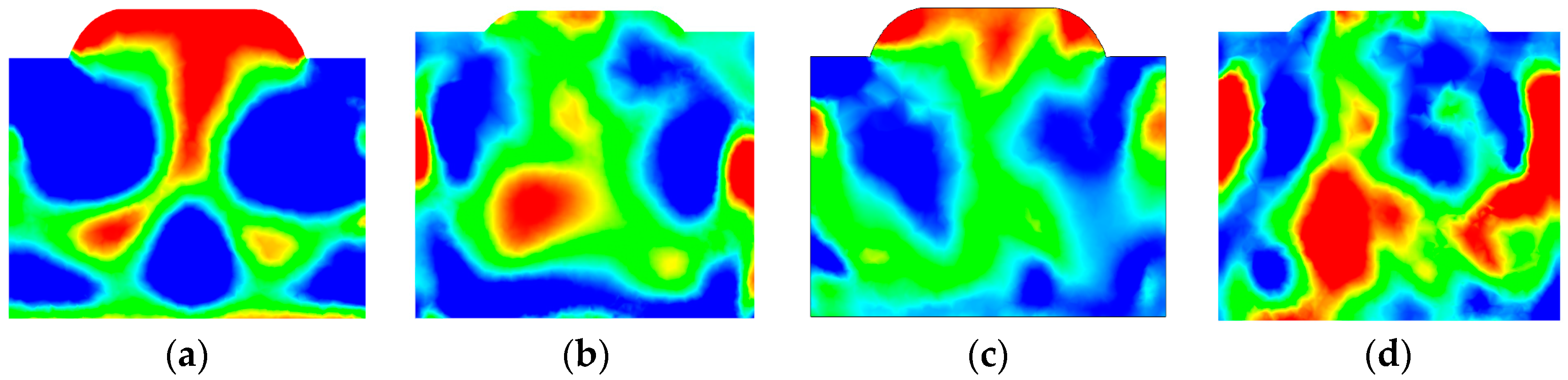
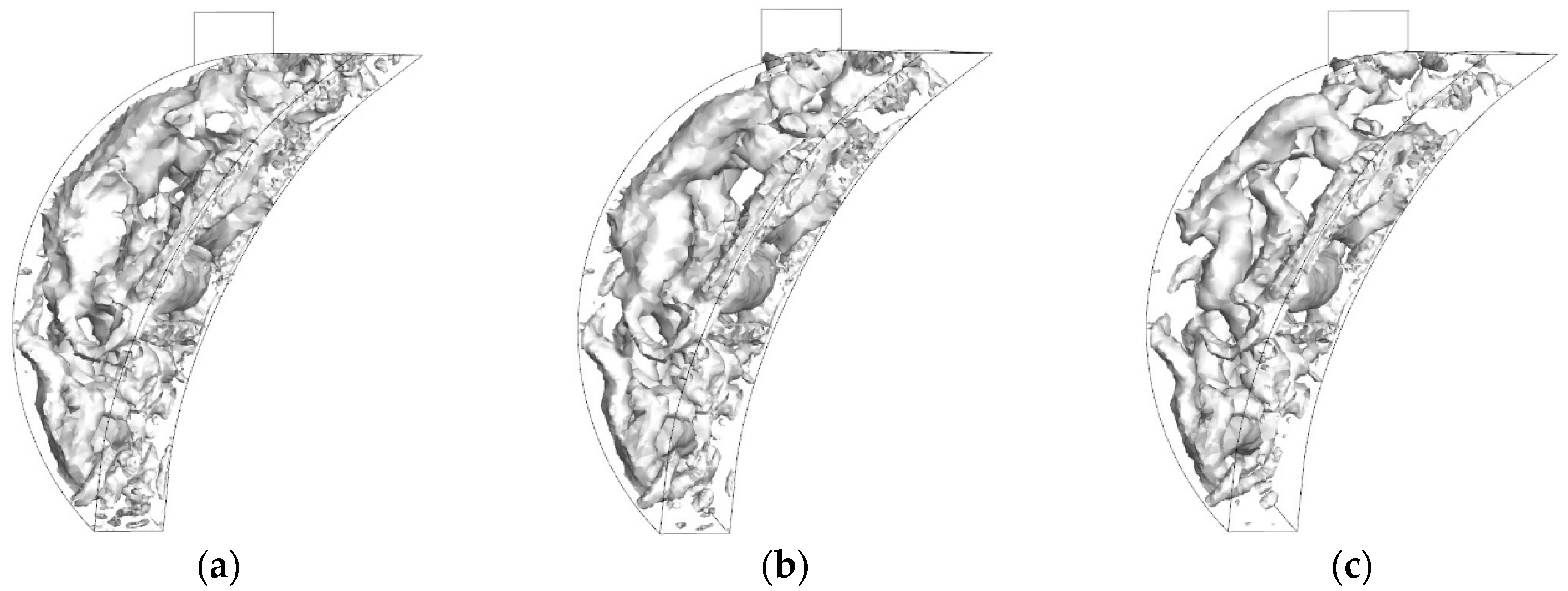
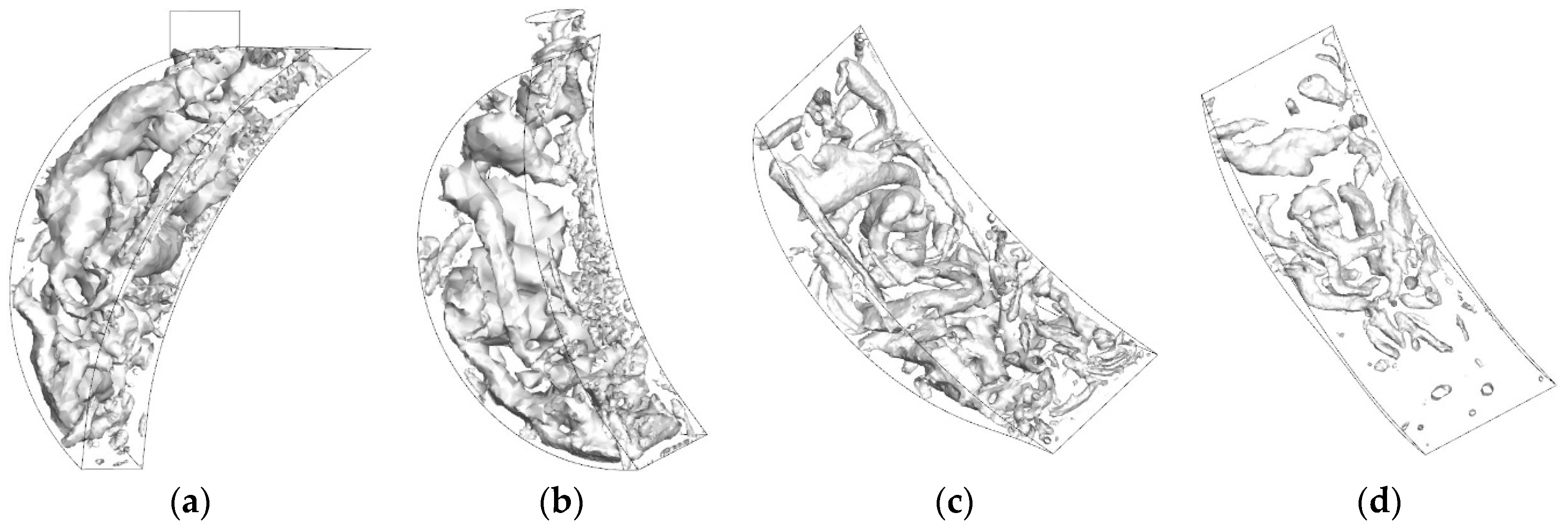
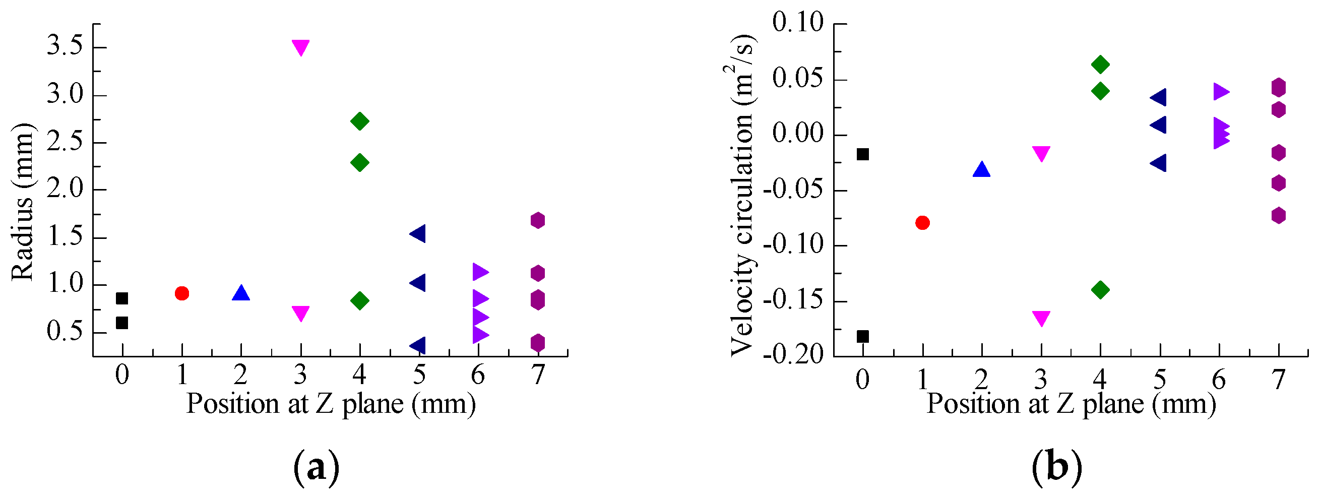
- At 15,000 r/min, the large-scale vortex structures with high intensity mainly gather in the center of the chamber and go through deformation and are broken during the intake process. At 135° BTDC, lots of small vortex structures distribute throughout the whole space of the chamber. Most of the vortices disappear at the end of the compression stroke.
- (3)
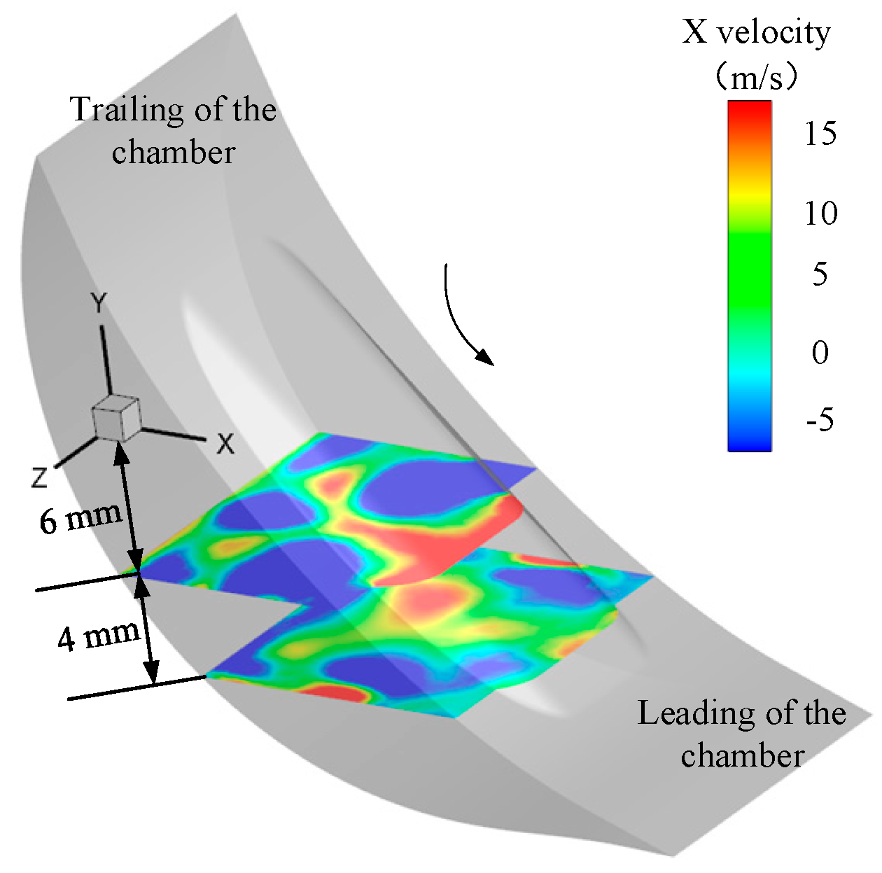
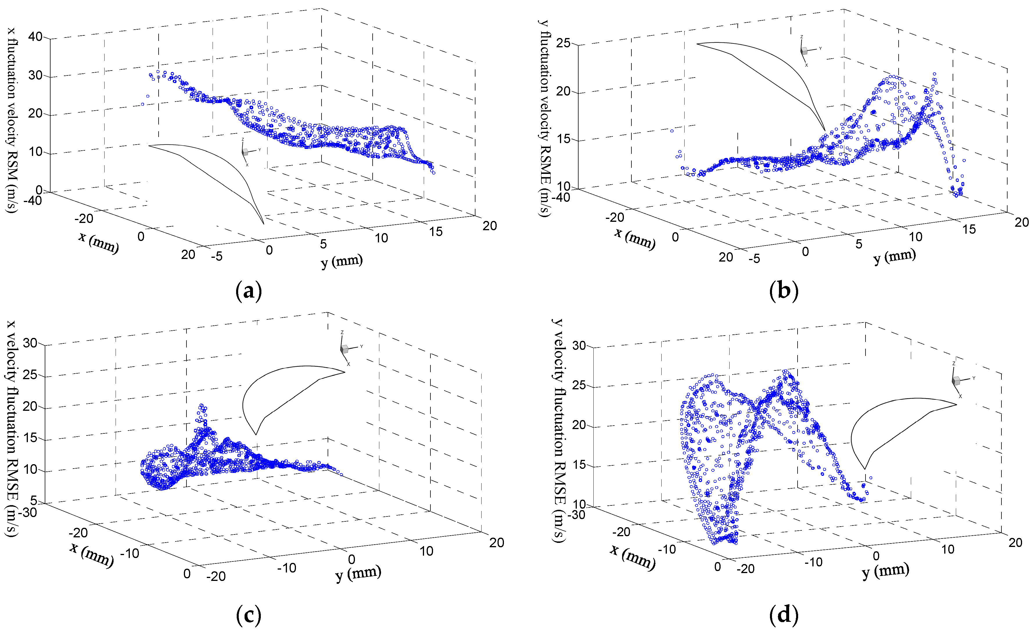
- Flow stability of the X direction increases from the leading to the trailing. The calculated results show the maximum fluctuation velocity RMS at the X direction is mostly four times larger than its minimum at 450° BTDC. The distribution of Y velocity RMS is like a paraboloid and the peak position moves from the mid-back to the middle of the chamber.
- (4)
- In the intake phase, two vortices occur at the cross section parallel to the covers and are located at the leading and trailing of the cross section, respectively. Compared to the intake process, more vortices occur at cross sections which are far away from the central section during the compression process.
Author Contributions
Conflicts of Interest
Nomenclature
| N | cycle number |
| mean velocity | |
| transient fluctuation velocity | |
| fluctuation velocity | |
| velocity circulation | |
| fluctuation velocity magnitude at X, Y | |
| X, Y coordinate X, Y coordinate | |
| vorticity | |
| J | vortex intensity |
| mean strain rate tensor | |
| tensor of stress | |
| turbulent kinetic energy | |
| t | time |
| L | a certain close curve |
| IDDES length scale | |
| RANS length scale | |
| LES length scale | |
| grid scale | |
| empirical constant | |
| factor of length scale | |
| distance to the nearest wall | |
| empirical delay function | |
| elevating function | |
| F1 | first blending function of the SST |
| Greek Letters | |
| density | |
| molecular viscosity | |
| turbulent viscosity | |
| blending function | |
| constant value | |
| Acronyms | |
| LES | large eddy simulation |
| RNS | Reynolds-average Navier Stoke |
| LDV | laser doppler velocimetry |
| BTDC | before top dead center |
| ATDC | after top dead center |
| RNG | renormalization group |
| CA | crank angle |
| DES | mean strain rate tensor |
| IDDES | improved delayed detached eddy simulation |
| TKE | turbulent kinetic energy |
| SST | shear-stress transport |
| PIV | particle image velocimetry |
References
- Picard, M.; Tian, T.; Nishino, T. Predicting gas in the rotary engine—Part I: Apex and corner seals. ASME 2016, 138, 1–8. [Google Scholar] [CrossRef]
- Picard, M.; Tian, T.; Nishino, T. Predicting gas in the rotary engine—Part II: Side seals and summary. ASME 2016, 138, 1–8. [Google Scholar] [CrossRef]
- McReynolds. Small engine, an energy perspective. SAE Pap. 1979, 790477. [Google Scholar] [CrossRef]
- Fan, B.W.; Pan, J.F.; Yang, W.M.; An, H.; Tang, A.; Shao, X.; Xue, H. Effects of different parameters on the flow field of peripheral ported rotary engine. Eng. Appl. Comput. Fluid 2015, 9, 445–457. [Google Scholar] [CrossRef]
- Shih, T.I.P.; Schock, H.J.; Nguyen, H.I.; Stegeman, I.D. Numerical simulation of the flow field in a motored two-dimensional Wankel engine. J. Propul. Power 1987, 3, 269–276. [Google Scholar] [CrossRef]
- Fan, B.W.; Pan, J.F.; Pan, Z.H.; Tang, A.K.; Zhu, Y.J.; Xue, H. Effects of pocket shape and ignition slot locations on the combustion processes of a rotary engine fueled with natural gas. Appl. Therm. Eng. 2015, 89, 11–27. [Google Scholar] [CrossRef]
- Fan, B.W.; Pan, J.F.; Tang, A.K.; Pan, Z.H.; Zhu, Y.J.; Xue, H. Experimental and numerical investigation of the fluid flow in a side-ported rotary engine. Energy Convers. Manag. 2015, 95, 385–397. [Google Scholar] [CrossRef]
- Meloni, R.; Naso, V. An Insight into the Effect of Advanced Injection Strategies on Pollutant Emissions of a Heavy-Duty Diesel Engine. Energies 2013, 6, 4331–4351. [Google Scholar] [CrossRef]
- Celik, I.; Yavuz, I.; Smirnov, A. Large eddy simulations of in-cylinder turbulence for internal combustion engines: A review. Int. J. Engine Res. 2001, 2, 119–148. [Google Scholar] [CrossRef]
- Haworth, D.C.; Jansen, K. Large-eddy simulation on unstructured deforming meshes: Towards reciprocating IC engines. Comput. Fluids 2000, 29, 493–524. [Google Scholar] [CrossRef]
- Wang, T.; Zhang, X.; Xu, J.; Zheng, S.Z.; Hou, S.X. Large-eddy simulation of flame-turbulence interaction in a spark ignition engine fueled with methane/hydrogen/carbon dioxide. Energy Convers. Manag. 2015, 104, 147–159. [Google Scholar] [CrossRef]
- Lei, H.; Zhou, D.; Bao, Y.; Li, Y.; Han, Z.L. Three-dimensional Improved Delayed Detached Eddy Simulation of a two-bladed vertical axis wind turbine. Energy Convers. Manag. 2017, 133, 235–248. [Google Scholar] [CrossRef]
- Spalart, P.R.; Jou, W.H.; Strelets, M.; Allmaras, S. Comments on the Feasibility of LES for Wings, and on a Hybrid RANS/LES Approach. In Proceedings of the Advances in DNS/LES, Louisiana Tech University, Ruston, LA, USA, 4–8 August 1997. [Google Scholar]
- Sagaut, P. Large Eddy Simulation for Incompressible Flow: An Introduction, 3rd ed.; Springer: Paris, France, 2006; pp. 83–89. ISBN 3-540-26344-6. [Google Scholar]
- Gritskevich, M.; Garbaruk, A.; Schütz, J.; Menter, F. Development of DDES and IDDES Formulations for the k-ω Shear Stress Transport Model. Flow Turbul. Combust. 2012. [Google Scholar] [CrossRef]
- Menter, F.R.; Kuntz, M.; Langtry, R. Ten years of industrial experience with the SST turbulence model. In Proceedings of the 4th International Symposium on Turbulence Heat and Mass Transfer, Antalya, Turkey, 12–17 October 2003. [Google Scholar]
- Hasse, C.; Sohm, V.; Durst, B. Detached eddy simulation of cyclic large scale fluctuations in a simplified engine setup. Int. J. Heat Fluid Flow 2009, 30, 32–43. [Google Scholar] [CrossRef]
- Hasse, C.; Sohm, V.; Durst, B. Numerical investigation of cyclic variations in gasoline engines using a hybrid URANS/LES modeling approach. Comput. Fluids 2010, 39, 25–48. [Google Scholar] [CrossRef]
- Shur, M.L.; Spalart, P.R.; Strelets, M.K.; Travin, A.K. A hybrid RANS-LES approach with delayed-DES and wall-modelled LES capabilities. Int. J. Heat Fluid Flow 2008, 29, 1638–1649. [Google Scholar] [CrossRef]
- Menter, F.R. Two-equation eddy-viscosity turbulence models for engineering applications. In Proceedings of the AIAA 23rd Fluid Dynamics, Plasma Dynamics, and Lasers Conference, Orlando, FL, USA, 6–9 July 1993; pp. 1598–1605. [Google Scholar]
- Liu, D.M.; Wang, T.Y.; Jia, M.; Wang, G.D. Cycle-to-cycle variation analysis of in-cylinder flow in a gasoline engine with variable valve lift. Exp. Fluids 2012, 53, 585–602. [Google Scholar] [CrossRef]
- Li, Y.; Zhao, H. Characterization of an in-cylinder flow structure in a high-tumble SI engine. Int. J. Engine Res. 2004, 5, 375–400. [Google Scholar] [CrossRef]
- Heinirich, V. Detection of vortices and quantitative evaluation of their main parameters from experimental velocity data. Meas. Sci. Technol. 2001. [Google Scholar] [CrossRef]
- Hunt, J.C.R.; Wray, A.; Moin, P. Eddies, stream and convergence zones in turbulent flows. In Proceedings of the Center for Turbulence Research Proceedings of the Summer Program, NASA, Stanford University, Stanford, CA, USA, 1 December 1988. [Google Scholar]
- DeFilippis, M.; Hamady, F.; Novak, M.; Schock, H. Effects of pocket configuration on the flow field in a rotary engine assembly. SAE Pap. 1992, 920300. [Google Scholar] [CrossRef]

| Parameter | Value |
|---|---|
| Generating radius | 21 mm |
| Eccentricity | 3 mm |
| Displacement | 5 mL |
| Compression ratio | 8.5 |
| Width | 14.5 mm |
| Intake phase | Advanced angle, 459° BTDC; Delay angle, 220° ATDC |
| Exhaust phase | Advanced angle, 198° BTDC; Delay angle, 486° ATDC |
| CA/° | Experimental Results | Simulation Results |
|---|---|---|
| 730 | 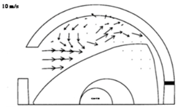 | 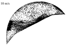 |
| 820 | 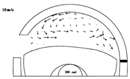 |  |
| 910 | 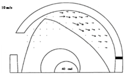 |  |
| 1000 |  |  |
© 2018 by the authors. Licensee MDPI, Basel, Switzerland. This article is an open access article distributed under the terms and conditions of the Creative Commons Attribution (CC BY) license (http://creativecommons.org/licenses/by/4.0/).
Share and Cite
Zhang, Y.; Liu, J.; Zuo, Z. The Study of Turbulent Fluctuation Characteristics in a Small Rotary Engine with a Peripheral Port Based on the Improved Delayed Detached Eddy Simulation Shear-Stress Transport (IDDES-SST) Method. Energies 2018, 11, 642. https://doi.org/10.3390/en11030642
Zhang Y, Liu J, Zuo Z. The Study of Turbulent Fluctuation Characteristics in a Small Rotary Engine with a Peripheral Port Based on the Improved Delayed Detached Eddy Simulation Shear-Stress Transport (IDDES-SST) Method. Energies. 2018; 11(3):642. https://doi.org/10.3390/en11030642
Chicago/Turabian StyleZhang, Yan, Jinxiang Liu, and Zhengxing Zuo. 2018. "The Study of Turbulent Fluctuation Characteristics in a Small Rotary Engine with a Peripheral Port Based on the Improved Delayed Detached Eddy Simulation Shear-Stress Transport (IDDES-SST) Method" Energies 11, no. 3: 642. https://doi.org/10.3390/en11030642
APA StyleZhang, Y., Liu, J., & Zuo, Z. (2018). The Study of Turbulent Fluctuation Characteristics in a Small Rotary Engine with a Peripheral Port Based on the Improved Delayed Detached Eddy Simulation Shear-Stress Transport (IDDES-SST) Method. Energies, 11(3), 642. https://doi.org/10.3390/en11030642