A Hysteresis Model for Fixed and Sun Tracking Solar PV Power Generation Systems

Abstract

In this study, a new solar photovoltaic (PV) panel output power model is proposed. The model is constructed as a function of ambient temperature and solar radiations for two types (fixed panel and sun tracking panel) of PV systems. The proposed models are tested and verified on the Renewable Energy Research Home (RERH) system that was installed at the Anadolu University campus in Eskişehir, Turkey. The model is deliberately constructed for the winter season, where cloudliness, rain and snow constitute more challenging conditions for modeling. The developed model outcomes are compared to the outputs of state of the art methods that use global solar radiation and temperature data. A total of eight algebraic models are constructed for the purpose of depicting the solar radiation-to-electric power behavior. It is observed that even the least successful one of these eight variants are performing better than the most accurate method in the literature. It is argued that mathematical incorporation of the proposed novel hysteresis functions to the solar radiation-to-power conversion curves results in a richer class of functions and causes a significant accuracy improvement on the mathematical power generation model, even for the most challenging season of winter.

1. Introduction

Alternative energy sources are of great importance in the world in order to reduce hydrocarbon dependency in electricity generation. Being a sustainable, emission-free and cost effective source, the share of solar energy inside the overall electricity generation is rapidly increasing. PV systems have become widespread in recent years [1]. In order to use the solar energy sources reliably in grid operations, it is important to forecast accurately the total electricity generated from the PV system in order to realize planning of a PV system under different environmental conditions. With an accurate estimation of the total power generated from the solar system, it is possible to perform efficient energy analysis in order to meet the required energy demand. Consequently, it becomes possible to help grid operators manage the power balance between electricity demand and supply. Especially in applications such as optimum bidding [2] and sizing of energy storage [3] for microgrids, the accurate maximum power output of solar PV panels are required. In the literature, different studies have been carried out regarding the estimation methods for solar electricity generation. In general, these methods are divided into three basic groups as (i) physical; (ii) statistical and (iii) hybrid methods [4]. Physical models use global solar radiation, ambient temperature, relative humidity and some other outdoor weather parameters [5,6]; statistical techniques use past recorded data to model linear time series via related characteristics of the past days [7,8,9]. Hybrid models were developed to combine two or more models in order to avoid the disadvantages of a single model [10,11,12]. Some heuristic approaches based on artificial intelligence were also applied to forecast energy generation successfully [13,14,15,16,17,18]. The most commonly used (and accepted as state of the art in several applications) maximum power output model uses global solar radiation and ambient temperature values as input parameters to the forecasting function [2,3,19,20]. The expected global solar radiation value on PV panels at a certain time can be calculated/estimated by the locations and orientations of the panels [5]. However, due to the high uncertainty on the variation of climatic conditions in any specified region, it is quite difficult to predict the solar radiation on PV panels. Several attempts exist for forecasting global solar radiation [21,22,23,24,25,26,27,28,29,30,31].

The efficiency of PV panels and the unavoidable system losses directly affect the power output. Unfortunately, losses and efficiency of the overall system are not static. Unavoidably, they deteriorate in the long run by aging. More importantly, they show shorter performance variations due to changing ambient temperatures. PV panels’ current-voltage (I-V) curves depend on both solar radiation and temperature [32]. It is also reported that panel electricity generation depends on whether parameters such as humidity, wind speed/direction, etc. [33]. These parameters are naturally time varying and have nonlinear relations to output power values. Even if global solar radiation and temperature values are known, the used output power model in [3] for PV panels is insufficient when compared with real measurements. In our previous study [34], we observed that a certain solar radiation value causes the generation of different electric power values depending on whether the same radiation value appears in the morning or in the afternoon. In [34] we propose that this difference in the morning and afternoon radiation-to-power generation efficiencies can be modeled as a piece-wise time-dependent function with three parts (corresponding to morning, noon and afternoon times). In that work, each piece-wise part was modeled a 2nd order function of the solar radiation. According to that model, it was concluded that the global solar radiation-to-energy conversion phenomenon is not only non-linear, but it also has a strong time-varying characteristic. In Section 3, it is illustrated that the solar radiation-to-power conversion function requires a time varying model that exhibits a hysteresis behavior on the conversion curve. In general, the term hysteresis is used for describing systems that exhibit a history-dependent behavior causing a change (usually a lag) in the output of a function to input values. More precisely, hysteresis is defined as “the phenomenon in which the value of a physical property lags behind changes in the effect causing it” [35]. This phenomenon is encountered in a rich class of disciplines, ranging from chemistry to engineering, from biology to even economics [35]. A related hysteresis phenomenon was encountered in solar cells, where an anomalous hysteresis phenomena was observed in the current-voltage curves due to their temperature dependency [36,37]. In this study, the characteristics of the solar radiation-to-power conversion of PV panels are considered. According to the above hysteresis definition [35], the physical property of the system is taken as electric energy (voltaic output) and the “effect causing it” is taken as solar radiation (photons), hence the name of the device: photo-voltaic panel. In our recent studes, it was observed that, when the input is considered as solar radiation, the output (electricity) shows a lag, indicating a hysteresis behavior [34]. An example of this lag phenomenon is illustrated in Figure 6a. Since the lag occurs in the morning times (where the weather is usually colder) and is compensated in the afternoon (where the weather gets warmer), the hysteresis is mostly attributed to the temperature dependency of the solar cells. Nonetheless, as long as the input is considered as the solar radiation and the output is taken as the electrical energy, the conversion corresponds to a hysteresis curve. Furthermore, although classical models already incorporate temperature together with solar radiation values, those models are unable to exhibit the lag shape in the solar radiation to electricity curves, as will be presented in Section 3.

Extending the idea in [34], this study proposes a new PV panel output power modeling strategy, which is based on real measurements. The model is constructed for both fixed and sun tracking PV systems. It is argued that the hysteresis shape is due to the ambient temperature variation difference in the morning (when the weather and the PV panel are cold) and afternoon (when the PV panel is already warm). In order to construct an accurate model, pyranometer and temperature measurements are recorded (in one-second intervals) with the corresponding inverter power outputs of both the fixed and sun tracking PV panels throughout the whole winter season from our Renewable Energy Research Home (RERH) system. We have deliberately chosen to handle the winter season, since it is expected to be more difficult to follow the weather changes in this season due to abrupt changes in cloudiness and precipitation values as compared to other seasons. We observed that the time varying hysteresis effect of the conversion curve shows a higher fluctuation than in summer days. It was also observed that the conversion curves are significantly different for cases of sun tracking and fixed PV systems. After conducting a numerous set of experiments, we proposed eight new models consisting of addition and multiplication of 1st and 2nd order functions of both the global solar radiation and ambient temperature values. For the model used in our previous study, a piecewise model was introduced because a single mathematical function could not be obtained using only the solar radiation, whereas in this study, it was possible to obtain a unified mathematical function. The results are compared with the state-of-the-art models. It is observed that all of the eight proposed models show more accurate results than the best model available in the literature. It is concluded that since the previous models in the literature do not consider modeling the hysteresis relation between solar radiation and output power, the proposed models retain a clear advantage. Since other state-of-the-art methods also require a period for data collection for modeling, the proposed method is claimed to be a successful alternative for radiation-to-power conversion modeling.

In the remaining parts of the paper, we start by describing our RERH system, where our data collection takes place. Then we explain the PV power generation observations to continue with our proposed hysteresis model. Eight different models are explained as an attempt to describe the hysteresis effect and their accuracies are presented. The paper ends by concluding that the mean absolute error (MAE) of our models (in conversion value) goes down to 1.28 as opposed to the minimum value of 4.87 that can be achieved by the current state-of-the-art model in the literature.

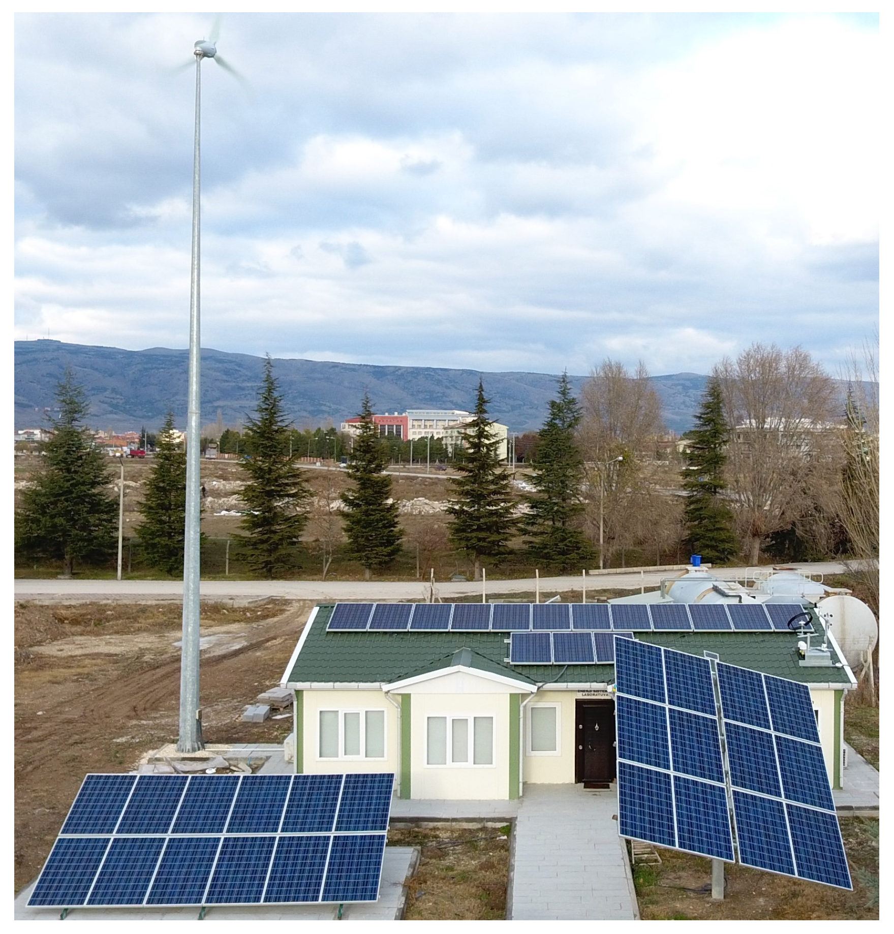
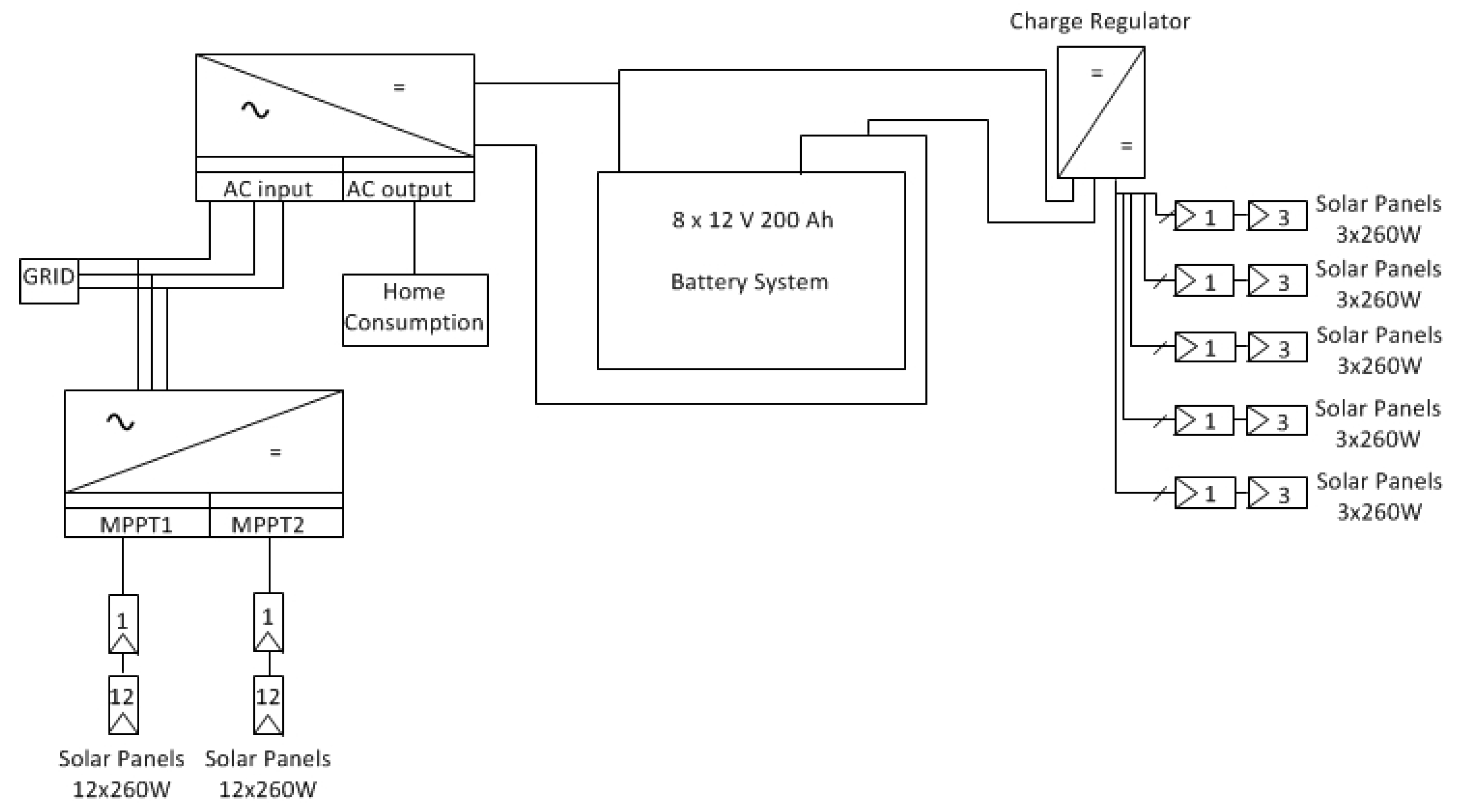
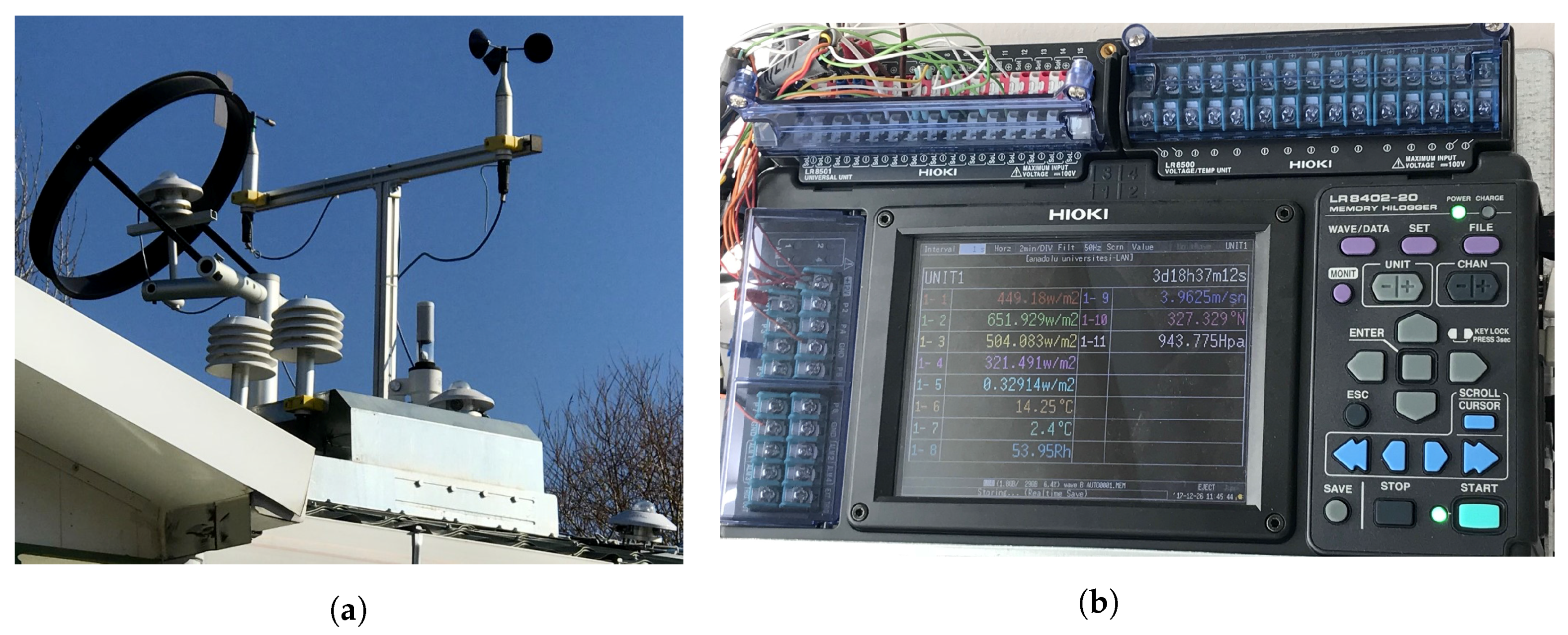
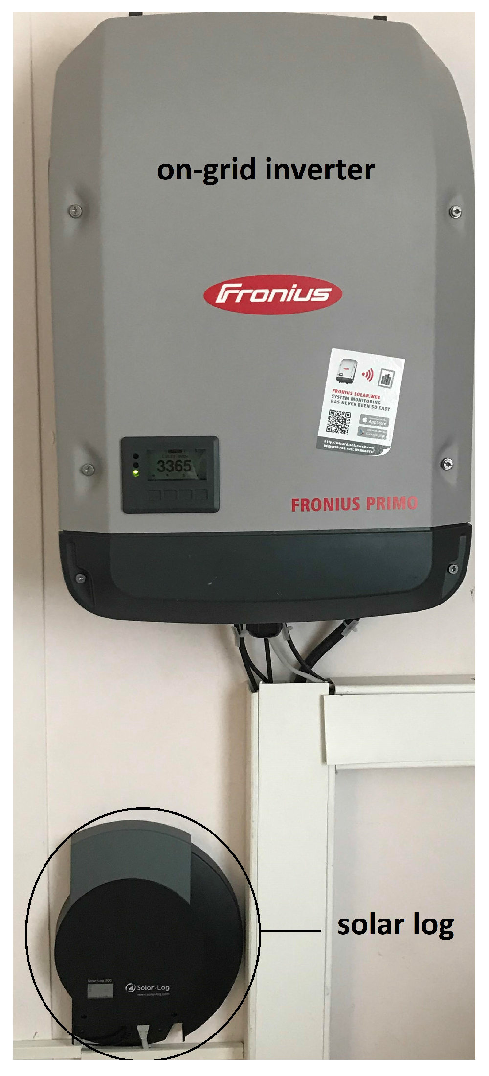
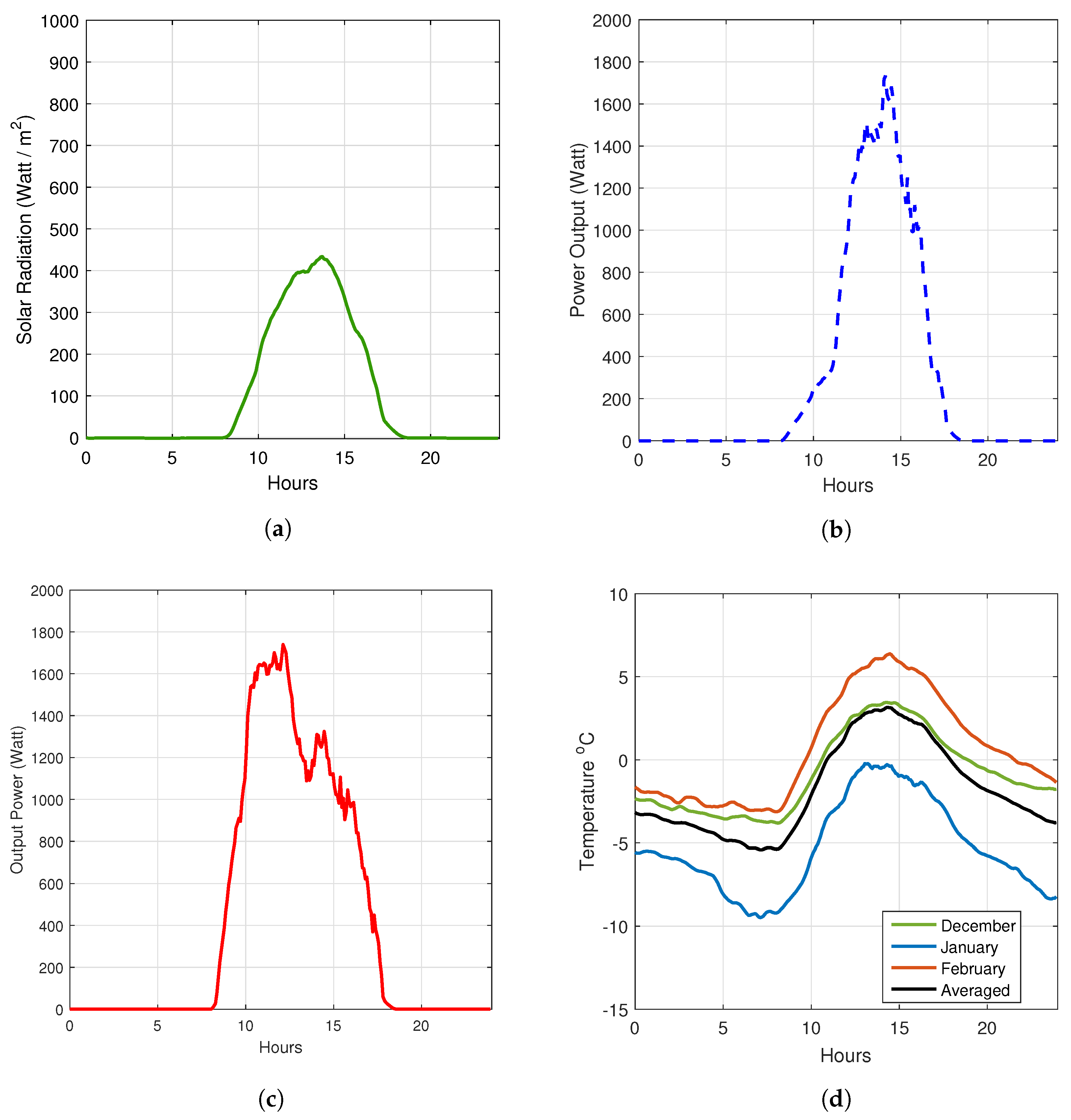
2. Description and Representation of the Solar System

The Renewable Energy Research Home (RERH) that was installed at Anadolu University İki Eylul Campus in Eskişehir, Turkey, consists of hybrid renewable energy generation units, various sensors, a data logger system, and an energy management system. Renewable energy generation and monitoring system consists of both on-grid and off-grid connected fixed and sun tracking solar PV panels on the roof and on the ground (a photograph is shown in Figure 1). The RERH is located in 39.78 latitude, 30.52 longitude at 794 m altitude.

The hybrid renewable generation system consists of 39 solar PV panels (3 kW ground fixed, 3 kW sun tracking and 4 kW roof-mounted) with 260 W for each panel and a 2.4 kW wind turbine with wireless two-way interface remote system. Roof-mounted solar panels are grid connected (on-grid) and the other fixed and sun tracking panels with equal capacity are off-grid (battery connected). The single axis sun tracking platform’s technical specifications can be summarized as; single axis, 90${}^{\circ }$ tracking angle along east-west, robust hot zinc-coated steel frame, ground installation on concrete foundation, stainless steel module fixings, maintenance-free DC linear drive, sensorless control, and self-powered with very low energy consumption. The electrical connections of all on/off inverters and batteries are designed as given in Figure 2.

A full weather measurement station with calibrated and precise sensors, and a real time data logging system is installed in the RERH. The weather measurement station includes a global radiation, direct radiation, diffuse radiation, sunshine duration, ambient temperature, cell temperature, ambient air humidity, wind speed, wind direction and weather pressure sensors as shown in Figure 3a. The acquired parameters are recorded in 1-s intervals using the data logging system depicted in Figure 3b. These high-rate recordings are then synchronized to the energy consumption intervals.

The technical specifications of the utilized pyranometer for solar radiation measurements are summarized in

Table 1. Technical specifications of the used pyranometer.

Specifications	Value
ISO 9060 classification	First Class
Response time 95% (s)	18
Sensitivity ($\mathsf{\mu }$V/Wm${}^{-2}$)	Approx. 7∼14
Impedance (Ω)	Approx. 20∼40
Operating temperature range (${}^{\circ }$C)	$-40$ to $+80$
Response time 95% (s)	data
Irradiance range (W/m${}^2$)	0–4000
Wavelength range	385 to 3000 nm

.

In the system, an on-grid inverter converts the variable direct current (DC) output of the PV solar panels into a utility frequency alternating current (AC) as shown in Figure 4. In the same figure, a solar log device also appears for observing and recording the total electricity generation values of both fixed and sun tracking PV panels separately as MPPT${}_1$ and MPPT${}_2$.

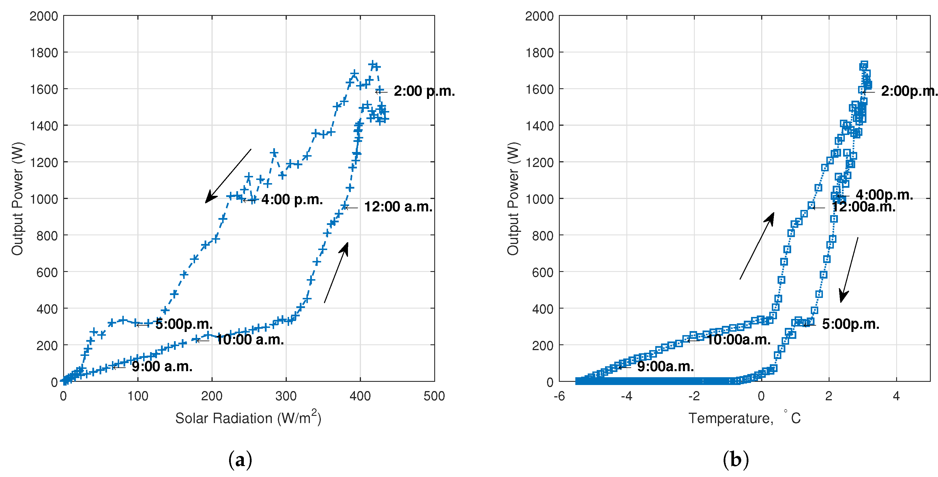
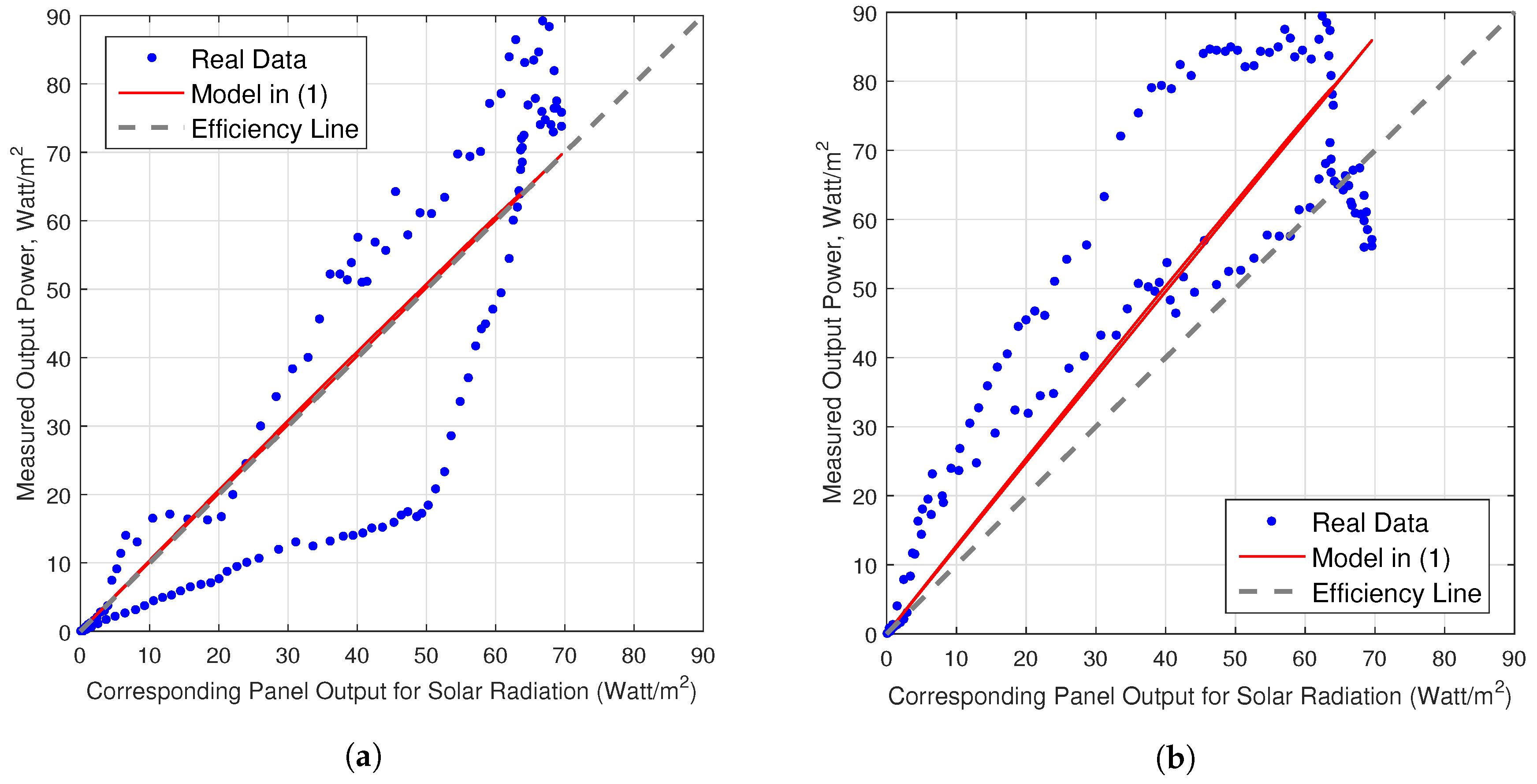
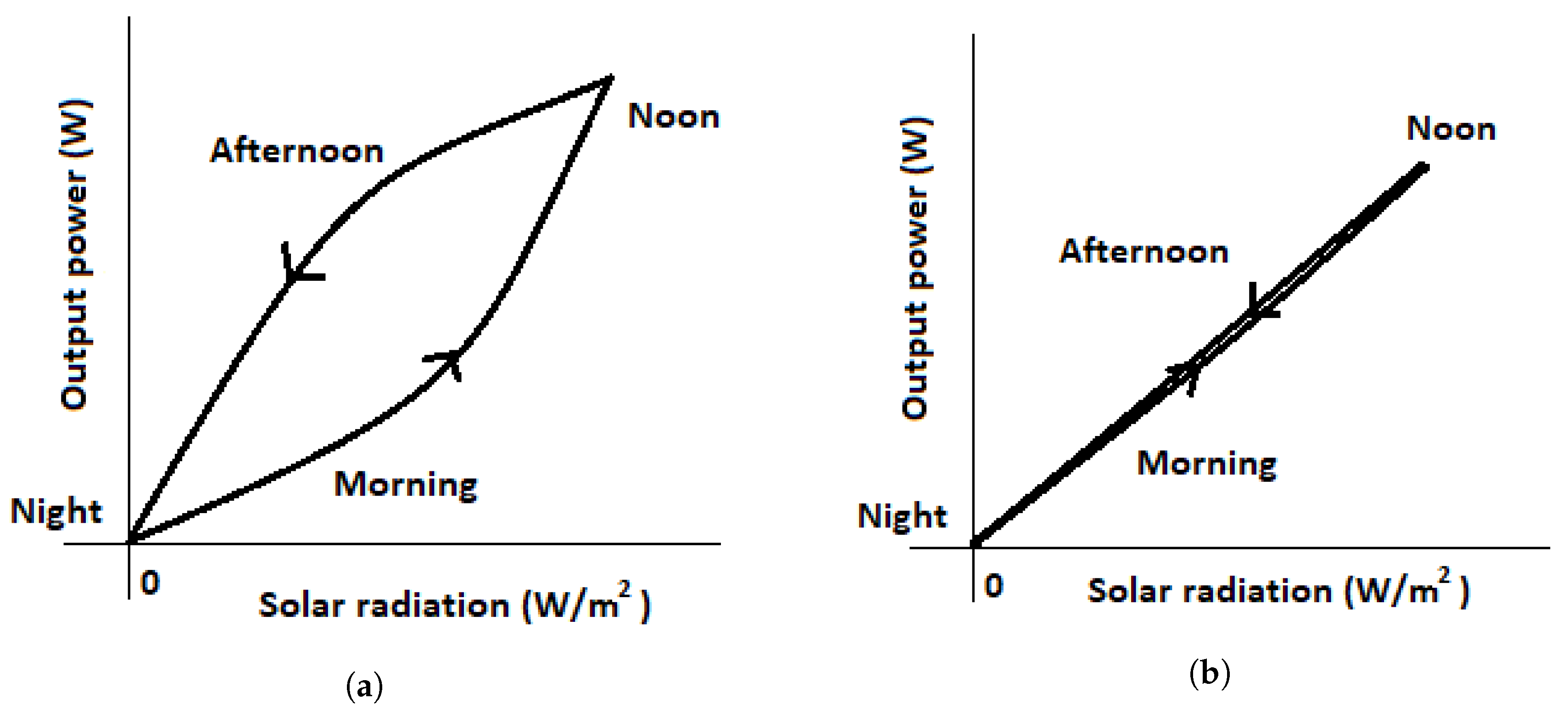
3. Solar PV Power Generation Models

In solar PV systems, the available global solar radiation (sun light) is converted into electricity using PV panels and inverters. The most commonly used (classical) model for estimating the conversion rate of solar radiation value into generated electricity power for maximum power point is empirically expressed in [3,19] as,

$$P\left(t\right)=\eta AG\left(t\right)(1-0.005(T\left(t\right)-25\left)\right)$$

(1)

where A is the total panel area (m${}^2$), $\eta$ is the system efficiency (%), $G\left(t\right)$ is the time-varying global solar radiation value (Watt/m${}^2$) and $T\left(t\right)$ is the ambient temperature value (${}^{\circ }$C) at time, t. There are some variations to this empirical model in the literature, including [5,7,10,14], yet this model is widely used in most applications, therefore this model is used as a benchmark for comparing our model results.

In order to test this model and construct an alternative one, our RERH system simultaneously recorded solar radiation values (W/m${}^2$), temperature (${}^{\circ }$C) and the corresponding actual output power throughout the days of the whole year. As a reference, averaged (for the winter days) global solar radiation values and fixed and sun-tracking PV panel output power values are shown in Figure 5a–c, respectively. It can be seen that, due to high variation of weather parameters (such as cloudiness, shading, etc.), the PV output values exhibit large fluctuations. Day-wise averaged ambient temperature values in winter are also given in Figure 5d.

In order to observe the time-varying relation of solar radiation (and of temperature) to the output power, these data are sequentially presented in Figure 6a,b. The interesting plot in Figure 6a indicates that, even at the same solar radiation levels, (say, 300 W/m${}^2$), different output powers are generated according to the time of the day. This may be clearly attributed to the warming-up of the panels; the morning hours at the same solar radiation level are usually colder as compared to the afternoon hours at the same solar radiation intensity. As a dual of this situation, from Figure 6b, it can be seen that even at the same temperature levels, different power output levels are observed this time due to the different solar radiations at the same temperatures. The common observation for both of these plots is the time-varying hysteresis behavior. In a previous work by the authors [34], this phenomenon was mentioned for the first time. In [34], the hysteresis behavior was attempted to be modeled using a 3-piece model (corresponding to morning, noon and afternoon). Since the hysteresis behavior of the temperature to output power relation was not noticed in that work, the temperature parameter was left out of the model. In this work, due to the observation in Figure 6b, the temperature values are added into the model and accurate conversion estimates are obtained.

The solar output values in Figure 6 show results of the 12 PV panels (each with 260 W capacity). During construction of the models, the values are scaled (or normalized) to eliminate effects of efficiency, losses and total panel area parameters. Hence, power values at the inverter output per m${}^2$ are obtained for the PV panels with recorded solar radiation and temperature point at maximum power point tracking (MPPT) mode. PV panels are open-air systems, therefore the lag of the output electrical energy production is attributed to the temperature dependency of the solar cells (yielding better efficiencies at the warmer temperatures of the afternoon). This model merely proposes a curve matching approach to the overall solar radiation-to-electric power phenomenon. The incapability of the classical model (which already incorporates the temperature in its conversion model) in Figure 8 implies that the presented lag may be caused by a more complicated heat dependence model or a different physical property, which requires deeper chemical and material analysis.

Figure 7 presents the differences between the actual and previous model’s conversion points at different times of the day (averaged for the winter season) for fixed and sun-tracking systems. The 45${}^{\circ }$ line is indicated as the efficiency line (which is the expected conversion according to the specifications of the panel), and the previous (classical) model output is rendered with a red line. The efficiency line for the sun-tracking system seems to underestimate the conversion. It can also be seen that the available classical model only marginally minimizes the model error (due to not considering the proposed lag effect). The time-wise blue dots render a deviation from the classical model (meaning a time-varying efficiency) lines, indicating a visible hysteresis effect.

The classical model that is shown as the red lines in Figure 7 corresponds to the normalized version of Equation (1), which can be re-written as:

$$P\left(t\right)=\eta G\left(t\right)(1+0.12T(t\left)\right),$$

(2)

where $P\left(t\right)$ is the model output of the power, $G\left(t\right)$ is the global solar radiation measured throughout winter days and $T\left(t\right)$ is the temperature. Here, $\eta$ is calculated separately for the fixed and sun-tracking systems to minimize the model error in the least square sense. It can be seen that the available classical model can only produce a daily average regression, and fails to track the instantaneous time variation of the actual output power values. Many of the available optimization efforts focus on better estimation of the efficiency line, while not considering the mentioned time-wise variations. The experimental data used herein can be accessed from the link in [38].

The proposed idea is a novel attempt to consider the instantaneous variations of the conversion curve. It is argued that the conversion figure exhibits a hysteresis behavior, which needs to be modeled separately for fixed and sun-tracking systems (as will be explained in the next section). The improvement in such a model is expected to have significance in applications which require instantaneous production estimations, such as bidding.

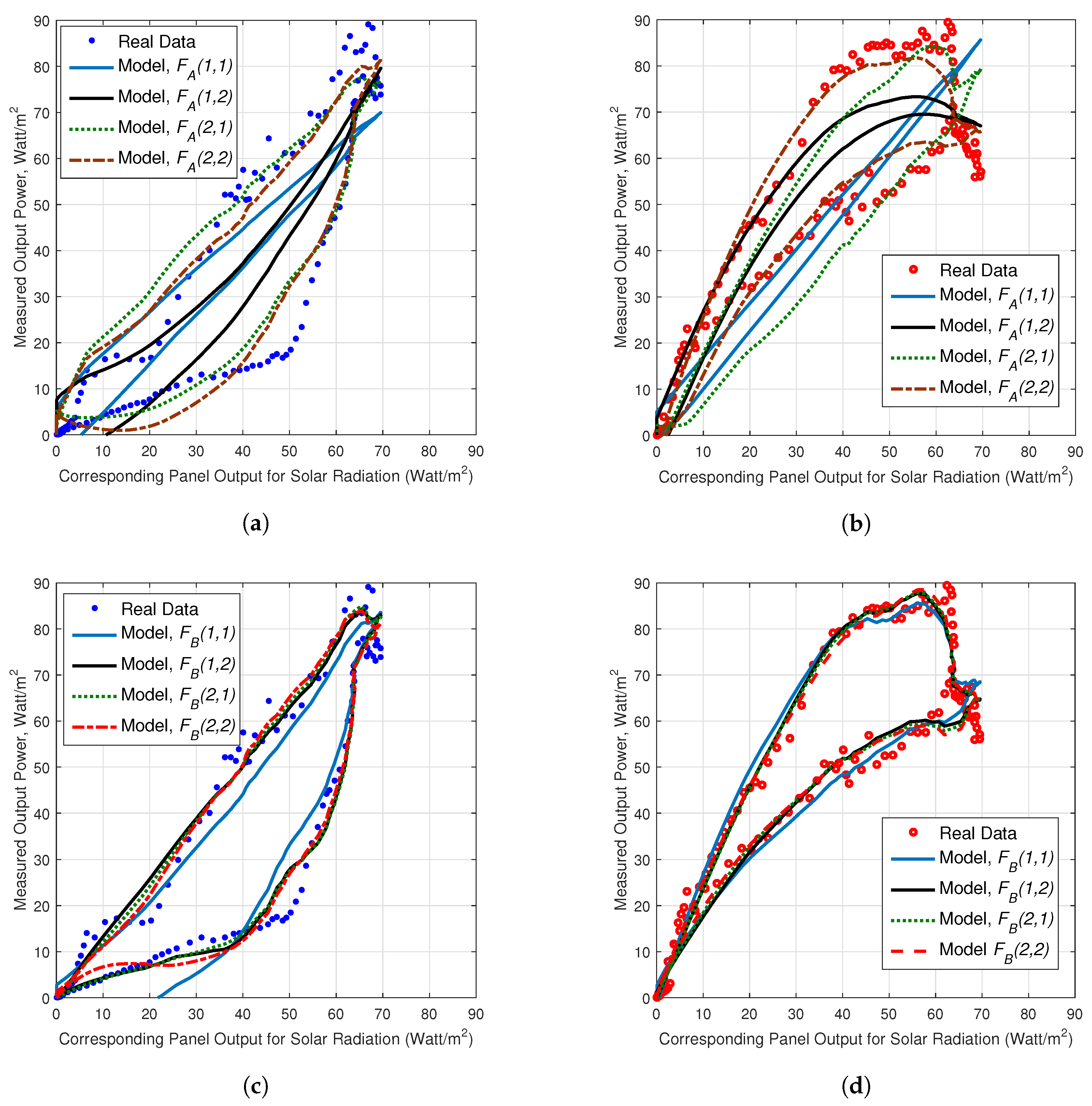
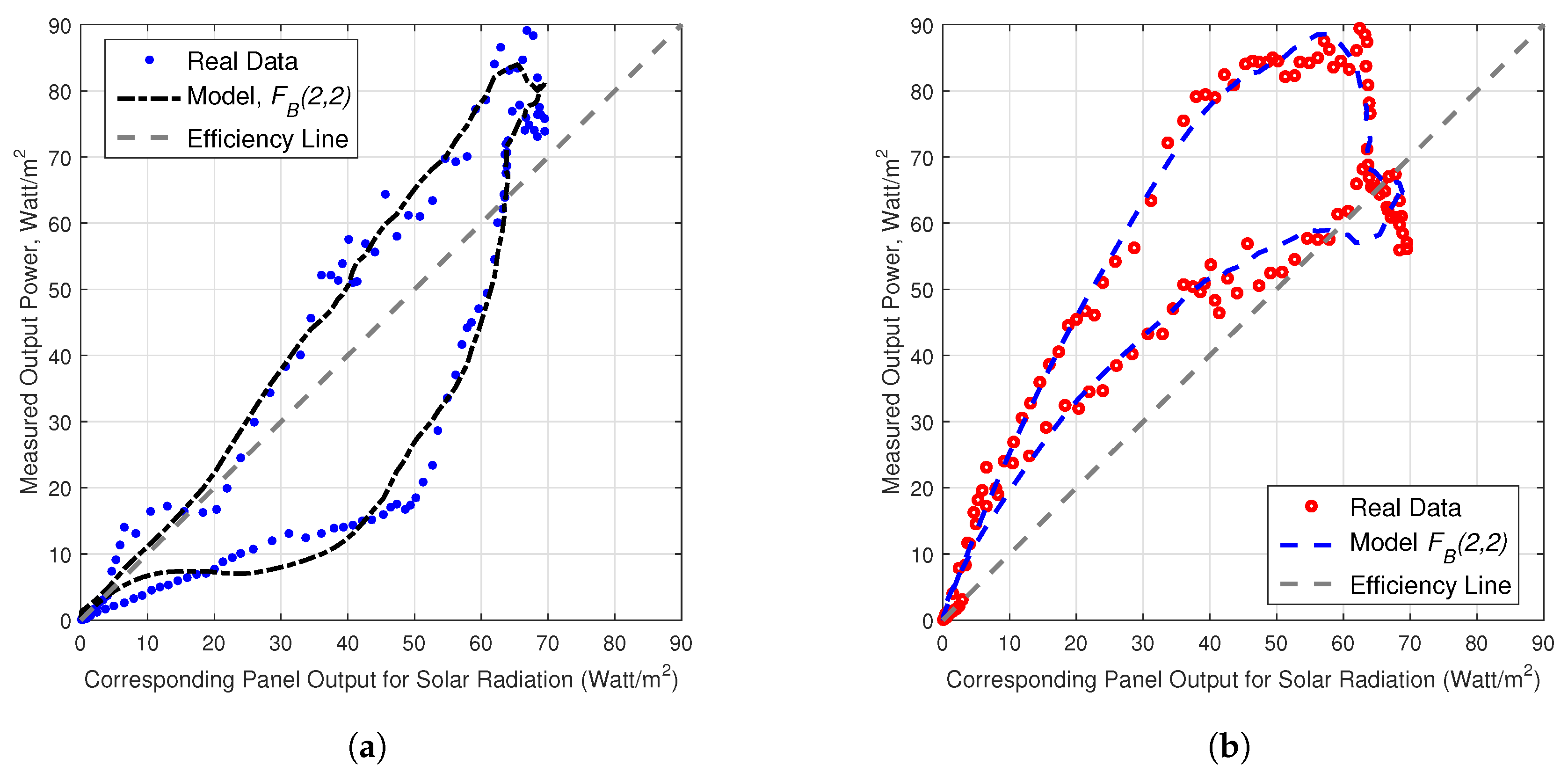
4. Hysteresis Models for PV Power Generation

As explained in the previous sections and as can be seen from Figure 6 and Figure 7, actual radiation-to-power conversion data needs an accurate model to handle time variations. In our previous study [34], it was observed that the global solar radiation-to-energy conversion phenomenon is not only non-linear, but it also has a strong time-varying characteristic. The hysteresis phenomenon is graphically illustrated in Figure 8a. The classical model is also illustrated in Figure 8b. The close-to-linear behavior of the classical model renders it difficult to depict the proposed hysteresis behavior.

In this section, novel models are proposed which are trained from real temperature, radiation and power data to depict the time-varying behavior using a single analytic expression. Two main approaches are proposed to achieve the best accuracy: additive and multiplicative:

$$F_A(p_1,p_2)=f_T\left(p_1\right)+f_G\left(p_2\right)$$

(3)

$$F_B(p_1,p_2)=f_T\left(p_1\right)\times f_G\left(p_2\right)$$

(4)

where $f_T\left(p_1\right)$ is the $p_1^{th}$ order polynomial temperature function such as

$$f_T\left(p_1\right)=a_1+a_{2}T\left(t\right)+\dots a_{p_1+1}{T}^{p_1}\left(t\right)$$

(5)

and $f_G\left(p_2\right)$ is the $p_2^{th}$ order polynomial global radiation function such as

$$f_G\left(p_2\right)=b_1+b_{2}G\left(t\right)+\dots b_{p_2+1}{T}^{p_2}\left(t\right).$$

(6)

In the polynomial expressions, ${\left\{a_i\right\}}_{i=1}^{p_1+1}$ and ${\left\{b_j\right\}}_{j=1}^{p_2+1}$ are real valued coefficients for the additive model. In order not to confuse with the multiplicative model parameters, a new set of polynomial coefficients of ${\left\{c_i\right\}}_{i=1}^{p_1+1}$ are used in the multiplicative model. High order polynomials are tested as models for the first time in the literature. In order to find the best fitting additive and multiplicative models with minimum order, eight different order levels are tested and presented in

Table 2. Proposed polynomial models for additive $F_A$ and multiplicative $F_B$ cases.

Model	Model Function
Model A-1	$F_A(1,1)=a_1+a_{2}T\left(t\right)+b_1+b_{2}G\left(t\right)$
Model A-2	$F_A(1,2)=a_1+a_{2}T\left(t\right)+b_1+b_{2}G\left(t\right)+b_3{G}^2\left(t\right)$
Model A-3	$F_A(2,1)=a_1+a_{2}T\left(t\right)+a_3{T}^2\left(t\right)+b_1+b_{2}G\left(t\right)$
Model A-4	$F_A(2,2)=a_1+a_{2}T\left(t\right)+a_3{T}^2\left(t\right)+b_1+b_{2}G\left(t\right)+b_3{G}^2\left(t\right)$
Model B-1	$F_B(1,1)=c_1+c_{2}T\left(t\right)+c_{3}G\left(t\right)+c_{4}T\left(t\right)G\left(t\right)$
Model B-2	$F_B(1,2)=c_1+c_{2}T\left(t\right)+c_{3}G\left(t\right)+c_4{G}^2\left(t\right)+c_{5}T\left(t\right)G\left(t\right)+c_{6}T\left(t\right)G^2\left(t\right)$
Model B-3	$F_B(2,1)=c_1+c_{2}T\left(t\right)+c_{3}G\left(t\right)+c_4{T}^2\left(t\right)+c_{5}T\left(t\right)G\left(t\right)+c_{6}G\left(t\right)T^2\left(t\right)$
Model B-4	$$\begin{gathered} F_B(2,2)=c_1+c_{2}T\left(t\right)+c_{3}G\left(t\right)+c_{4}T\left(t\right)G\left(t\right)+c_5{T}^2\left(t\right) \\ +c_6{G}^2\left(t\right)+c_7{T}^2\left(t\right)G\left(t\right)+c_{8}T\left(t\right)G^2\left(t\right)+c_9{T}^2\left(t\right)G^2\left(t\right) \end{gathered}$$

. It is, of course, possible to increase the order ($p_1$ and $p_2$) for the proposed models. However, in order to avoid overfitting, quadratic upper limits are proposed for $T\left(t\right)$ and $G\left(t\right)$.

The coefficients are optimized and the models are verified using data from east-west sun tracking and fixed solar PV panels throughout the winter season (the data is shared publicly in [38]). The coefficient optimization was performed in a least square sense. Detailed lists of model coefficients are given in

Table 3. Optimal coefficient values for model A both fixed and tracking PV system in Winter.

Winter			Fixed PV						Tracking PV
Model	$a_1$	$a_2$	$a_3$	$b_1$	$b_2$	$b_3$	$a_1$	$a_2$	$a_3$	$b_1$	$b_2$	$b_3$
$F_A(1,1)$	3.63	2.42	-	3.63	0.80	-	−0.92	−1.30	-	−0.92	1.31	-
$F_A(1,2)$	4.83	2.73	-	4.83	0.05	0.01	−3.23	−1.88	-	−3.23	2.74	−0.02
$F_A(2,1)$	3.66	8.03	1.42	3.66	0.47	-	−0.95	−6.53	−1.33	−0.95	1.62	-
$F_A(2,2)$	4.29	7.70	1.29	4.29	0.11	0.0064	−2.83	−5.57	−0.96	−2.83	2.70	−0.019

,

Table 4. Optimal coefficient values model B for fixed PV system.

Winter					Fixed PV
Model	$c_1$	$c_2$	$c_3$	$c_4$	$c_5$	$c_6$	$c_7$	$c_8$	$c_9$
$F_B(1,1)$	3.32	0.71	0.53	0.2	-	-	-	-	-
$F_B(1,2)$	−0.29	0.06	0.13	−0.026	0.082	0.0012	-	-	-
$F_B(2,1)$	0.24	0.055	1.03	−0.011	0.23	0.027	-	-	-
$F_B(2,2)$	2.08	1.22	0.46	0.27	0.16	−0.0006	0.08	−0.002	−0.0007

and

Table 5. Optimal coefficient values model B for sun tracking PV system.

Winter					Tracking PV
Model	$c_1$	$c_2$	$c_3$	$c_4$	$c_5$	$c_6$	$c_7$	$c_8$	$c_9$
$F_B(1,1)$	3.14	0.86	1.65	−0.25	-	-	-	-	-
$F_B(1,2)$	1.43	0.34	1.72	0	−0.13	−0.002	-	-	-
$F_B(2,1)$	0.97	0.22	1.97	−0.005	−0.18	−0.019	-	-	-
$F_B(2,2)$	2.37	1.55	1.82	−0.25	0.22	−0.0025	−0.012	0.0011	−0.0003

. The values of the corresponding coefficients that were optimized according to the minimum root mean square error (RMSE) and mean absolute error (MAE) are presented in

Table 6. MAE and RMSE values for fixed and tracking PV panel output power values (Watt) in Winter.

Winter	Fixed PV		Tracking PV
Model	MAE	RMSE	MAE	RMSE
$F_A(1,1)$	4.3185	8.1754	5.2961	9.5833
$F_A(1,2)$	3.7231	7.1004	3.2360	5.8737
$F_A(2,1)$	2.0609	4.0130	3.5432	6.4949
$F_A(2,2)$	2.0721	3.7568	1.9204	3.7438
$F_B(1,1)$	2.2234	4.1080	1.5329	3.0344
$F_B(1,2)$	1.2839	2.5657	1.3383	2.7015
$F_B(2,1)$	1.2709	2.5111	1.3249	2.6481
$F_B(2,2)$	1.2833	2.3537	1.2928	2.5578
[2,3,19,20]	4.8780	4.8780	5.4692	10.07

. The utilized definitions of RMSE and MAE are given in Equations (7) and (8):

$$\mathrm{RMSE}=\sqrt{\frac{1}{N}\sum _{t=1}^{t=N}{(P\left(t\right)-F_{A,B}\left(t\right))}^2}$$

(7)

$$\mathrm{MAE}=\frac{1}{N}\sum _{t=1}^{t=N}|P\left(t\right)-F_{A,B}\left(t\right)|$$

(8)

where $P\left(t\right)$ is the measured real panel output power and $F_{A,B}\left(t\right)$ is proposed model power output value with N being the total averaged data points. All of the optimized models are plotted together with the real input data in Figure 9.

According to the error values in Table 6 and Figure 9, an immediate observation is that the multiplicative model $F_B(2,2)$ yields the best results, while all the proposed methods already outperform the available classical model in terms of accuracy (which was shown as the last column with a label of [2,3,19,20]). Therefore, this model ($F_B(2,2)$) is separately plotted for fixed and sun tracking cases in model Figure 10a,b. In both of the figures, it can be seen that the model curves successfully track actual data.

Considering that all of the presented methods (including the classical model) require a data collection period for parameter optimization, it is claimed that the proposed models have a clear advantage in minimizing the model error by successfully revealing the time-varying hysteresis behavior. Another advantage of the proposed model is that, unlike the previous hysteresis attempt in [34], these polynomial functions (i) are single analytical (not piecewise) and (ii) consider temperature information for greater accuracy.

As a conclusion of these numerical studies, it is argued that the proposed models significantly improve the accuracy of power output conversion value, which is critical in applications that require optimum bidding strategy [2].

5. Conclusions

Due to the importance of optimal bidding in current and future smart grid applications, accurate estimation of instantaneous power from available solar panels remains to be an important and active problem. This study presents a novel approach for solar radiation-to-power output conversion by observing a time-varying behavior of real life conversion data from the RERH system on our campus. The classical state-of-the-art model only considers a linear relation between ambient temperature/solar radiation and output power, disabling the possibility of incorporating the eminent hysteresis behavior which causes a time variation in the conversion. In this work, various models are proposed to enable the system to incorporate a time varying relation of the solar radiation-to-power conversion. The proposed models naturally provide a superset of the classical models. It can be noticed that, for instance, if we set $c_1$ and $c_2$ in Model B-1 to zero, $c_3=\eta$ and $c_4$ to $0.12\times \eta$, we obtain the classical model. Therefore, the conversion modeling accuracy of the proposed models are always expected to perform at least as good as (and, in most cases, better than) the classical model. In order to emphasize the advantage of the proposed model, the winter season is chosen as the data observation period, which shows greater variations in weather conditions. The RERH system was active with several sensors that record the data at high sampling rates (mostly 1 sample/s). Similarly, the output power production was also monitored, therefore real conversion values were obtained. When the conversion values are plotted on the solar radiation vs. output power axis, the hysteresis curve became clear. By using polynomial models to depict the effect of solar radiation and temperature in a time-varying manner, eight model candidates were obtained. Interestingly, each of these models individually outperform the classical model, both in fixed and sun-tracking PV cases, with the multiplicative model ($F_B(2,2)$) achieving the best accuracy. As in the case of the other state-of-the-art methods, the proposed model parameters need to be trained according to the data acquired from the installation plant. Since the test of the system accuracy is performed on a central location inside Anatolia, geographically similar locations (around the same latitudes, such as many places in Europe, Middle East-to-Japan and USA) are expected to yield similar solar radiation-to-power conversion values, enabling the proposed methods to outperform the classical conversion models. It remains an interesting problem to verify these models at different geographical locations (i.e., tropic rain forests, deserts or arctic regions), yet the ability of revealing a rich class of conversion curves (including the hysteresis curves) renders the proposed method a strong and plausible alternative to existing conversion models.

References

1. Filik, T.; Basaran Filik, Ü. Efficiency Analysis of the solar tracking PV systems in Eskisehir. Anadolu Univ. J. Sci. Technol. A 2017, 18, 209–217. [Google Scholar] [CrossRef]
2. Nguyen, D.T.; Le, L.B. Optimal bidding strategy for microgrids considering renewable energy and building thermal dynamics. IEEE Trans. Smart Grid 2014, 5, 1608–1620. [Google Scholar] [CrossRef]
3. Chen, S.X.; Gooi, H.B.; Wang, M. Sizing of energy storage for microgrids. IEEE Trans. Smart Grid 2012, 3, 142–151. [Google Scholar] [CrossRef]
4. Ulbricht, R.; Fisher, F.; Lehner, W.; Donker, H. First Steps Towards a Systematical Optimized Strategy for Solar Energy Supply Forecasting. In Proceedings of the European Conference on Machine Learning and Principles and Practice of Knowledge Discovery in Databases, Prague, Czech Republic, 23–27 September 2013. [Google Scholar]
5. Dolara, A.; Leva, S.; Manzolini, G. Comparison of different physical models for PV power output prediction. Sol. Energy 2015, 119, 83–99. [Google Scholar] [CrossRef] [Green Version]
6. Fernandez-Jimenez, L.A.; Muñoz-Jimenez, A.; Falces, A.; Mendoza-Villena, M.; Garcia-Garrido, E.; Lara-Santillan, P.; Zorzano-Alba, E.; Zorzano-Santamaria, P.J. Short-term power forecasting system for photovoltaic plants. Renew. Energy 2012, 44, 311–317. [Google Scholar] [CrossRef]
7. Dunea, A.; Dunea, D.; Moise, V.; Olariu, M. Forecasting methods used for performance’s simulation and optimization of photovoltaic grids. In Proceedings of the 2001 IEEE Porto Power Tech Proceedings, Porto, Portugal, 10–13 September 2001. [Google Scholar]
8. Monteiro, C.; Santos, T.; Fernandez-Jimenez, L.A.; Ramirez-Rosado, I.J.; Terreros-Olarte, M.S. Short-term power forecasting model for photovoltaic plants based on historical similarity. Energies 2013, 6, 2624–2643. [Google Scholar] [CrossRef]
9. Martín, L.; Zarzalejo, L.F.; Polo, J.; Navarro, A.; Marchante, R.; Cony, M. Prediction of global solar irradiance based on time series analysis: Application to solar thermal power plants energy production planning. Sol. Energy 2010, 84, 1772–1781. [Google Scholar] [CrossRef]
10. Ogliari, E.; Grimaccia, F.; Leva, S.; Mussetta, M. Hybrid predictive models for accurate forecasting in PV systems. Energies 2013, 6, 1929–2013. [Google Scholar] [CrossRef] [Green Version]
11. Ji, W.; Chee, K.C. Prediction of hourly solar radiation using a novel hybrid model of ARMA and TDNN. Sol. Energy 2011, 85, 808–817. [Google Scholar] [CrossRef]
12. Dolara, A.; Grimaccia, F.; Leva, S.; Mussetta, M.; Ogliari, E. A Physical hybrid artificial neural network for short term forecasting of PV plant power output. Energies 2015, 8, 1138–1153. [Google Scholar] [CrossRef] [Green Version]
13. Hocaoglu, F.; Gerek, O.N.; Kurban, M. Hourly solar radiation forecasting using optimal coefficient 2-D linear filters and feed-forward neural networks. Sol. Energy 2008, 8, 714–726. [Google Scholar] [CrossRef]
14. Mellit, A.; Massi, P.A. A 24-h forecast of solar irradiance using artificial neural network: Application for performance prediction of a grid-connected PV plant at Trieste, Italy. Sol. Energy 2010, 84, 807–821. [Google Scholar] [CrossRef]
15. Simonov, M.; Mussetta, M.; Grimaccia, F.; Leva, S.; Zich, R.E. Artificial intelligence forecast of PV plant production for integration in smart energy systems. Int. Rev. Electr. Eng. 2012, 7, 3454–3460. [Google Scholar]
16. Zhu, H.; Li, X.; Sun, Q.; Nie, L.; Yao, J.; Zhao, G. A power prediction method for photovoltaic power plant based on wavelet decomposition and artificial neural networks. Energies 2015, 9, 9–11. [Google Scholar] [CrossRef]
17. Izgi, E.; Oztopal, A.; Yerli, B.; Kaymak, M.K.; Şahin, A.D. Short-mid-term solar power prediction by using artificial neural networks. Sol. Energy 2012, 86, 725–733. [Google Scholar] [CrossRef]
18. Zeng, J.; Qiao, W. Short-term solar power prediction using a support vector machine. Renew. Energy 2012, 52, 118–127. [Google Scholar] [CrossRef]
19. Tao, C.; Shanxu, D.; Changsong, C. Forecasting Power Output for Grid-Connected Photovoltaic Power System without using Solar Radiation Measurement. In Proceedings of the 2010 2nd IEEE International Symposium on Power Electronics for Distributed Generation Systems (PEDG), Hefei, China, 16–18 June 2010; pp. 773–777. [Google Scholar]
20. Yona, A.; Senjyu, T.; Funabashi, T. Application of Recurrent Neural Network to Short-Term-Ahead Generating Power Forecasting for Photovoltaic System. In Proceedings of the 2007 IEEE Power Engineering Society General Meeting, Tampa, FL, USA, 24–28 June 2007; pp. 1–6. [Google Scholar]
21. Tijjani, B.I. Comparison between first and second order Angstrom type models for sunshine hours at Katisna, Nigeria. Bayero J. Pure Appl. Sci. 2011, 4, 24–27. [Google Scholar]
22. El-Metwally, M. Sunshine and global solar radiation estimation at different sites in Egypt. J. Atmos. Sol. Terr. Phys. 2005, 67, 1331–1342. [Google Scholar] [CrossRef]
23. Khalil, S. A; Fathy, A.M. An empirical method for estimating global solar radiation over Egypt. Acta Polyechnica 2008, 48, 48–53. [Google Scholar]
24. Elagib, N.; Mansell, M.G. New approaches for estimating global solar radiation across Sudan. Energy Convers. Manag. 2000, 21, 271–287. [Google Scholar] [CrossRef]
25. Sarsah, E.A.; Uba, F.A. Monthly-specific daily global solar radiation estimates based on sunshine hours in Wa, Ghana. Int. J. Sci. Technol. Res. 2013, 2, 246–254. [Google Scholar]
26. Gairaa, K.; Bakelli, Y. A comparative study of some regression models to estimate the global solar radiation on the horizontal surface from sunshine duration and meteorological parameters for Ghardaia site, Algeria. ISRN Renew. Energy 2013, 2013, 754956. [Google Scholar] [CrossRef]
27. Falayi, E.O.; Adepitan, J.O.; Rabiu, A.B. Empirical models for the correlation of global solar radiation with meteorological data for Iseyin, Nigeria. Int. J. Phys. Sci. 2008, 3, 210–216. [Google Scholar]
28. Okonkwo, G.N.; Nwokoye, A.O.C. Estimating global solar radiation from temperature data in Minna location. Eur. Sci. J. 2014, 10, 1857–7431. [Google Scholar]
29. Adeala, A.A.; Huan, Z.; Enweremadu, C.C. Evaluation of global solar radiation using multiple weather parameters as predictors for South Africa Provinces. Therm. Sci. 2015, 19, 495–509. [Google Scholar] [CrossRef]
30. Kolebaje, O.T.; Sika, A.I.; Akinyemi, P. Estimating solar radiation in Ikeja and Port Harcourt via correlation with relative humidity and temperature. Int. J. Energy Prod. Manag. 2016, 1, 253–262. [Google Scholar] [CrossRef]
31. Ayvazogluyuksel, O.; Basaran Filik, U. Estimation of monthly average hourly global solar radiation from the daily value in Canakkale, Turkey. J. Clean Energy Technol. 2017, 5, 389–393. [Google Scholar] [CrossRef]
32. Deepak, V.; Nema, S.; Shandilya, A.M.; Soubhagya, K.D. Maximum power point tracking (MPPT) techniques: Recapitulation in solar photovoltaic systems. Renew. Sustain. Energy Rev. 2016, 54, 1018–1034. [Google Scholar]
33. Sharma, N.; Sharma, P.; Irwin, D.; Shenoy, P. Predicting Solar Generation from Weather Forecasts Using Machine Learning. In Proceedings of the 2011 IEEE International Conference on Smart Grid Communications (SmartGridComm), Brussels, Belgium, 17–20 October 2011. [Google Scholar]
34. Filik, T.; Basaran Filik, Ü.; Gerek, Ö.N. Solar radiation-to-power generation models for one-axis tracking PV system with on-site measurements from Eskisehir, Turkey. In Proceedings of the E3S Web of Conferences, Wałbrzych, Poland, 21–22 September 2017. [Google Scholar]
35. Mayergoyz, I. Mathematical Models of Hysteresis and their Applications; Elsevier Series; Electromagnetism Academic Press: New York, NY, USA, 2003; ISBN 9780124808737. [Google Scholar]
36. Snaith, H.J.; Abate, A.; Ball, J.M.; Eperon, G.E.; Leijtens, T.; Noel, N.K.; Stranks, S.D.; Wang, J.T.; Wojciechowski, K.; Zhang, W. Anomalous hysteresis in perovskite solar cells. J. Phys. Chem. Lett. 2014, 5, 1511–1515. [Google Scholar] [CrossRef] [PubMed]
37. Unger, E.L.; Hoke, E.T.; Bailie, C.D.; Nguyen, W.H.; Bowring, A.R.; Heumüller, T.; Christoforo, M.G.; McGehee, M.D. Hysteresis and transient behavior in current-voltage measurements of hybrid-perovskite absorber solar cells. Energy Environ. Sci. 2014, 7, 3690–3698. [Google Scholar] [CrossRef]
38. Basaran Filik, Ü.; Filik, T.; Gerek, Ö.N. Global Solar Radiation, Temperature, Sun-Tracking and Ground Fixed Solar PV Power Generation Data Set for Winter Season from RERH. Available online: https://data.mendeley.com/datasets/vxg4t8yn6j/1 (accessed on 31 January 2018).
Figure 1. The Renewable Energy Research Home (RERH) at Anadolu University İki Eylul Campus in Eskişehir, Turkey.
Energies 11 00603 g001
Figure 2. The electrical connections of all on/off grid inverters and batteries.
Energies 11 00603 g002
Figure 3. (a) Sensors of the weather measurement station; (b) Screen view of multichannel real time data logging device.
Energies 11 00603 g003
Figure 4. On-grid inverter with solar log.
Energies 11 00603 g004
Figure 5. (a) Averaged global solar radiation values in winter; (b) Averaged fixed photovoltaic (PV) panel power output values in winter; (c) Averaged output power values of sun tracking PV panels in winter; (d) Averaged ambient temperature values.
Energies 11 00603 g005
Figure 6. (a) Solar radiation to output power; (b) Temperature to output power.
Energies 11 00603 g006
Figure 7. Measured output power value and corresponding panel output for solar radiation model in (1): (a) Fixed system; (b) Sun-tracking system.
Energies 11 00603 g007
Figure 8. (a) Hysteresis curve; (b) Current, state of the art (classical) model.
Energies 11 00603 g008
Figure 9. Actual and model output power values: (a) Model A for fixed system; (b) Model A for tracking system; (c) Model B for fixed system; (d) Model B for tracking system.
Energies 11 00603 g009
Figure 10. Measured output power value and corresponding panel output for solar radiation for proposed model in F B ( 2 , 2 ) : (a) Fixed system; (b) Tracking system.
Energies 11 00603 g010