Abstract
Power balance, including active and reactive power, between the system supply and the demand from induction motor loads is a potentially necessary condition for system stable operation. Motion of system states depends on the balancing of active and reactive powers. Therefore, this paper proposes an induction machine model in electromechanical timescale from a power balancing viewpoint, in which the induction motor load is modeled as a voltage vector driven by power balancing between the system supply and the demand from induction motor load, so as to describe the dynamic characteristics of induction motor loads in a physical way for power system dynamic analysis. Then a voltage magnitude-phase dynamic analysis with the proposed induction machine model is constructed. Based on the voltage magnitude-phase dynamic analysis, the characteristics of grid-connected induction motor loads are explored, and the instability mechanisms of grid-connected induction motor loads induced by a large disturbance are discussed. It is shown that the dynamic behavior of grid-connected induction motor loads can be described as the dynamic process of the terminal voltage vector driven by coupled active and reactive power balancing in different timescales. In this way, the dynamic behavior of induction motor loads in terms of voltage magnitude-phase dynamics and its physical characteristics are clearly illustrated. Time-domain simulation results are presented to validate the above analyses.
1. Introduction
Induction machines are an important element in power systems. Approximately 60% to 70% of the total energy supplied by a power system is consumed by induction motor (IM) loads such as industrial and commercial motor loads and household air conditioners [1]. Recent researches on induction motors mainly include induction machine drive, design of novel machine, fault diagnosis [2,3,4,5], etc., while study of power systems dynamic with directly connected IM loads reduces. In fact, the IM loads are the main reactive power load in power systems and play a key role in system operation of different kinds of power systems, including utility grid, microgrid, and so on. For the operation of utility grid, blackout accident will cause serious economic damages [6,7], while the characteristics of IM is one of the important factors in such issue studies. Thus, it is understandable that the voltage collapses experienced by the Western Systems Coordinating Council (WSCC) system on both 10 August 1996 and 4 August 2000 cannot be properly reproduced by simulations that do not contain dynamic IM loads [8,9]. In addition to the utility grid, IMs also impact the operation of microgrids. As for microgrids equipped with energy management system, the distinctive autonomous operational capability of microgrids improves the reliability of electricity companies in supplying power demands when microgrids operate at autonomous mode [10,11]. However, microgrids can be subjected to a high penetration level of induction motor loads, and the highly nonlinear IM loads dynamics may challenge the stability of microgrids [12]. Besides, although the newly installed wind turbines are connected to grid through power electronics and researches are mainly focus on novel control strategy of these machines [13,14], a certain number of Type 1 induction generators are still operating in conventional wind farms [15]. As a result, the dynamic behavior of induction machines has a significant impact on power system stability.
Representation of IM loads in power systems has been investigated in many studies. Mathematical equation descriptions of equivalent IM circuits have been developed with various levels of detail, including a detailed 5th order model, a reduced 3rd order model, and a much reduced 1st order model [16]. These IM models are widely used in small-signal stability studies [17,18], where the IM is represented as a transient voltage on the d-q axis [17] or as a small-signal admittance [18], in steady state analysis [19] and in transient performance research of grid-connected IM loads [20,21] and grid-connected Types 1 induction generators [15,22]. However, the mathematical description of induction machines makes it difficult to comprehend the dynamic characteristics of IMs from a physical perspective because of the multi-variable, nonlinear and strongly coupled nature of the equations. Although the eigenvalue analysis method, the time domain simulation method and the multi-variable frequency domain analysis [23] are both applicable to IM model analysis, the complex coupled relationship among electrical quantities is concealed. When it comes to a large complex system, it becomes even more difficult to comprehend the physical mechanisms behind the phenomena and explore further insights into system dynamic characteristics.
Practical operational problems have also promoted the development of IM load models for large-scale interconnected system operations studies. Motivated by an accident in the Swedish blackout of 1983, some IM load models based on measurements and simulation have been proposed, where active power is a function of the time derivation of the voltage magnitude [24], or where reactive power is related to the time derivation of the voltage magnitude [25]. Such an apparent discrepancy is caused by overlooking the coupled active and reactive power features in the induction machines. Besides, the algebraic and differential equations, in which active or reactive power is a function of voltage magnitude, are used to represent the induction machine for analyzing static flow and voltage stability [26], while the effect of system frequency is usually disregarded. However, IM loads are very sensitive to system frequency variation [16,27], and power systems can experience large frequency excursions during a severe system fault.
Power balance between the system supply and the demand from IM loads that includes both active and reactive power is a potentially necessary condition for stable operation. Note that, the sufficiency requirement for stable operation includes not only the power balance but also the property of a power system that enables it to remain in a state of operating equilibrium under normal operating condition and to regain an acceptable state of equilibrium after being subjected to a disturbance [28]. The balancing of active and reactive powers is a key mechanism of power system dynamic stability driving the evolution of system states. Therefore, describing the dynamic behavior of devices states from the perspective of power balancing can help to clearly illustrate the physical relationship between those devices states. Although active power balancing between the demand and the supply has been previously proposed for voltage stability in [29], the coupled active and reactive power features in power systems, and the voltage phase that reflects the effects of frequency, were neglected. Consequently, it is of vital importance to establish an induction machine model that contains voltage magnitude-phase dynamics and electric power features to properly demonstrate the physical characteristics underlying dynamic response.
In this vein, this paper proposes an induction machine model in electromechanical timescale from the power balancing viewpoint, in which both the terminal voltage magnitude and phase in the IM loads are considered as being driven by power balancing between the system supply and the demand from IM loads. In addition, further work is conducted by applying the proposed IM model to characteristic study and stability analysis. More specifically, the concepts of multi-timescale coupling and coupled power balancing are explored for describing dynamic behavior of grid-connected IM loads, and the instability mechanisms of grid-connected IM loads are discussed. From active and reactive power balancing viewpoint, the dynamic performance of the IMs is summarized in terms of voltage magnitude-phase dynamics, which helps to illustrate the dynamic behavior of IM loads and its physical characteristics for power systems dynamic analysis. Besides, the evolution of the voltage magnitude is clarified by the power balancing, which provides a new perspective for voltage stability analysis.
The rest of this paper is structured as follows. Section 2 introduces the concept of power balancing and presents the proposed IM model, with a verification also provided. In Section 3, a voltage magnitude-phase dynamic analysis is conducted, in which the concepts of multi-timescale coupling and coupled power balancing are explored for describing the dynamic behavior of grid-connected IM loads. Section 4 elaborates on the physical mechanisms of instability from the concept of power balancing, and relevant simulation studies are carried out to validate the analyses. Section 5 discusses original modeling intentions and future applications of the proposed IM model, while Section 6 summarizes this work.
2. Proposed Induction Machine Model
This section models an IM from the perspective of power balancing, which consists of: (1) reactive power balancing between the IM demand and network supply; (2) active power balancing between the IM demand and network supply; and (3) the balancing between air-gap power and mechanical power in the IM. Based on this proposed IM model, we then present a verification using a time-domain simulation.
2.1. Concept of Power Balancing in Grid-Connected IM Loads
The studied system is shown in Figure 1a in which the induction motor loads are connected to generations through AC transmission lines and transformers. In order to focus on the study of IMs characteristic, the IM-connected grid is simplified into an infinite bus in the following text, shown in Figure 1b. In the electromechanical timescale, the fast dynamics of both the transient process of the stator and rotor reactance can be ignored. Thus, the IM features can be described by steady state equivalent circuit shown in Figure 1c and rotor motion.
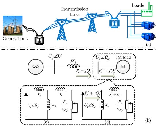
Figure 1.
The studied system: (a) the physical diagram of the studied system; (b) simplified single- induction motor (IM) infinite-bus system; (c) IM steady state equivalent circuit; (d) simplified IM steady state equivalent circuit.
(1) Reactive power balancing between the IM demand and network supply
Given an infinite bus and lumped the transmission and sub-transmission lines reactance and transformer reactance into xg, the power Pe + jQe supplied by the network in Figure 1b is
where Ug is the infinite bus voltage, and Ut and θut are the terminal voltage magnitude and phase.
Since xm is usually considerably larger than xs, the IM steady state equivalent circuit shown in Figure 1c can be simplified to the system shown in Figure 1d. Thus the power Pe* + jQe* demanded by the IM can be described by
where xs and xr are the stator and rotor leakage reactance, xm and Rr are the magnetizing reactance and rotor resistance, sslip is the slip.
Eliminating θut from (1) and (2) gives
Similarly, eliminating sslip from (3) and (4) obtains
In (6), the minus sign corresponds to the low slip (high-speed) operating point, while the plus sign corresponds to the high slip (low-speed) operating point.
It can be seen from (5) and (6) that the characteristics of the reactive power with respect to the terminal voltage magnitude Ut on the supply side are completely different from the demand side when transmitting a given active power. Note that Qe represents the reactive power features of the network supply while Qe* represents the reactive power features of the IM demand. Although (5) and (6) present different reactive power features, the terminal voltage magnitude Ut will be fixed when there is a reactive power balance between the IM demand and network supply.
Figure 2 plots Qe and Qe* with respect to terminal voltage magnitude. As can be seen from the figure, the intersection points of the two kinds of reactive power curves are the operating points, and the right points (namely points A and B) are the stable operating points. That is, in the neighborhood of the stable operating point, the terminal voltage magnitude decreases when Qe* > Qe and increases when Qe* < Qe. In other words, when the IM-required reactive power is larger than the supplied reactive power, the unbalanced reactive power drives a decrease in terminal voltage magnitude. Conversely, if the IM-required reactive power is smaller than the supplied reactive power, the unbalanced reactive power will increase the terminal voltage magnitude. Therefore, we can determine the dynamic behavior of the terminal voltage magnitude subjected to the unbalanced reactive power.
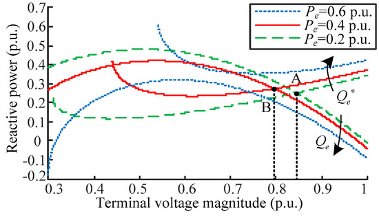
Figure 2.
Q-U static characteristics of a single-IM infinite-bus system.
Note that the capacitor that usually compensates for the IM is not included in Figure 1. Thus, the terminal voltage magnitude of the IM operates below the normal level. In case of a capacitor support, the network supplied power is affected and improved, while the characteristic of the power demanded by the IM does not change. Therefore, with the help of the capacitor, the terminal voltage magnitude can be raised to rated voltage in weak grid.
We can also see from Figure 2 that the stable operating point moves left and the terminal voltage magnitude decreases with increasing transmitted active power. When the transmitted active power is 0.6 p.u., there are no intersection points between Qe and Qe*. Furthermore, Qe* > Qe always holds at any terminal voltage magnitude, which means the voltage will decrease until the motor stalls. This indicates that the system has a maximum transmitted active power due to the reactive power balance constraint.
(2) Balancing of active power between the IM demand and network supply
Eliminating θut from (1) and (2) can also provide the active power Pe supplied by the infinite bus. Similarly, eliminating sslip from (3) and (4) gives the active power Pe* of the IM demand. Therefore, when transmitting a given reactive power, an active power balancing exists between IM demand and network supply. From (5) and (6), it is clear that the active power balancing is coupled with the reactive power balancing. Note, however, that a similar derivation is not repeated in this section.
(3) Balancing of mechanical power and air-gap power in an IM
The rotor motion in an IM reflects the balancing between mechanical power and air-gap power according to
where Pe* represents the air-gap power that is the numeric equivalent of the IM-demanded active power [29], H is the inertia, ωr is the rotor speed, and Pm* is the mechanical power that can be modeled as a quadratic mechanical power characteristic
The relationship between slip, slip frequency, and rotor speed can be written as
where ωs is the stator frequency, and
and θut is the terminal voltage phase.
Using the equations developed in this section, an IM model including three sets of power balancing can now be proposed.
2.2. Proposed IM Model Based on Power Balancing
It is important to make sure the procedures are clear before modeling. Figure 3 shows the block diagram of power balancing based method for IMs modeling. In Figure 3, the modeling of IM can be divided into two parts. The left part of Figure 3 relates to the balancing of mechanical power and air-gap power, and the right part of Figure 3 relates to the electric active and reactive power balancing. These power balancing are coupled with each other driving the motion of IM outputs. By combing Figure 3 with specific equations of IM presented in (3), (4) and (7)–(10), a power-balancing based induction machine model is illustrated as a block diagram in Figure 4, where the supplied powers Qe and Pe are the inputs, and Ut and θut are the outputs.
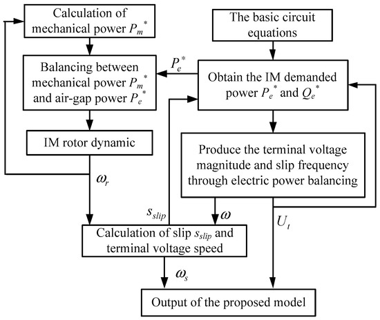
Figure 3.
The block diagram of proposed method for IM modeling.
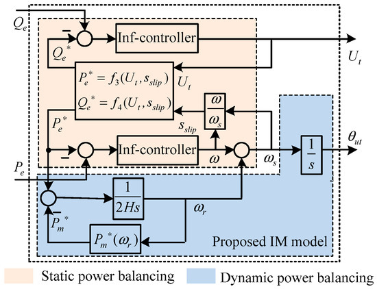
Figure 4.
Proposed induction machine model.
In Figure 4, the power balancing is performed by analogizing the feedback control, in which the power demanded by the IM is the reference and the network supplied power is the feedback. When there is unbalanced electric power between IM demand and network supply, an “inf-controller” will instantly regulate the terminal voltage magnitude Ut and slip frequency ω. If there is also an imbalance between mechanical power and air-gap power, the rotating frequency of terminal voltage vector ωs will vary with both slip frequency ω and rotor speed ωr, thus increasing or decreasing the terminal voltage phase θut. The inf-controller is responsible for the instantaneous regulation of the operating point from one state to another in the condition of electric power balancing (for example, moving from point A to B in Figure 2 when Pe changes from 0.2 p.u. to 0.4 p.u.). Note that the inf-controller presented here is more to identify the relation between the unbalanced electric power and state. However, the inf-controller can be realized in simulation by algorithm, the details for which will be explained in the following part.
2.3. Model Verification
The proposed induction machine model was verified by comparing results from the model to those from the detailed model in MATLAB/Simulink. The system shown in Figure 1b was implemented. The transmission line and IM rotor inertia here alone are 0.1 p.u. and 3 s, respectively. The remaining parameters are listed in the Appendix A. Based on the explanation in Section 2.2, the inf-controller can be implemented as a dogleg trust-region algorithm [30]. We assume that a −0.2 p.u. disturbance in infinite voltage occurs at 4 s.
Figure 5a–d show the comparative responses of input active and reactive power, terminal voltage phase relative to infinite voltage phase −θut, and terminal voltage magnitude Ut between the proposed and detailed models with Pm* = 0.2 p.u. respectively. By comparing the simulation results with the proposed model and detailed model, the observed difference can be attributed to the electromagnetic transients neglected in simulation with proposed IM model. Note that the proposed IM model is mainly used for power system dynamic analysis in electromechanical timescale. Based on this proposed induction machine model, a detailed dynamic performance of grid-connected IM loads will be discussed in following section.
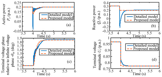
Figure 5.
Comparison of simulation responses between the proposed and detailed models when the magnitude of Ug decreases 0.2 p.u. at 4 s: (a) active power; (b) reactive power; (c) terminal voltage phase relative to infinite voltage phase; (d) terminal voltage magnitude.
3. Dynamic Performance of Grid-Connected IM loads in terms of Voltage Magnitude-Phase Dynamics
The dynamic behavior of IM loads in power systems is usually overlooked. However, such behavior has a significant influence on power system stability. This section explains the dynamic performance of grid-connected IM loads using the proposed IM model. The concepts of multi-timescale coupling and coupled power balancing are introduced first. Then a voltage magnitude-phase dynamic analysis is conducted in a single-machine system.
The section of the block diagram in Figure 4 highlighted in yellow is referred to as the static power balancing for the instantaneous response of the power balancing. Correspondingly, the area highlighted in blue in the diagram is referred to as the dynamic power balancing for the rotor inertia. Obviously, the static power balancing responds faster than the dynamic power balancing. Therefore, the dynamic behavior of IM loads is the coupled result of different timescale responses, i.e., multi-timescale coupling. This behavior can be analyzed for disturbances over different timescales, such as short timescale disturbances and long timescale disturbances. When considering short timescale disturbances, the dynamic power balancing can be ignored due to its slow response. In the short timescale, the dynamic is instantaneous following a disturbance and only the static power balancing responds. For long timescale disturbances, the dynamic power balancing affects the static power balancing through the rotor speed. In the long timescale, the rotor motion in IMs acts typically over several seconds following a disturbance. In this case, the dynamic behavior of the IM loads contains both dynamic and static power balancing.
In addition to the multi-timescale coupling, there is also the coupled power balancing in induction machines. Figure 6 shows the block diagram of a system dynamic analysis for a single-IM infinite-bus system, where the dotted lines are plotted for discussing the effects of coupled power balancing. It can be seen from the figure that the terminal voltage magnitude Ut is closely related to the reactive power balancing. However, the blue dotted line in Figure 6 shows that the terminal voltage magnitude Ut also affects both the active power supply Pe and the active power demand Pe* through the external transmission network and the IM load (i.e., f3--f4(Ut, sslip)), respectively. Similarly, as the yellow dotted line in Figure 6 illustrates, the frequency and phase are not only closely related to the active power balancing but also affect the reactive power balancing. Therefore, balancing of the active and the reactive power is mutually coupled through the IM load and the external transmission network.
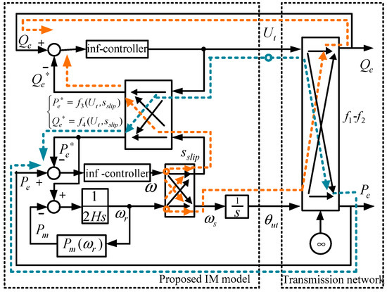
Figure 6.
System dynamic analysis block diagram for a single-IM infinite-bus system.
With the concepts of multi-timescale coupling and coupled power balancing introduced, we next discuss in detail the dynamic performance of grid-connected IM loads under short and long timescale disturbances from the aspect of voltage magnitude-phase dynamics.
3.1. Dynamic Performance of Grid-Connected IM Loads under a Short Timescale Disturbance
Using Figure 6, the following describes the detailed dynamic process of grid-connected IM loads after a short timescale disturbance. Note that the rotor speed is assumed invariable in this case as there is insufficient time for rotor speed to respond.
Network transmitted electric power affected by the disturbance: A 0.2 p.u. step down disturbance in the magnitude of the infinite voltage occurs at 2 s. From (1) and (2), it is quite clear that the network transmitted electric power Pe + jQe will instantly decrease. The time-domain simulation results are depicted in Figure 7a,b. The solid line in Figure 7a shows the active power response under a short timescale disturbance, and the solid line in Figure 7b is the reactive power response under a short timescale disturbance.
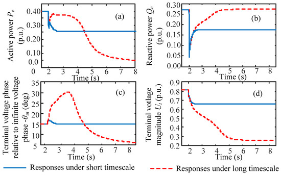
Figure 7.
Dynamic response of IM loads under short timescale (solid) and long timescale (dashed) disturbances: (a) active power; (b) reactive power; (c) terminal voltage phase relative to the infinite voltage phase; (d) terminal voltage magnitude.
Terminal voltage vector responds to the power supplied from the network: From the left part of Figure 6, the balancing of Pe and Pe* and the balancing of Qe and Qe* are affected when the reduced electric power Pe + jQe transfers to the IM. The results of imbalanced electric power lead to the change of terminal voltage vector. The detailed processes of the terminal voltage change are explained as follows. This change can be analyzed from the proposed induction machine model. We first assume the IM-demanded power Pe* + jQe* is invariable, and that the unbalanced power between IM demand and network supply will drive the terminal voltage magnitude Ut and slip frequency ω. Finally, the changed terminal voltage magnitude Ut and slip frequency ω regulate the IM-demanded power Pe* + jQe* through f3--f4(Ut, sslip) to balance the static power. The above process leads to a decrease in terminal voltage magnitude Ut, and the slip frequency ω holds constant. Moreover, the terminal voltage rotating vector ωs is invariable according to (9), thus leading the terminal voltage phase relative to the infinite voltage phase −θut invariable. The simulation results are shown in Figure 7c,d, with constant −θut before and after disturbance. The solid line in Figure 7c is the response of terminal voltage phase relative to infinite voltage phase, and the solid line in Figure 7d is the terminal voltage magnitude response. Note that the time-domain simulation results under short timescale in Figure 7 are plotted using the detailed model, thus the results contain the electromagnetic dynamic which is ignored in analysis.
Network transmitted electric power affected by the terminal voltage vector: Note that the varying terminal voltage vector will in turn change the transmitted power, as shown in the right part of Figure 6. According to (1) and (2), the decline in terminal voltage magnitude Ut decreases the transmitted active power Pe and increases the reactive power Qe. The results are shown in Figure 7, with both the active and reactive power decreasing. Note that, the active power finally cannot return to the previous value since the rotor motion is ignored under the short timescale dynamic.
Closed loop forms: The electric power changed in the steps above will in turn affect the terminal voltage vector. Eventually, the above steps develop into a closed loop, and repeat until the system finds an equilibrium point.
3.2. Dynamic Performance of Grid-Connected IM Loads under a Long Timescale Disturbance
When the IM is subjected to a long timescale disturbance, the rotor motion remains a factor and must be considered. The motor mechanical power is modeled as a quadratic to the rotor speed (shown in (8)). Here we still assume a −0.2 p.u. disturbance occurring in the infinite voltage magnitude at 2 s. As shown in Figure 7a,b, the disturbance still causes the electric active and reactive power to step down instantly. In Figure 7a, the dashed line represents the response of active power. The dashed line in Figure 7b is the response of reactive power.
The changed electric power transferred to the IM affects the terminal voltage vector. In this case, the process that terminal voltage vector responds to the power supplied from the network, which, as shown in part A, needs to consider not only the static power balancing but also the dynamic power balancing.
Static power balancing in the IM: Regulation of the terminal voltage vector for static power balancing is similar to what occurred in the short timescale disturbance shown in part A. The terminal voltage magnitude Ut eventually decreases.
Dynamic power balancing in the IM: Since the static power balancing is faster than dynamic power balancing, the results from the static power balancing will affect the dynamic power balancing. That is, the system state (i.e., the terminal voltage magnitude Ut) driven by static power balancing will affect dynamic power balancing through the air-gap power Pe*. Therefore, it is obvious that Pe* (i.e., the IM demand active power) decreases due to the decreased terminal voltage magnitude Ut, and the reduced air-gap power interacting with the mechanical power further affects the rotor speed. Figure 8a shows the reduced air-gap power after the disturbance. The unbalanced power between air-gap power and mechanical power decelerates the rotor speed.
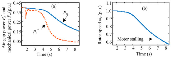
Figure 8.
Dynamic response of IM loads (a) mechanical power Pm and air-gap power Pe*; (b) rotor speed ωr.
The result of static and dynamic power balancing in the IM is that the terminal voltage rotating vector slows down according to (9) due to the decelerated rotor speed ωr. As a result, −θut increases.
The changing terminal voltage vector will in turn affect the transmitted electric power and eventually form a closed loop. The detailed dynamic process is similar to the process described in part A. In Figure 8a, the dynamic process causes the air-gap power to remain less than the mechanical power. Therefore, ωr will keep decreasing until the rotor stalls, shown in Figure 8b. The mechanism for the system experiencing instability, i.e., the instability mechanism, will be illustrated in Section 4.
To summarize the dynamic performance of a grid-connected induction machine in parts A and B: (1) under a short timescale disturbance, the dynamic process of the terminal voltage vector is driven by the coupled static active power balancing and reactive power balancing; and (2) under a long timescale disturbance, the dynamic process of the terminal voltage vector is driven by the coupled static and dynamic power balancing.
4. Instability Mechanism of Grid-Connected IM Loads from a Power Balancing Viewpoint
From the dynamic analysis in Section 3, we know that the IM states, which can reflect the system stability, are driven by the power balancing. This section will now illustrate the instability mechanism of grid-connected IM loads from the power balancing viewpoint. Note, however, that the processes for regulating rotor speed and terminal voltage phase are ignored. Since the IM characteristics are separated from the transmission network by power balancing in this work, rather than being lumped together as they have been in other studies [31], it is possible to conduct an in-depth investigation into the instability mechanisms.
Two types of grid-connected IM load operating conditions after a disturbance, namely, abnormally low voltage and stalling, will be discussed in this section. In a practical power system, there is typically low voltage load shedding protection installed on IM loads to disconnect the motor if the voltage falls below a given threshold. However, in order to analyze the mechanism behind this instability phenomenon, such low voltage load shedding protection will not be considered in this work. Similarly, protection that can avoid IM stalling is also not included in the following analysis.
4.1. Abnormally Low Voltage Analysis
Operation at a low voltage indicates that, although the voltage of the operating point is considerably below the allowed level, IM static power balancing and dynamic power balancing are still in equilibrium. This can occur due to the quadratic nature of the mechanical power.
Consider the system shown in Figure 1b. Since the static power between the IM demand and network supply is balanced before and after the disturbance, the air-gap power Pe* obtained from the terminal voltage can be derived from the infinite voltage by
In (11), the air-gap power Pe* is a function of infinite voltage Ug and slip sslip. The stator frequency ωs is maintained at 1.0 p.u. since we neglect the terminal voltage phase regulation. Hence, the relationship between rotor speed ωr and slip sslip, as shown in (9), can be transformed to
Similarly, the mechanical power Pm* shown in (8) can be transformed to the function of slip sslip
Figure 9a illustrates the mechanical power and air-gap power with respect to slip according to (11) and (13). As shown in the figure, there are three intersection points when the infinite voltage is 1.0 p.u., and only the middle operating point is unstable. When the infinite voltage Ug is 0.8 p.u., the only intersection point, i.e., the only stable operating point, is close to a standstill for the rotor. The change in infinite voltage corresponds to a step down disturbance of the infinite voltage magnitude. The practical operating point is A before the disturbance, and point B after the disturbance.
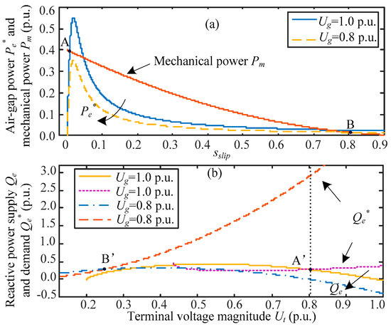
Figure 9.
Abnormally low voltage analysis: (a) air-gap power Pe* and mechanical power Pm versus slip curves; (b) reactive power supply Qe and reactive power demand Qe* versus terminal voltage magnitude Ut curves.
Figure 9b shows the reactive power Qe and Qe* versus terminal voltage magnitude Ut at 1.0 p.u. and 0.8 p.u. infinite voltage, respectively, corresponding to the reactive power balancing using (5) and (6). The intersection points of Qe and Qe* at 1.0 p.u. and 0.8 p.u. infinite voltage are marked as points A’ and B’, which correspond to points A and B in Figure 9a.
The characteristics of the reactive power versus voltage of the IM loads for Qe* in Figure 9b represent completely different characteristics under different infinite voltages. With a drop in infinite voltage, a massive reactive power is required to continue operating near the previous voltage (i.e., point A’). Therefore, we can see from Figure 9b that the reactive power Qe* corresponding to point A’ is considerably larger than Qe after the disturbance. That is to say, the reactive power demand is far more than the reactive power supplied by the power system, causing the terminal voltage to decrease until both reactive powers are equal. Ultimately, Figure 9a,b illustrate that the system eventually reaches an abnormally low voltage to maintain a power balance, namely points B and B’.
Time-domain simulation results are shown as a three-dimensional diagram in Figure 10, where the magnitude of the infinite voltage steps down from 1.0 p.u. to 0.8 p.u. at 2 s. The blue lines in Figure 10a are the mechanical power, the green lines are the air-gap power, and the red line is the practical operating point. The blue lines in Figure 10b are the reactive power supply, the green lines are the reactive power demand, and the red line is the practical operating point. As illustrated by the figure, the system operates at stable points A and A’ before the disturbance. After the disturbance, both the active power versus slip and reactive power versus voltage change over time, and finally terminal voltage magnitude reaches an abnormally low voltage that corresponds to the post-disturbance equilibrium points B and B’. This time domain simulation verifies the theoretical analysis from the previous section.
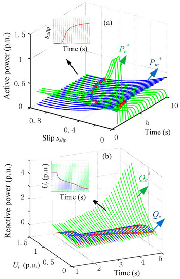
Figure 10.
Three-dimensional diagram of an abnormally low voltage after a disturbance: (a) air-gap power and mechanical power versus slip curves; and (b) reactive power demand and supply versus terminal voltage magnitude curves.
4.2. IM Stalling Analysis from a Power Balancing Viewpoint
The process in which the rotor speed of an IM decelerates to a complete stop is referred to as stalling. According to the dynamic performance of an IM, stalling signifies that the electric power and mechanical power are unbalanced. Since the quadratic mechanical power always intersects the electrical power at a stable operating point, we can assume a constant mechanical power of 0.4 p.u. in this case. Similar to the work described in [29], the mechanisms causing IM stalling for the system shown in Figure 1 have been summarized as ST1 and ST2. However, here we will illustrate these mechanisms from a reactive power balancing standpoint, and in terms of the balancing between air-gap power and mechanical power.
Similar to ST1 and ST2, IM stalling can be summarized as: (1) no operating points of intersection between the reactive power demand and supply, and no balance between the mechanical power and air-gap power; and (2) a lack of attraction for the operating points towards a stable post-fault reactive power equilibrium.
(1) No operating points of intersection between the reactive power demand and supply, and no balance between the mechanical power and air-gap power
According to (5) and (6), Figure 11a is reactive power demand Qe* and supply Qe versus Ut at 1.0 p.u. and 0.8 p.u. infinite voltage. There are two intersection points, A’ and B’, for a 1.0 p.u. infinite voltage. When the IM is subjected to a −0.2 p.u. disturbance in infinite voltage, Qe decreases. Since Qe* is independent of the infinite voltage because of (4), Qe* is invariable before and after the disturbance. In this case, there is no intersection point between Qe and Qe* after the disturbance. As a result, the IM stalls.
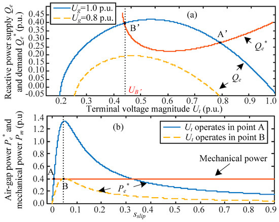
Figure 11.
IM stalling analysis: (a) reactive power supply Qe and reactive power demand Qe* versus terminal voltage magnitude Ut curves; (b) air-gap power Pe* and mechanical power Pm versus slip curves.
This result is confirmed by the power balancing between air-gap power Pe* and mechanical power Pm. Pe* is a function of the terminal voltage magnitude and slip according to (3). Pe* under different terminal voltage magnitudes is plotted in Figure 11b, and corresponds to the terminal voltage magnitude of points A’ and B’ in Figure 11a. It can be seen from Figure 11a that, after the disturbance, Qe* is larger than Qe. Thus, the terminal voltage magnitude starts to decrease, which also corresponds to the decline in Pe* seen in Figure 11b. When the terminal voltage magnitude decreases to point B’ in Figure 11a, Pe* and Pm in Figure 11b are exactly tangent to one another. If the terminal voltage magnitude keeps decreasing, there will be no intersection points between Pe* and Pm. At this stage, the IM stalls. Since there are no intersection points between Qe and Qe* after the disturbance, there are also no intersection points between Pe* and Pm.
(2) A lack of attraction for the operating points towards a stable post-fault reactive power equilibrium
Using Figure 11a, suppose the system initially operates at point A’. The system is then subjected to a −0.2 p.u. disturbance in the infinite voltage. This fault makes Qe decline. Since Qe* is larger than Qe, the terminal voltage magnitude starts to decrease. If the fault is cleared when the terminal voltage magnitude is larger than that of point B’ (namely UB’ shown in Figure 11a), then the post-fault Qe will be larger than Qe*. In this case, the net reactive power will increase the terminal voltage magnitude until it reaches the pre-fault operating point. If the fault is cleared when the terminal voltage magnitude is smaller than UB’, then the post-fault Qe will be smaller than Qe*. In this case, the net reactive power will decrease the terminal voltage magnitude until the IM stalls.
Time-domain simulation results are shown in Figure 12, where a −0.2 p.u. step down disturbance is imposed on the infinite voltage magnitude. The system first operates at point A (A’). After the disturbance, ωr and Ut drops. If the fault is not cleared, the IM stalls. If the fault is cleared at UB’, the rotor speed and the terminal voltage magnitude return to their initial values. If, on the other hand, the fault is cleared below UB’, the rotor speed decelerates to a stall. These simulation results agree very well with the analytical results described above.
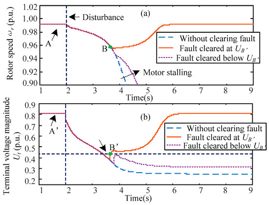
Figure 12.
Time-domain simulation of IM stalling after a disturbance: (a) rotor speed; and (b) terminal voltage magnitude.
5. Discussion
The characteristics of grid-connected devices, namely their response when subject to a disturbance, is one of the key factors influencing the dynamic behavior of power systems. Since the devices of diversified characteristics perplex the system dynamic behavior as well as the mechanisms behind these phenomena, it is necessary to find a general way to represent the characteristics of different devices for power system dynamic analysis. Generally, voltage magnitude and phase are the two major aspects of system dynamic stability, and the balancing of active and reactive powers is a key mechanism of power system dynamic stability driving the evolution of system states. Therefore, we can represent a grid-connected device using a voltage magnitude-phase state driven by the device’s active and reactive power balancing. As active power, reactive power, and voltage magnitude-phase state exist in every device, the characteristics of a variety of grid-connected devices, such as VSCs, SGs, and induction machines, can generally be described and modeled from this perspective. Take the wind turbine model as an example, differ to the wind turbine models for power system stability analysis in time-domain [32,33,34], this modeling method can intuitively reflect the physical relation between the power balancing and states. In this way, the essential difference in characteristics among different devices can be recognized.
Combined with the IM loads, this paper proposed a voltage magnitude-phase model driven by coupled active and reactive power balancing. This power-balancing based model can apply to multi-machine dynamic analysis exploring the physical mechanism. As Figure 13 shows the variation of the phase and magnitude in one device will lead to the changes in the power and voltage vector of all other devices through the power network. Correspondingly, the total power in the IM load is the sum of the power component from the IM load itself resulting from the voltage phase and magnitude, plus the power components from other devices as well. The dynamics of the IM load in a multi-machine system is thus affected by the power balancing between the power demand in the IM and the power supply from the other devices. The detailed analysis depends on the properties of the devices and the network structure. In addition, the proposed IM model is applicable to system frequency response study and voltage stability analysis. For example, an IM’s available inertia can be deduced and used for analyzing frequency stability using the proposed IM model. Since reactive power balancing drives the dynamic evolution of the voltage magnitude in the proposed IM model, the voltage stability problem can be explored by consulting the angle stability. Owing to the complexity of these problems, the above topic will be analyzed in future work.
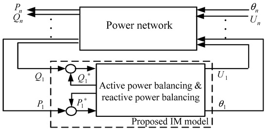
Figure 13.
Schematic diagram of a multi-machine system containing the proposed model.
6. Conclusions
This paper proposed an induction machine model that intuitively describes the dynamic behavior of an IM load and its physical characteristics for power system dynamic analysis. The induction machine was first modeled as a terminal voltage vector driven by power balancing between the system supply and the demand from IM loads. Using the proposed IM model, a voltage magnitude-phase dynamic analysis was then developed to explore the dynamic characteristics of grid-connected IM loads. Based on the voltage magnitude-phase dynamic analysis, the characteristics of multi-timescale coupling and coupled power balancing in the IMs were introduced and used to analyze the dynamic performance of grid-connected IM loads. The analysis showed that the dynamic performance of grid-connected IM loads can be described in the following manner: (1) under short timescale disturbances, the dynamic process of the terminal voltage vector is driven by coupled static active and reactive power balancing; (2) under long timescale disturbances, the dynamic process of the terminal voltage vector is driven by coupled static and dynamic power balancing. This summary contributes to clarify the IMs’ characteristics of coupled active and reactive power versus voltage magnitude-phase in different timescales and can help to promote understanding the dynamic characteristics of IMs in complex large systems. Furthermore, two types of unstable operating conditions in grid-connected IM loads, namely abnormally low voltage and stalling, were analyzed using the conclusion of the dynamic performance. The instability mechanisms, particularly the evolution of the voltage magnitude, were well explained by reactive power balancing between the IM demand and the network supply, as well as balancing of air-gap power and mechanical power. Simulation results supported these analyses. Investigation of multi-machine systems containing IM loads using the proposed model will be presented in future works.
Acknowledgments
The work presented in this paper was fully supported by the grant from the National Key Research and Development Program of China (2016YFB0900104) and the grant from the Basic Research Project of Qinghai Province of China (2016-ZJ-767). The authors would like to thank Pro. Jiabing Hu from SEEE, Huazhong University of Science and Technology, for his help on the paper.
Author Contributions
Ding Wang, Xiaoming Yuan and Meiqing Zhang propose the main idea of the paper. Ding Wang implements the mathematical derivations, simulation verifications and analyses. The paper is written by Ding Wang and is revised by Xiaoming Yuan and Meiqing Zhang.
Conflicts of Interest
The authors declare no conflict of interest.
Nomenclature
| Ug, xg | Infinite bus voltage, transmission line reactance |
| Pe, Qe | Active and reactive power transmitted from the network |
| Ut, θut | Terminal voltage magnitude and phase |
| Pe*, Qe* | Active power (air-gap power) and reactive power of induction motor demand |
| xs, xr | Stator and rotor leakage reactance |
| xm, Rr | Magnetizing reactance, rotor resistance |
| H, sslip | Induction motor inertia and slip |
| ωs, ωr, ω | Stator frequency, rotor speed, slip frequency |
Appendix A
Infinite bus: Ug = 400 V, fbase = 50 Hz.
The grid equivalent reactance (including the reactance of transmission line and transformers): xg = 0.5 p.u.
Induction machine: Sbase = 4 kVA, Ubase = 400 V, xs = 0.11 p.u., Rr = 0.012 p.u., xr = 0.12 p.u., xm = 3 p.u., H = 1 s.
References
- Milanovic, J.V.; Yamashita, K.; Villanueva, S.M.; Djokic, S.Z.; Korunovic, L.M. International industry practice on power system load modeling. IEEE Trans. Power Syst. 2013, 28, 3038–3046. [Google Scholar] [CrossRef]
- Glowacz, A.; Glowacz, W.; Glowacz, Z.; Kozik, J.; Gutten, M.; Korenciak, D.; Khan, Z.F.; Irfan, M.; Carletti, E. Fault Diagnosis of Three Phase Induction Motor Using Current Signal, MSAF-Ratio15 and Selected Classifiers. Arch. Metall. Mater. 2017, 62, 2413–2419. [Google Scholar] [CrossRef]
- Glowacz, A.; Glowacz, Z. Diagnosis of stator faults of the single-phase induction motor using acoustic signals. Appl. Acoust. 2017, 117, 20–27. [Google Scholar] [CrossRef]
- Cifuentes-Chaves, H.; Mora-Flórez, J.; Pérez-Londoño, S. Time domain analysis for fault location in power distribution systems considering the load dynamics. Electr. Power Syst. Res. 2017, 146, 331–340. [Google Scholar] [CrossRef]
- Glowacz, A.; Glowacz, W.; Glowacz, Z.; Kozik, J. Early fault diagnosis of bearing and stator faults of the single-phase induction motor using acoustic signals. Measurement 2018, 113, 1–9. [Google Scholar] [CrossRef]
- Dobson, I. Electricity grid: When the lights go out. Nat. Energy 2016, 1, 16059. [Google Scholar] [CrossRef]
- Cao, N.; Wang, Y.; Yu, Q.; He, Q.; Yi, J.; Zhang, M. Analysis of blackout character under the typical grid structure. In Proceedings of the 2016 China International Conference on Electricity Distribution (CICED), Xi’an, China, 10–13 August 2016; pp. 1–5. [Google Scholar]
- Kosterev, D.N.; Taylor, C.W.; Mittelstadt, W.A. Model validation for the August 10, 1996 WSCC system outage. IEEE Trans. Power Syst. 1999, 14, 967–979. [Google Scholar] [CrossRef]
- Pereira, L.; Kosterev, D.; Mackin, P.; Davies, D.; Undrill, J.; Zhu, W. An interim dynamic induction motor model for stability studies in the WSCC. IEEE Trans. Power Syst. 2002, 17, 1108–1115. [Google Scholar] [CrossRef]
- Christos-Spyridon, K.; Arvanitis, K.G.; Kyriakarakos, G.; Piromalis, D.D.; Papadakis, G. A novel autonomous PV powered desalination system based on a DC microgrid concept incorporating short-term energy storage. Sol. Energy 159. 2018, 947–961. [Google Scholar]
- Christos-Spyridon, K.; Arvanitis, K.; Papadakis, G. A Game Theory Approach to Multi-Agent Decentralized Energy Management of Autonomous Polygeneration Microgrids. Energies 2017, 10, 1756. [Google Scholar]
- Kahrobaeian, A.; Mohamed, Y.A.R.I. Analysis and mitigation of low-frequency instabilities in autonomous medium-voltage converter-based microgrids with dynamic loads. IEEE Trans. Ind. Electron. 2014, 61, 1643–1658. [Google Scholar] [CrossRef]
- Nayanar, V.; Kumaresan, N.; Ammasai Gounden, N. A single-sensor-based MPPT controller for wind-driven induction generators supplying DC microgrid. IEEE Trans. Power Electron. 2016, 31, 1161–1172. [Google Scholar] [CrossRef]
- Hu, J.; Zhu, J.; Dorrell, D.G. Predictive direct power control of doubly fed induction generators under unbalanced grid voltage conditions for power quality improvement. IEEE Trans. Sustain. Energy 2015, 6, 943–950. [Google Scholar] [CrossRef]
- Zamani, M.H.; Fathi, S.H.; Riahy, G.H.; Abedi, M.; Abdolghani, N. Improving transient stability of grid-connected squirrel-cage induction generators by plugging mode operation. IEEE Trans. Energy Convers. 2012, 27, 707–714. [Google Scholar] [CrossRef]
- Price, W.W.; Chiang, H.D.; Clark, H.K.; Concordia, C.; Lee, D.C.; Hsu, J.C.; Ihara, S.; King, C.A.; Lin, C.J.; Mansour, Y.; et al. Load representation for dynamic performance analysis. IEEE Trans. Power Syst. 1993, 8, 472–482. [Google Scholar]
- Roy, N.K.; Pota, H.R.; Mahmud, M.A.; Hossain, M.J. Key factors affecting voltage oscillations of distribution networks with distributed generation and induction motor loads. Int. J. Electr. Power Energy Syst. 2013, 53, 515–528. [Google Scholar] [CrossRef]
- Radwan, A.A.A.; Mohamed, Y.A.R.I. Stabilization of medium-frequency modes in isolated microgrids supplying direct online induction motor loads. IEEE Trans. Smart Grid 2014, 5, 358–370. [Google Scholar] [CrossRef]
- Gonzalez, E.T. The Effect of Induction Motor Modeling in the Context of Voltage Sensitivity: Combined Loads and Reactive Power Generation, on Electric Networks Steady State Analysis. IEEE Latin Am. Trans. 2012, 10, 1924–1930. [Google Scholar] [CrossRef]
- Kawabe, K.; Tanaka, K. Analytical method for short-term voltage stability using the stability boundary in the PV plane. IEEE Trans. Power Syst. 2014, 29, 3041–3047. [Google Scholar] [CrossRef]
- Kawabe, K.; Tanaka, K. Impact of dynamic behavior of photovoltaic power generation systems on short-term voltage stability. IEEE Trans. Power Syst. 2015, 30, 3416–3424. [Google Scholar] [CrossRef]
- Zhou, N.; Wang, P.; Wang, Q.; Loh, P.C. Transient stability study of distributed induction generators using an improved steady-state equivalent circuit method. IEEE Trans. Power Syst. 2014, 29, 608–616. [Google Scholar] [CrossRef]
- Ma, J.; Ma, X.; Hill, D.; Zhao, D.; Zhu, L.; Chi, Y. Developing feedback model for power system dynamic sensitivity analysis. Int. Trans. Electr. Energy Syst. 2017, 27, e2381. [Google Scholar] [CrossRef]
- Dobson, I.; Chiang, H.D. Towards a theory of voltage collapse in electric power systems. Syst. Control Lett. 1989, 13, 253–262. [Google Scholar] [CrossRef]
- Jimma, K.; Tomac, A.; Vu, K.; Liu, C.C. A study of dynamic load models for voltage collapse analysis. In Proceedings of the Bulk Power System Voltage Phenomena II-Voltage Stability and Security, McHenry, MD, USA, 4–7 August 1991; pp. 423–429. [Google Scholar]
- Feijóo, A.; Villanueva, D. A PQ model for asynchronous machines based on rotor voltage calculation. IEEE Trans. Energy Convers. 2016, 31, 813–814. [Google Scholar] [CrossRef]
- Xu, X.; Mathur R, M.; Jiang, J.; Rogers, G.J.; Kundur, P. Modeling effects of system frequency variations in induction motor dynamics using singular perturbations. IEEE Trans. Power Syst. 2000, 15, 764–770. [Google Scholar] [CrossRef]
- Kundur, P. Power System Stability and Control; McGraw-Hill: New York, NY, USA, 1994. [Google Scholar]
- Van Cutsem, T.; Vournas, C. Voltage Stability of Electric Power Systems; Springer Science & Business Media: Berlin/Heidelberg, Germany, 1998. [Google Scholar]
- Powell, M.J.D. Numerical Methods for Nonlinear Algebraic Equations; Gordon and Breach: New York, NY, USA, 1970. [Google Scholar]
- Aree, P. Impacts of small and large induction motors on active and reactive power requirment and system loadability. In Proceedings of the 2014 International Electrical Engineering Congress (iEECON), Chonburi, Thailand, 19–21 March 2014; pp. 1–4. [Google Scholar]
- Honrubia-Escribano, A.; Gomez-Lazaro, E.; Fortmann, J.; Sorensen, P.; Martin-Martinez, S. Generic dynamic wind turbine models for power system stability analysis: A comprehensive review. Renew. Sustain. Energy Rev. 2017, 81, 1939–1952. [Google Scholar] [CrossRef]
- Gu, B.; Hu, H.J.; Tianxiao, L.X.; Daoyin, Q.Y. Simulation and Analysis of Dynamic Characteristics for Power System with Large-scale Wind Power. Int. J. Grid Distrib. comput. 2017, 10, 9–20. [Google Scholar]
- Aly, H.H.H. Dynamic modeling and control of the tidal current turbine using DFIG and DDPMSG for power system stability analysis. Int. J. Electr. Power Energy Syst. 2016, 83, 525–540. [Google Scholar] [CrossRef]
© 2018 by the authors. Licensee MDPI, Basel, Switzerland. This article is an open access article distributed under the terms and conditions of the Creative Commons Attribution (CC BY) license (http://creativecommons.org/licenses/by/4.0/).