Abstract
The paper proposes a simple systematic procedure to target thermodynamic power generation limits from a set of heat source streams. The procedure takes the form of an algebraic targeting approach commonly applied in process heat integration. It allows the designer to quickly determine the maximum amount of power that can theoretically be generated from the available heat in thermodynamic cycles. The paper describes the procedure and is applicability in the context of common data availability for heat source streams in the form of a Composite Curve or Total Site Profile (hot composite curves) commonly developed in heat integration. The application of the procedure is illustrated with examples.
1. Introduction
In light of the continuing shift towards sustainable industrial systems, low to medium grade heat to power conversion has become of increasing importance for low emissions electricity supply [1,2,3]. Low to medium temperature heat source streams can be found in many systems including industrial processes, geothermal energy, biomass, and solar energy [4]. Particularly in the processes of the basic materials industries, many heat source streams exist that transfer excess heat into cold utilities such as cooling water or air at different temperatures. Rather than directly transferring heat into cold utilities, these streams could supply heat to thermodynamic cycles for zero emissions power generation. This work aims to quantify the maximum amount of power that could be generated from these hot streams to help in quickly establishing the thermodynamic limits ahead of any detailed design work.
Targeting for minimum energy or mass requirements is a common activity in conceptual or process integration studies. Heat integration through Pinch Analysis has become a standard procedure to determine the maximum possible heat recovery within a process together with the minimum heating and cooling requirements [5]. Similar procedures have been proposed to analyze heat integration across multiple processes in an integrated site through Total Site Analysis [6,7,8,9]. In both Pinch and Total Site Analysis, multiple heat source streams are represented as composite profiles in T-H space from which targets can be easily determined from existing procedures from corresponding algebraic approaches [10,11]. There have been extensions to the heat integration approaches to assess heat and power options in process heat integration. Linnhoff and Dhole proposed exergy composite curves to analyze low-temperature processes [12]. Most works consider site utility systems operating steam Rankine cycles. Mavromatis [13] developed the turbine hardware model to account for different variables including turbine size, load, and operating conditions. However, the proposed method turbine hardware model is very intensive as it needs several parameters to accurately model the system. El-Halwagi et al. presented an approach to identify quick targeting of power cogeneration before the detailed design [14].
While the above process integration approaches are very well developed for targeting of process energy recovery and co-generation in utility systems, i.e., within a processing facility or a site, simple targeting approaches do not exist to quickly quantify the thermodynamic limits for power generation from a set of hot streams. The situation that excess heat is ejected beyond the boundaries of an industrial facility or site, e.g., into air or cooling water, is often encountered in macroscopic energy systems analysis. This excess heat is typically ejected from multiple hot streams. Instead of heat being ejected, this heat can be used to generate power. Our proposed approach aims to quickly answer the following question: How much power could theoretically be generated from the set of hot streams?
Several works aimed to determine the maximum amount of power that can be generated from a single heat source stream. In an early contribution, Curzon and Ahlborn analyzed power generation potentials assuming a Carnot cycle [15]. Later, Ondrechen et al. [16] determined the power generation limit from a finite hot temperature reservoir and an isothermal cold temperature reservoir using an infinite number of parallel Carnot cycles. Ibrahim et al. [17] and Park and Min [18] employed a similar approach to determine numerically the maximum theoretical efficiency for a system with both a finite hot temperature reservoir and a finite cold temperature reservoir. These methods did not consider power generation from multiple heat sources. A method to maximize power production from multiple streams using exergy analysis has been developed by Marmolejo-Correa and Gundersen [19]. However, their approach uses the definition of exergy which is not very intuitive. The objective of this paper is to determine the maximum amount of power that can be generated from a set of heat source streams using basic thermodynamic relationships.
This work proposes a simple algebraic procedure to determine the maximum amount of power that can be generated from a T-H composite of multiple heat source streams commonly developed in process heat integration. Similar to existing process energy integration approaches, this information can be helpful to decision makers when performing an initial, high-level assessment of options for sustainable energy solutions. The next section will provide a clear problem statement together with basic relationships. The novelty in this approach is the ability to determine the maximum amount of power from multiple heat source streams instead of just one heat source stream. The proposed approach is then described in detail and examples are presented to illustrate its application.
2. Material and Methods
The problem addressed in this work is formally stated as follows. Given is a set of hot streams that eject excess heat into the ambient. The composite T-H profile of these streams is available in the form of a hot composite curve developed using standard heat integration approaches described in El-Halwagi [7]. The composite T-H profile (Figure 1) has multiple segments, one in each temperature interval. The objective is to develop a simple algebraic procedure to determine the thermodynamic limit on the amount of power that can be generated from this profile.
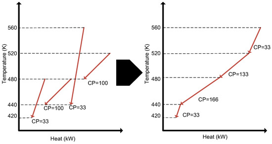
Figure 1.
Composite curves.
The most efficient thermal power generation process is the Carnot cycle, which is a basic element of this work and will be used to determine the maximum theoretical power generation from the heat sources. The Carnot cycle consists of four steps, i.e., isothermal heat addition from a heat source at temperature TH, isentropic expansion, isothermal heat removal into a heat sink at temperature TL, and isentropic compression. In order for power to be generated in the cycle, TH needs to be greater than TL. The Carnot cycle assumes that there is no energy lost due to friction, no exchange of heat between various parts of the engine, and no transfer of heat from the cycle to the surrounding environment. The efficiency of the Carnot cycle can be calculated as
In the problem addressed in this work, heat is transferred from a composite heat source profile through Carnot cycles to a low temperature reservoir. In a given temperature interval j from Ti to Ti+1, the heat available from the source profile segment is given by
Equation (2) is applied for non-isothermal intervals where CPj is the heat capacity flowrate (kW/K) of the profile segment, Ti is the inlet temperature (K) and Ti+1 is the exit temperature (K) of the heat source composite after heat has been removed. The heat capacity flow rate is the product of the heat capacity and the flow rate of the stream. Equation (3) is applied for isothermal intervals where Hv,j is the latent heat (kW). For maximum power generation, the low temperature reservoir is assumed to be an isothermal utility at ambient temperature (TL) with an infinite heat capacity flow rate.
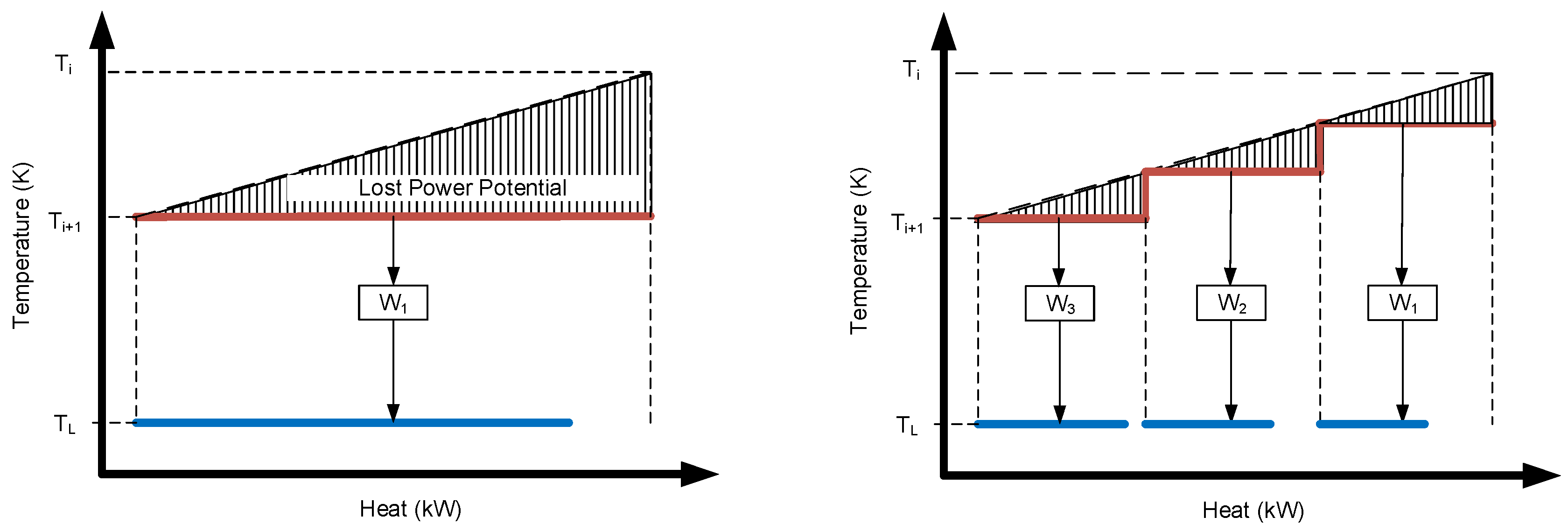
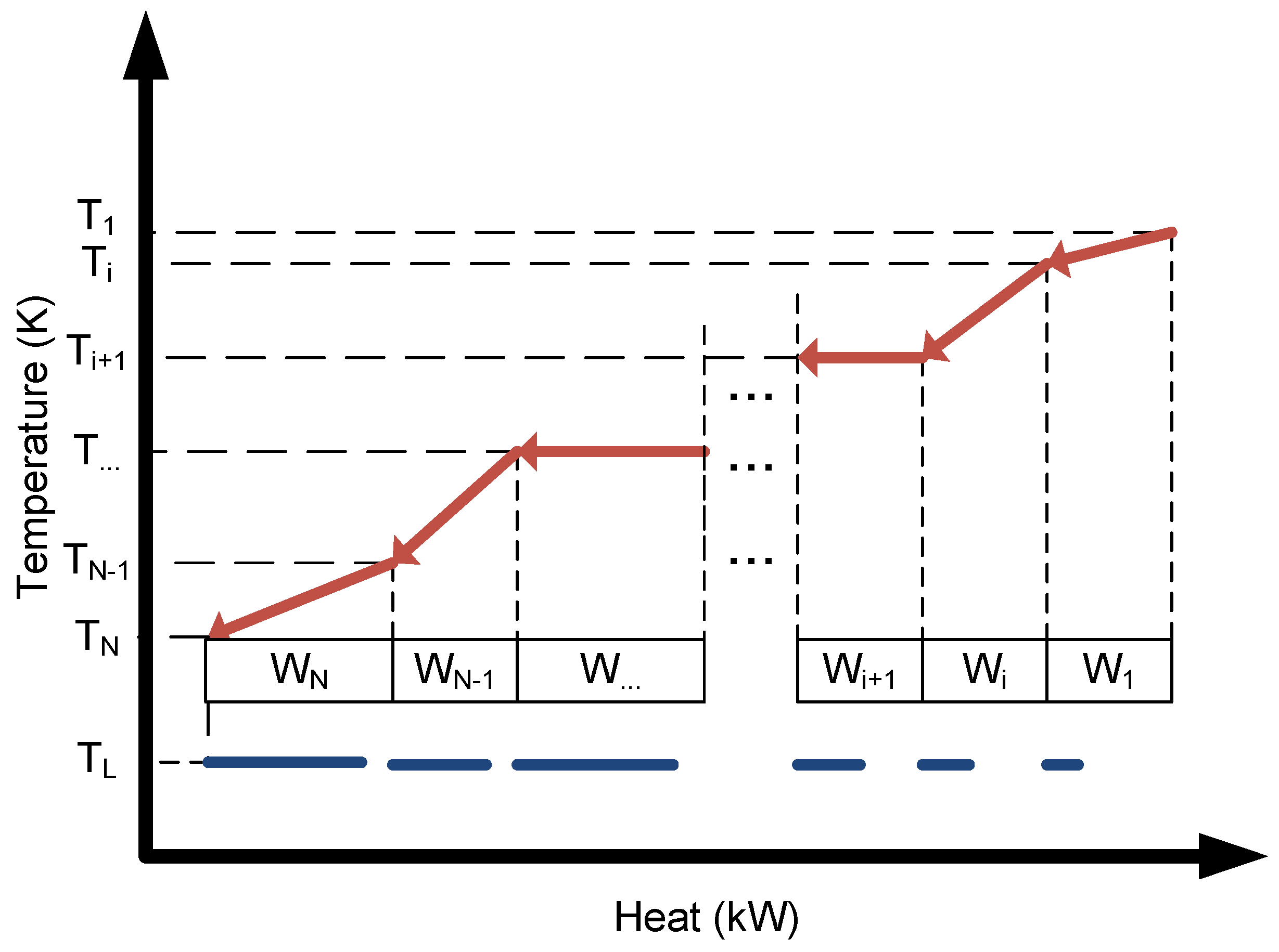
While the Carnot cycle assumes the heat source to be isothermal, a typical heat source composite segment is not isothermal. As a result, for a single Carnot cycle, the hot reservoir would take the lowest source temperature in the temperature interval as illustrated in Figure 2, i.e., TH = Ti+1. This will forfeit power generation potential and therefore present a lost opportunity for power generation. To increase power generation from the heat source profile, multiple Carnot cycles can be deployed, as illustrated in Figure 3. As the number of cycles approaches infinity, the hot temperature reservoirs of the Carnot cycles will approach the heat source profile and power generation will be maximized.
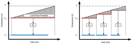
Figure 2.
Power potential lost for different number of carnot cycles.
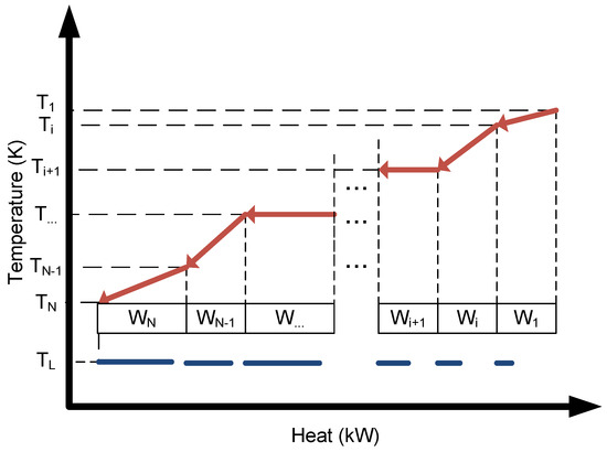
Figure 3.
Interval analysis composite curve.
Over an infinitesimal temperature difference, the power that can be generated with a Carnot cycle is
The maximum amount of power from a generated from a non-isothermal heat source composite segment is determined via integration over the temperature range of the interval from Ti+1 to Ti
The analytical solution of Equation (6) is given by
Equation (6) can be used to find the maximum amount of power that can be generated and can be found in the literature [16,18,19].
For the special case of an isothermal interval with Ti+1 = Ti, the maximum work becomes:
Equation (6) is also known as availability. An alternative derivation of the equation is presented in Appendix A. Since heat flows are given from the T-H profiles and power generation needs to be determined, it is convenient to develop expressions for temperature interval power generation efficiencies. The efficiency for a non-isothermal interval and an isothermal interval are given by Equations (8) and (9):
In process energy integration (Pinch Analysis), the heat capacity is assumed to be constant due to relatively small variations over typical temperature ranges. If the heat capacity needs to be expressed as a function of temperature, numerical integration of Equation (5) can be performed to determine the maximum amount of power that can be generated from an interval.
This section presents an algebraic procedure to calculate the maximum amount of power generated from a heat source profile comprised of multiple streams. The procedure takes the form of a problem table algorithm and is similar in structure to approaches available for heat integration [7]. The maximum power generation can be quickly determined with the procedure, which involves only a few very quick calculations and can easily be completed in a spreadsheet.
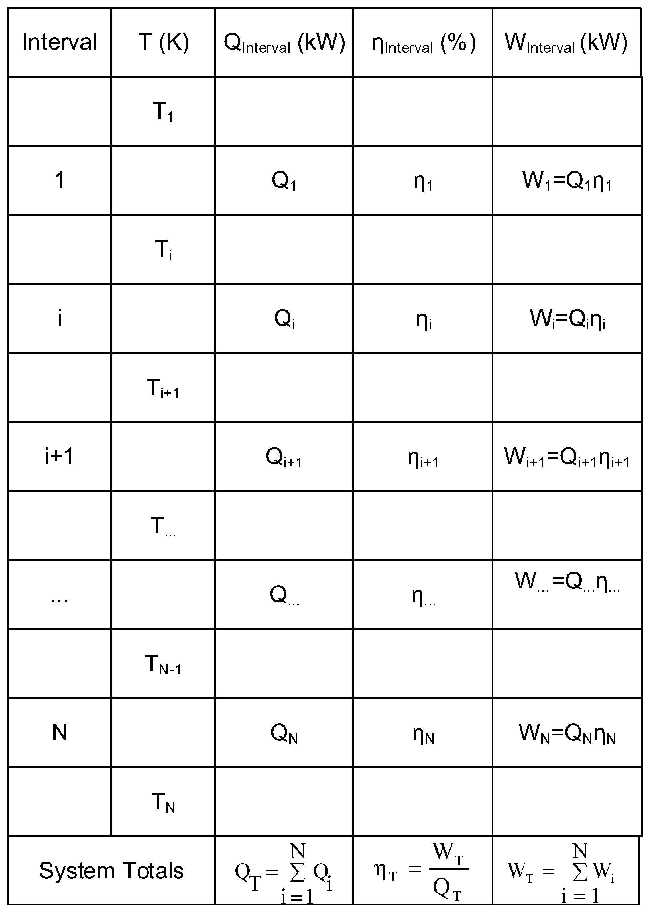
The problem table is constructed from high to low temperature and considers each temperature interval of the problem as a row. Temperature intervals are determined from the T-H composite profile (Figure 3). Starting from the highest temperature and moving towards lower temperatures, the first temperature interval ends and the next interval starts, when a change in the slope of the composite occurs, i.e., a change in the presence of individual streams that comprise the composite segments occurs. The intervals are traced until the lowest temperature of the T-H composite is reached. In terms of temperature data, the start/end temperature of each interval is recorded in the problem table. Figure 4 shows a schematic of a basic problem table in its general form with N temperature intervals corresponding to N + 1 temperature values. Each temperature interval is a row in the problem table, for which the following information is determined:
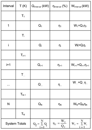
Figure 4.
Example problem table.
- (a)
- The heat transferred from the hot streams (or composite) present in the interval into the cycle is determined using Equation (2) in the case of a non-isothermal interval, or using Equation (3) in the case of an isothermal interval.
- (b)
- The interval power generation efficiency is determined using Equation (8) in the case of a non-isothermal interval, or using Equation (9) in the case of an isothermal interval.
- (c)
- The maximum amount of power that can be generated from the heat available in the interval is determined as the product of available heat from (a) and interval power generation efficiency from (b).
The above calculations are performed for all temperature intervals, yielding the maximum power that can be generated from each interval hot stream composite segment. The total amount of power for the entire set of streams comprising the composite is obtained as the sum of power generation over all intervals. Finally, we calculate the overall maximum theoretical (Carnot) efficiency of power generation from the set of heat source streams represented in the hot composite, i.e., over all N temperature intervals, as follows:
The cooling duty of the problem, i.e., the heat ejected from the hot streams for the initial case of no power generation, is reduced by the amount of power generated. This information may be useful to a designer interested in estimating possible reductions in cooling related footprints, e.g., cooling tower makeups or thermal pollution from marine discharges.
3. Results and Discussion
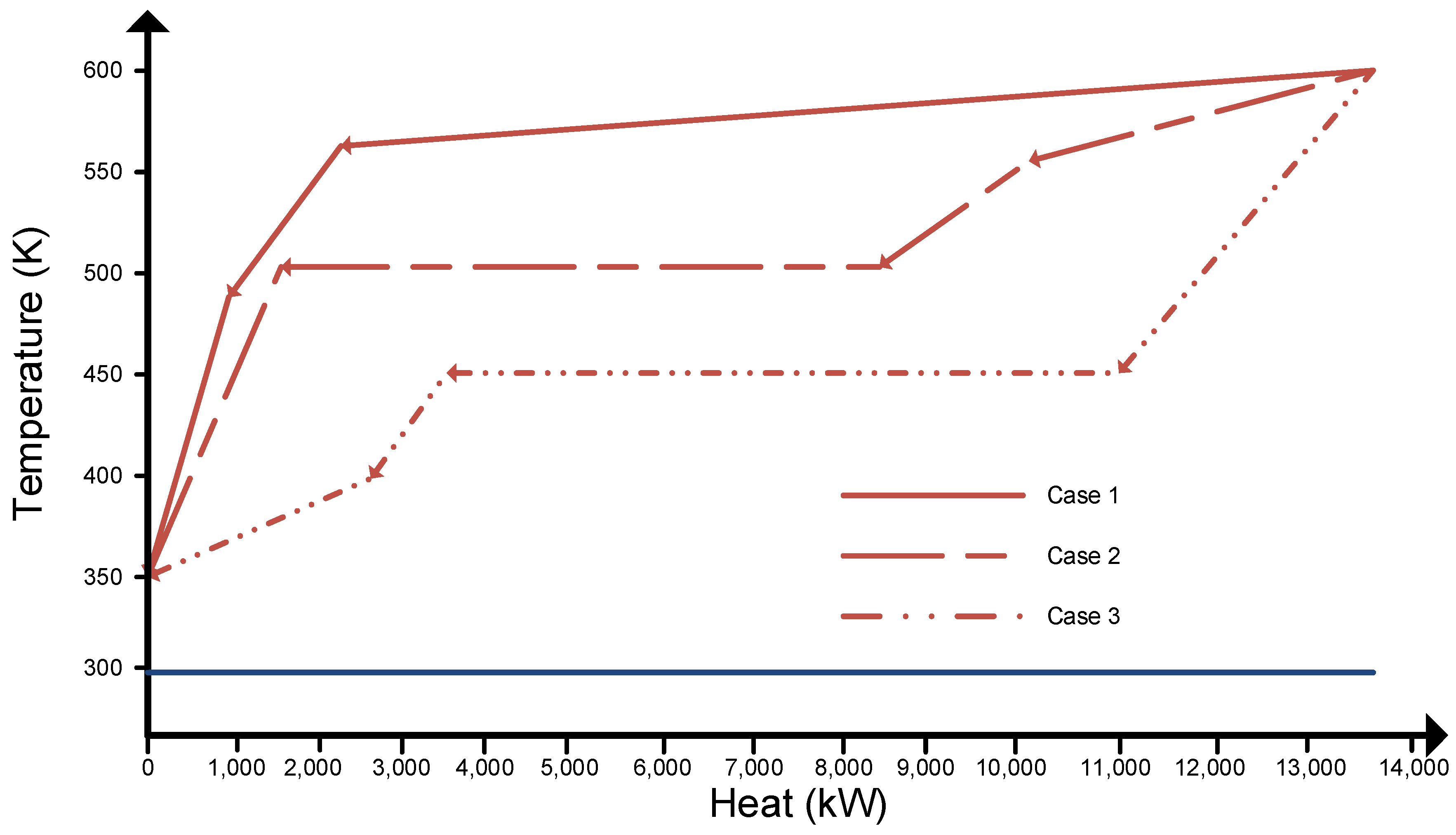
The targeting procedure is illustrated with three example cases, for which the hot composite curves are shown in Figure 5. The data for the individual streams that make up the hot composites are summarized in Table 1. The temperature of the low temperature reservoir is assumed to be 298 K for all cases. The total amount of heat that needs to be removed from the hot streams is identical for all three cases (13,700 kW). Similarly, the streams in all three cases operate within the same temperature range. This means that a single Carnot cycle with a hot reservoir temperature at the lower temperature of the range (350 K), would have an efficiency of 14.9% and produce the same amount of power (2035 kW) for all three cases.
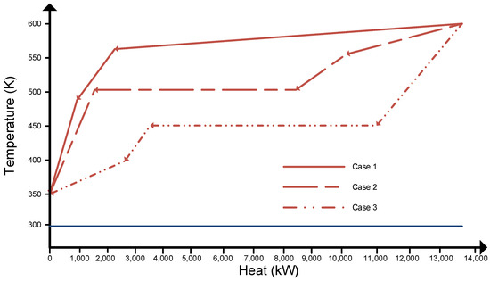
Figure 5.
Case study composite curves.

Table 1.
Streams Data for illustrative examples.
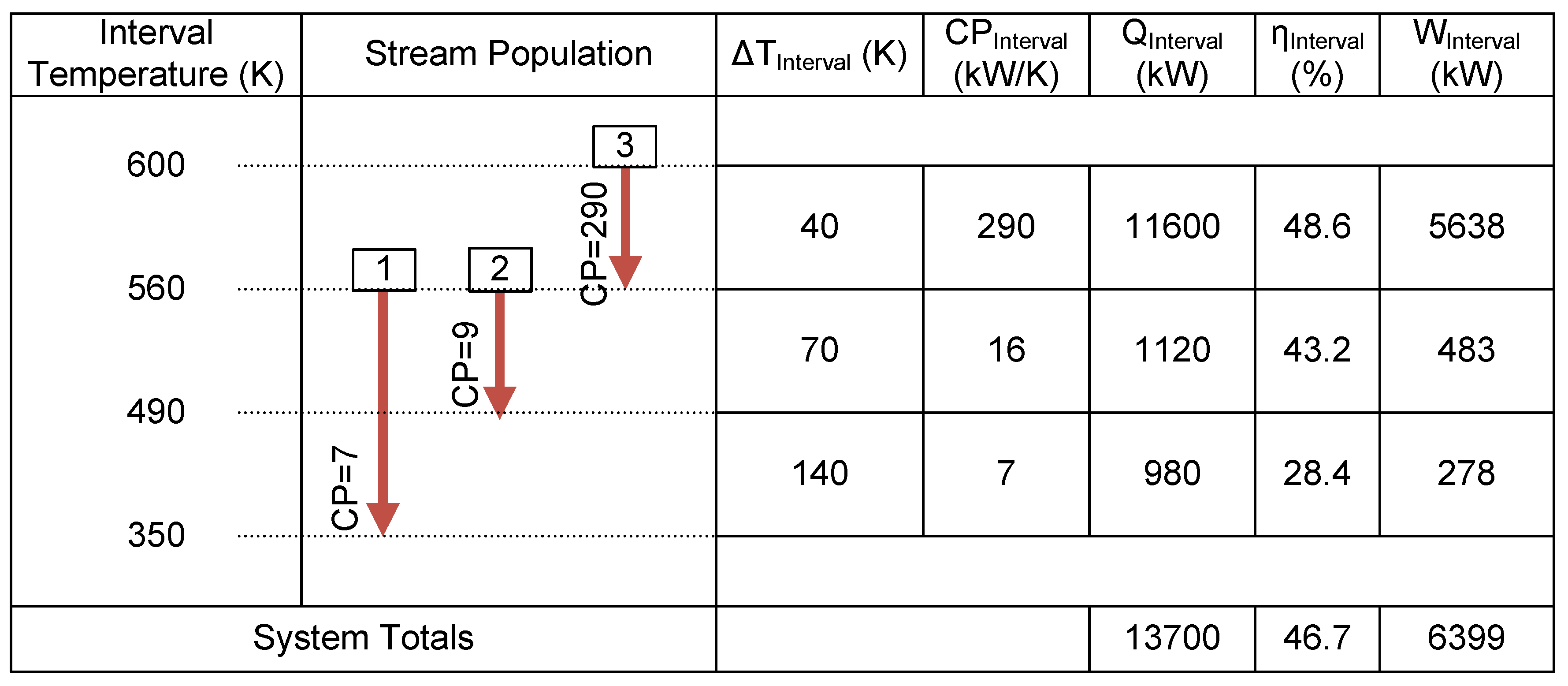
The problem table for each case was developed using the procedure outlined in the previous section. The problem table for Case 1 is shown in Figure 6. As can be seen from the data and composite curve for Case 1 (Table 1 and Figure 5), there are three changes in the streams that comprise the composite, resulting in three temperature intervals. All temperature intervals are non-isothermal and the heat removed from the composites is determined from Equation (2) for all three intervals. For instance, in the second interval, the combined heat capacity flow rate of the composite segment comprised by streams 1 and 2 is 16 kW/K and the interval ranges from 560 K to 490 K, i.e., has an interval temperature difference of 70 K. This results in a combined heat removal from the hot streams in the interval to be 1120 kW. Next, the interval efficiency for the non-isothermal interval is determined from Equation (8) using the interval temperatures:

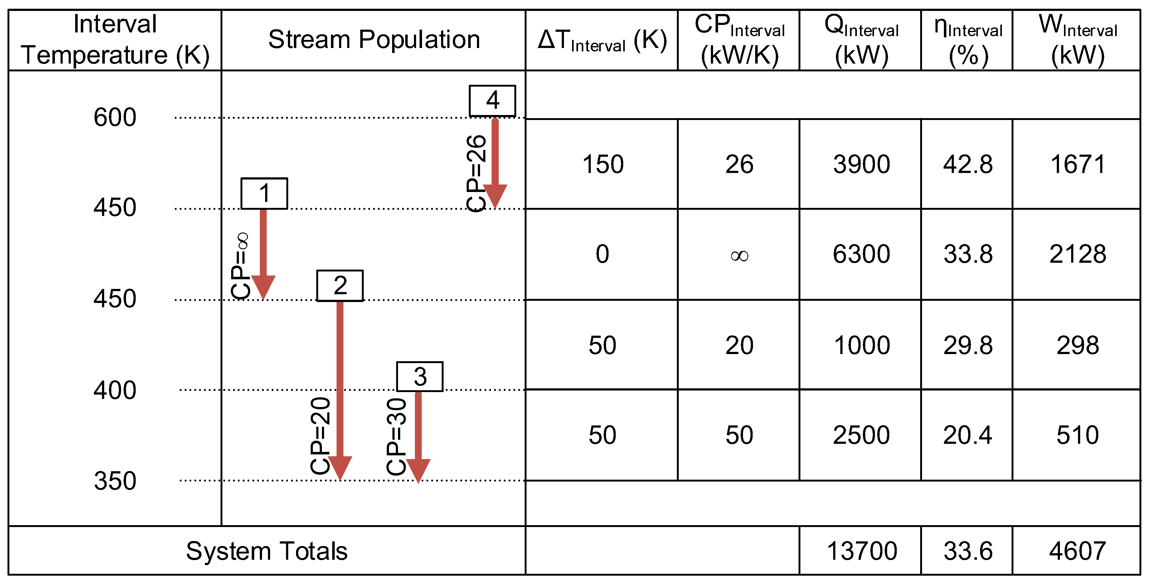
Figure 6.
Case study 1 problem table.
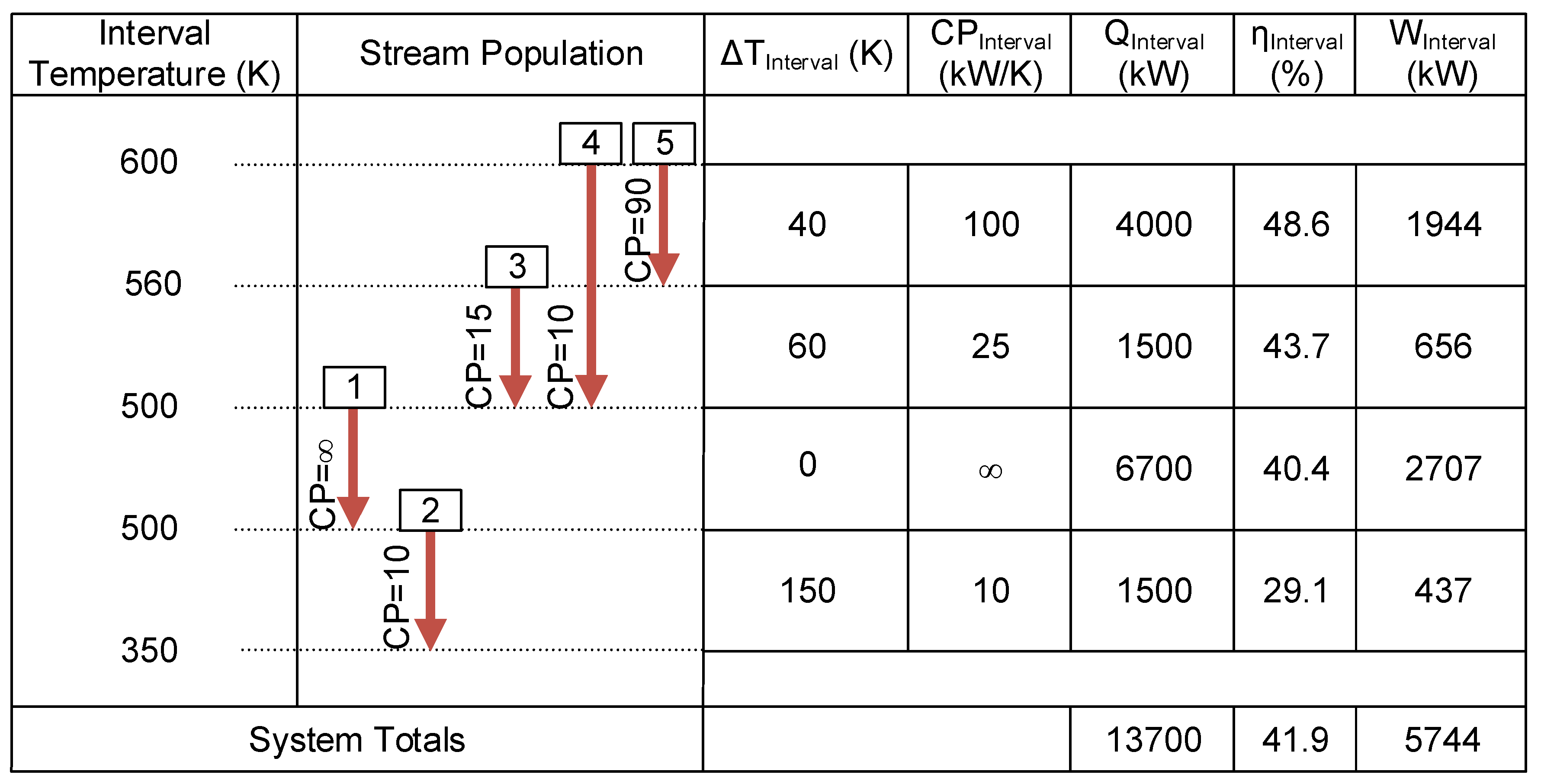
The resulting maximum power generation potential from the heat in the interval becomes 483 kW. These calculations are repeated for each interval and the totals are determined. Over all three intervals, Case 1 has the potential to produce a maximum of 6399 kW of power from the 13,700 kW of heat ejected from the streams, which results in an overall maximum power generation efficiency of 46.7%. The problem tables for Cases 2 and 3 are developed accordingly and shown in Figure 7 and Figure 8. The third temperature interval of Case 2 (Figure 7) and the second temperature interval of Case 3 (Figure 8) are isothermal with a heat capacity flow rate approaching infinity. The heat ejected from the hot streams in these intervals and the maximum power generation efficiency is determined using Equations (3) and (9), respectively. Comparing the three cases, Case 1 ejects most heat at higher temperatures (Figure 5), which results in the highest maximum theoretical work (6399 kW), followed by Case 2 (5744 kW) and Case 3 (4607 kW). This highlights the importance of developing case specific targets that consider the temperature vs. heat removal profiles of the multiple heat sources associated with a given problem.
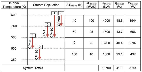
Figure 7.
Case study 2 problem table.

Figure 8.
Case study 3 problem table.
Another illustrative example will be presented to validate the proposed method against those in literature. Although this procedure is novel to calculate maximum power generation for a set of hot streams, it can be validated by the exergy targeting procedure used by Marmolejo-Correa and Gundersen [19]. As exergy is defined as the maximum power that can be generated, the maximum power generated using the proposed approach will be compared to the exergy target from Marmolejo-Correa and Gundersen’s exergy targeting procedure. Table 2 shows the streams that will be used in this illustrative example.
Table 2.
Validation case study.
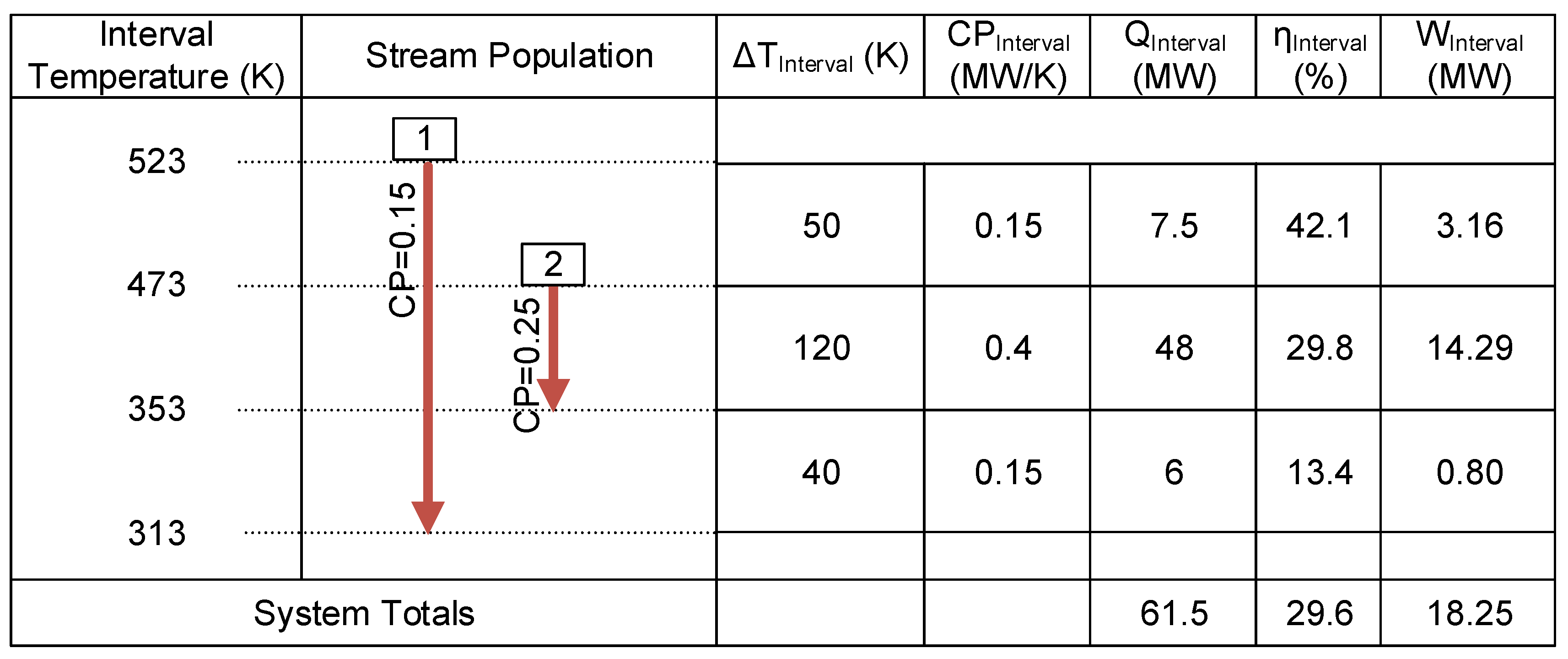
In this example, the temperature of the low temperature reservoir was 288 K. Figure 9 shows the problem table for the illustrative example.

Figure 9.
Validation case study problem table.
It was found that 18.25 MW of power can be generated from the two hot streams. Marmolejo-Correa and Gundersen found that the exergy of the two streams to be 18.25 MW. This confirms our results and validates the proposed procedure.
The procedure can be used to determine the maximum power generation potential (target) from composites of multiple heat source streams quickly and reliably without the need for intensive calculations. All three cases of the illustrative examples, regardless of the number of temperature intervals involved, could be solved from scratch in MS Excel in a few minutes, which makes the procedure practical and attractive to develop maximum power generation potentials (targets) from excess (process) heat for use in high-level screening studies in line with the process integration philosophy of developing targets before design.
4. Conclusions
In this paper, a procedure was proposed to determine the maximum amount of power that can be generated from a set of waste heat streams. The method was based on the Carnot efficiency and basic thermodynamic relationships between heat and power. The proposed procedure is similar in procedure to problem tables used in process integration. The procedure can be used to quickly calculate the theoretical maximum power generation to set a target for actual power generation. Three illustrative examples were used to show the simplicity of the procedure. Based on the targets, decisions can be taken to justify time for the development of specific power generation systems designs to generate power from the heat ejected from the multiple hot streams involve.
Acknowledgments
Patrick Linke, holder of the Qatar Shell Professorship for Energy and Environment, gratefully acknowledges funding received from Shell Qatar.
Author Contributions
This publication has resulted from research performed by Omar Al-Ani as graduate student under the guidance of Patrick Linke. Both authors contributed directly to all aspects of the work.
Conflicts of Interest
The authors declare no conflict of interest.
Nomenclature
| CPj | Heat capacity flow rate of hot composite in non-isothermal interval j |
| Hv,j | Latent heat of hot composite in isothermal interval j |
| Hi | Enthalpy of hot composite at interval inlet temperature |
| Hi+1 | Enthalpy of hot composite at interval exit temperature |
| Qj | Heat ejected from hot composite in interval j |
| Entropy generation in interval j | |
| Si | Entropy of hot composite at interval inlet temperature |
| Si+1 | Entropy of hot composite at interval exit temperature |
| Ti | Initial temperature of hot composite in interval j |
| Ti+1 | Final temperature of hot composite in interval j |
| TH | Temperature of the high temperature reservoir |
| TL | Temperature of the low temperature reservoir |
| T0 | Dead state temperature |
| Maximum theoretical power generation in interval j | |
| Maximum power generation efficiency in interval j | |
| Maximum power generation efficiency across all temperature intervals | |
| Ψ | Availability |
Appendix A
This Appendix presents an alternative derivation of Equation (10) to determine the maximum theoretical work from a composite segment in a temperature interval [20]. The steady state energy and entropy balances for interval j are given by:
Combining Equations (A1) and (A2) yields
The entropy generated from the system () will be zero as all stages in the Carnot cycle are reversible. Hence, the maximum amount of work that can be generated is
Equation (A5) is known as availability (), i.e., the maximum work output associated with any steady state process:
Using partial derivatives, the relationship between the availability and temperature at constant pressure can be determined for interval j.
Integration of Equation (A6) determines yields
Equations (6) and (A10) are equivalent, i.e., the difference in availability equals the work obtained from an infinite number of Carnot cycles.
References
- Oluleye, G.; Jobson, M.; Smith, R. A hierarchical approach for evaluating and selecting waste heat utilization opportunities. Energy 2015, 90, 5–23. [Google Scholar] [CrossRef]
- Öhman, H.; Lundqvist, P. Comparison and analysis of performance using Low Temperature Power Cycles. Appl. Therm. Eng. 2013, 52, 160–169. [Google Scholar] [CrossRef]
- Minea, V. Power generation with ORC machines using low-grade waste heat or renewable energy. Appl. Therm. Eng. 2014, 69, 143–154. [Google Scholar] [CrossRef]
- Tchanche, B.F.; Lambrinos, G.; Frangoudakis, A.; Papadakis, G. Low-grade heat conversion into power using organic Rankine cycles—A review of various applications. Renew. Sustain. Energy Rev. 2011, 15, 3963–3979. [Google Scholar] [CrossRef]
- Linnhoff, B. Thermodynamic Analysis in the Design of Process Networks. Comput. Chem. Eng. 1979, 3, 283–291. [Google Scholar] [CrossRef]
- Dhole, V.R.; Linnhoff, B. Total site targets for fuel co-generation, emissions, and cooling. Comput. Chem. Eng. 1993, 17, 101–109. [Google Scholar] [CrossRef]
- El-Halwagi, M.M. Sustainable Design through Process Integration; Elsevier: Amsterdam, The Netherlands, 2012; pp. 1–14. [Google Scholar] [CrossRef]
- Hackl, R.; Andersson, E.; Harvey, S. Targeting for energy efficiency and improved energy collaboration between different companies using total site analysis (TSA). Energy 2011, 36, 4609–4615. [Google Scholar] [CrossRef]
- Bungener, S.; Hackl, R.; Van Eetvelde, G.; Harvey, S.; Marechal, F. Multi-period analysis of heat integration measures in industrial clusters. Energy 2015, 93, 220–234. [Google Scholar] [CrossRef]
- Marechal, F.; Kalitventzeff, B. Targeting the integration of multi-period utility systems for site scale process integration. Appl. Therm. Eng. 2003, 23, 1763–1784. [Google Scholar] [CrossRef]
- Stijepovic, V.Z.; Linke, P.; Stijepovic, M.Z.; Kijevčanin, M.L.J.; Šerbanović, S. Targeting and design of industrial zone waste heat reuse for combined heat and power generation. Energy 2012, 47, 302–313. [Google Scholar] [CrossRef]
- Linnhoff, B.; Dhole, V.R. Shaftwork targets for low-temperature process design. Chem. Eng. Sci. 1992, 47, 2081–2091. [Google Scholar] [CrossRef]
- Mavromatis, S.P.; Kokossis, A.C. Conceptual optimisation of utility networks for operational variations—I. Targets and level optimisation. Chem. Eng. Sci. 1998, 53, 1585–1608. [Google Scholar] [CrossRef]
- El-Halwagi, M.; Harell, D.; Dennis Spriggs, H. Targeting cogeneration and waste utilization through process integration. Appl. Energy 2009, 86, 880–887. [Google Scholar] [CrossRef]
- Curzon, F.L. Efficiency of a Carnot engine at maximum power output. Am. J. Phys. 1975, 43, 22. [Google Scholar] [CrossRef]
- Ondrechen, M.J.; Andresen, B.; Mozurkewich, M.; Berry, R.S. Maximum work from a finite reservoir by sequential Carnot cycles. Am. J. Phys. 1981, 49, 681–685. [Google Scholar] [CrossRef]
- Ibrahim, O.M.; Klein, S.A.; Mitchell, J.W. Optimum Heat Power Cycles for Specified Boundary Conditions. J. Eng. Gas Turbines Power 1991, 113, 514–521. [Google Scholar] [CrossRef]
- Park, H.; Kim, M.S. Thermodynamic performance analysis of sequential Carnot cycles using heat sources with finite heat capacity. Energy 2014, 68, 592–598. [Google Scholar] [CrossRef]
- Marmolejo-Correa, D.; Gundersen, T. New graphical representation of exergy applied to low temperature process design. Ind. Eng. Chem. Res. 2013, 52, 7145–7156. [Google Scholar] [CrossRef]
- Sandler, S.I. Chemical, Biochemical, and Engineering Thermodynamics; John Wiley & Sons: New York, NY, USA, 2006; Volume A5. [Google Scholar]

© 2018 by the authors. Licensee MDPI, Basel, Switzerland. This article is an open access article distributed under the terms and conditions of the Creative Commons Attribution (CC BY) license (http://creativecommons.org/licenses/by/4.0/).