A Traveling-Wave-Based Fault Location Scheme for MMC-Based Multi-Terminal DC Grids

Abstract

This paper presents a novel fault location scheme of DC line in modular multilevel converter (MMC)-based multi-terminal DC (MTDC) grids. Considering the low-inertia characteristics and the meshed topology, the scheme, based on traveling-wave principle, is divided into three steps, namely, faulty pole identification, faulty segment determination and fault-distance calculation. With accurate amplitude, polarities and arrival times of the first arrival current traveling waves (FACTWs) collected from time-synchronized measurements taken just at the converter stations, the proposed scheme can correctly determine the faulty pole, the faulty segment and the precise fault location. The continuous wavelet transform (CWT) is deployed to extract the required features of the input signals at the DC lines. Since the scheme merely needs the features of FACTWs, the practical difficulties of detecting subsequent traveling waves are avoided. A four-terminal MMC-based high voltage direct current (HVDC) grid was built in PSCAD/EMTDC software to evaluate the performance of the fault-location scheme. Simulation results for different cases demonstrate that the proposed fault-location scheme has high accuracy, good adaptability and reliability. Furthermore, the algorithm can be used for a MMC-MTDC grid with any number of meshes.

1. Introduction

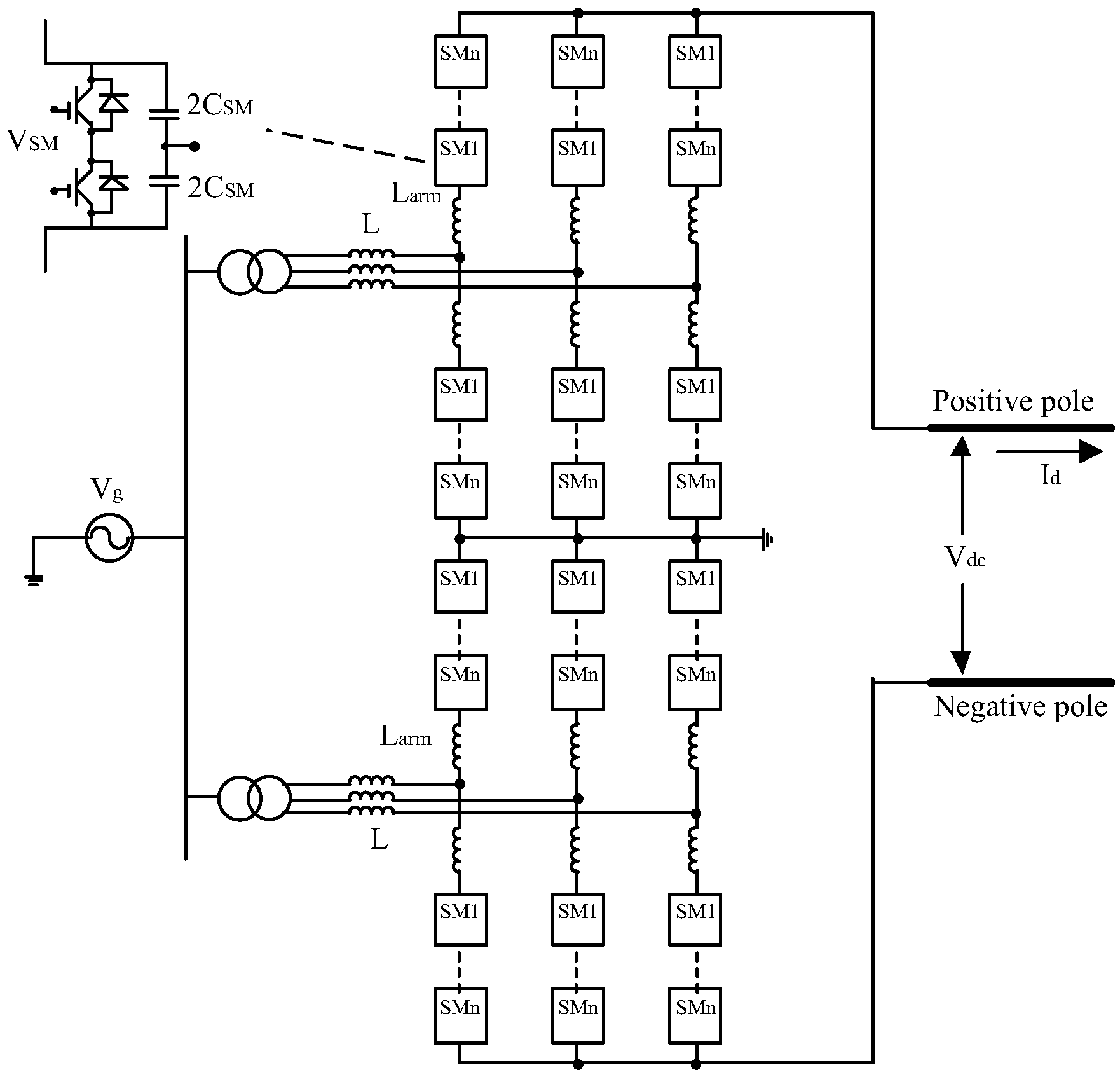
Voltage source converter (VSC)-based high voltage direct current (HVDC) technology has become a focus for scholars all over the world, because the technology has the advantages of controlling active and reactive power independently, reversing power flow without changing voltage polarity, supplying power for passive networks, etc. [1,2]. The main topologies of VSC include two-level and three-level VSC and modular multilevel converter (MMC). Since MMC has the advantages of higher quality of output waveform, lower switching frequency and power loss and higher reliability, it has been regarded as an excellent choice for bulk power transmission, especially for multi-terminal direct current (MTDC) grid.

At present, the VSC-HVDC projects that have been put into operation mainly include point-to-point and multi-terminal transmission projects, such as Gotland point-to-point two-level VSC-based HVDC project, Nan’ao three-terminal and Zhoushan five-terminal MMC-based DC transmission projects [3,4], but they all do not form a DC grid. Zhangbei MMC-based HVDC project will build China’s first VSC-based HVDC grid, which is still in the preparatory stage [5].

Compared with MTDC transmission project, the biggest advantage of MTDC grid is that there are multiple transmission lines between converter stations to form mesh structures and increase system redundancy, which significantly improves power supply reliability, decreases the number of converter stations and reduces investment and operation costs [6,7]. However, due to the use of long-distance lines for power transmission, the MTDC power grid is fault-prone, and the failure of any line may cause the electrical quantities of all lines to be influenced. In addition, due to varied topography and long distance, after the occurrence of a line fault, artificial line patrol is difficult to find the fault point, which results in greatly delay of the fault recovery time. In order to relief the burden of patrol personnel, shorten the fault recovery time and reduce the revenue losses due to power outage, choosing reliable algorithms of fault location has important theoretical significance and engineering application value.

The fault location methods of high-voltage alternating current (HVAC) power networks are by far relatively mature, and mainly include two categories [8,9,10,11]: impedance-measurement method and traveling-wave-based method. In the former method, postfault voltages and currents of HVAC systems within the first several milliseconds are used to calculate the impedance to pinpoint the exact fault location. However, for MMC-HVDC systems, the impedance calculation may not be easy, due to the low-inertia characteristics and the application of fast-acting protection devices. Compared to the impedance-measurement method, as a result of merely utilizing the fault-generated surge, a shorter data window is required in the traveling-wave method. Furthermore, the amplitude and polarity of the traveling wave will not be affected by the fault inception instant in DC systems, which is different from AC systems. Therefore, the traveling-wave-based method is very suitable for DC systems, hence, the proposed method is based on the traveling-wave principle.

The fault location method based on the distributed parameter model proposed in [12] has a good applicability to the two-terminal MMC-HVDC transmission line, and the accuracy of fault location is high, but it is difficult to extend to the multi-terminal MMC-based MTDC grid. In [13,14], two fault location methods based on natural frequency of the traveling wave are presented. Although the two methods avoid the identification of the traveling wave front, there are problems such that the equivalent impedance of the measuring terminal is difficult to obtain accurately and the faulty branch of the multi-terminal system is difficult to select. In [15], a one-terminal fault location method based on parameter identification principle is proposed, but this method is just applicable to the case where there are large capacitors in parallel at both ends of the transmission line. In [16], a fault location method combining wavelet transform (WT) with artificial neural network (ANN) algorithm is proposed. This method needs to set up many parameters for training neural network, and it takes a long time to learn to achieve sufficient location accuracy. A fault location method for multi-terminal VSC-HVDC system is proposed in [17]. In [18], a protection method based on wavelet modulus maxima of traveling waves is proposed for the point-to-point HVDC system. The method leads to a fast and reliable solution for the protection of HVDC lines. Besides, it is able to figure out the exact fault location. The method uses both voltage and current measurements obtained at the converter stations to identify the faulty line for protection purposes. However, it cannot figure out the exact fault location. So far, there are few fault location methods for multi-terminal MMC-HVDC grids reported in the literature.

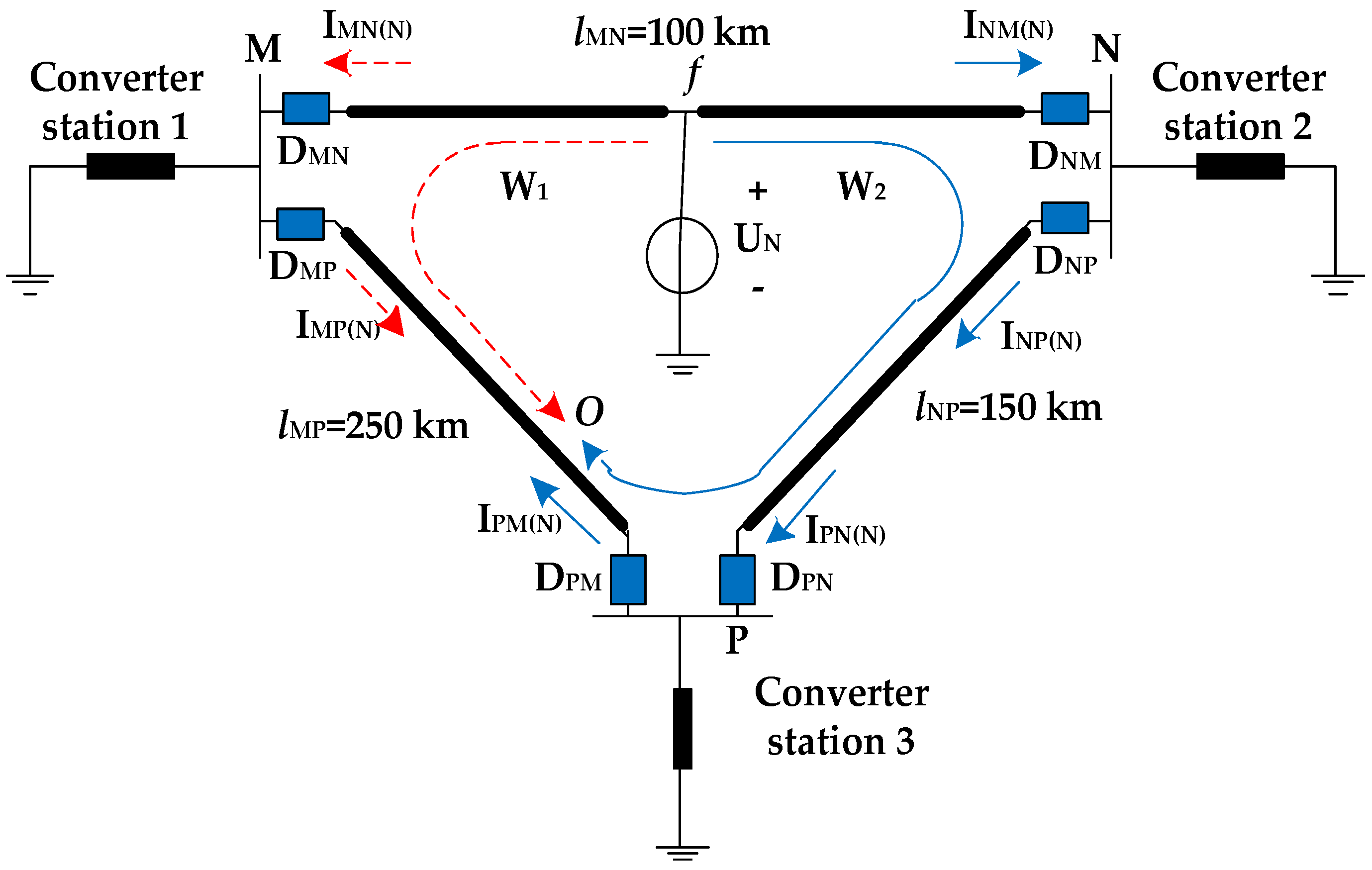
In this paper, a precise fault location scheme is introduced. The scheme utilizes the characteristics of the first arrival current traveling wave (FACTW), which are extracted and quantified by CWT, to realize fault location. Although this scheme is initially derived from a meshed three-terminal DC grid, it can be extended to a MMC-MTDC grid with any number of meshes.

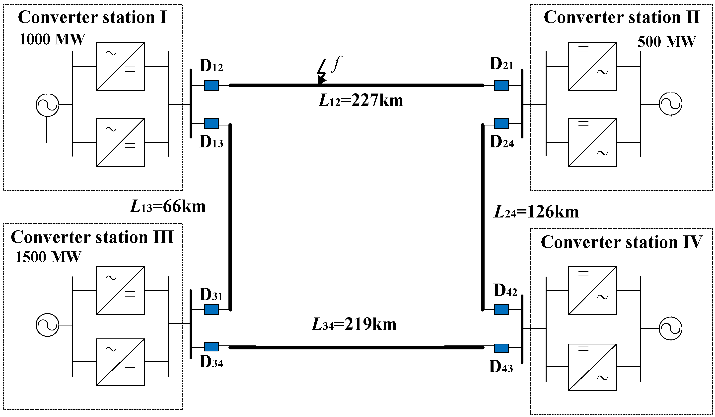
The remainder of paper is arranged as follows. The fault characteristic analysis is performed in Section 2. According to the conclusions of Section 2, Section 3 constructs the faulty pole identification criterion and faulty segment determination criterion, respectively, and, proposes the fault location algorithm. Based on the design parameters of Zhangbei ±500 kV four-terminal MMC-HVDC power grid in China, a simulation model was constructed to verify reliability and accuracy of the proposed fault-location scheme in Section 4 and the conclusions was drawn in Section 5.

2. Analysis of Fault Characteristics

2.1. Wavelet Analysis Theory

The fault traveling wave is essentially a non-stationary high-frequency signal. The wavelet transform has the ability to represent the local characteristics of a signal in the time domain and frequency domain, so it is very suitable for analyzing the fault traveling wave signals and extracting their features [19].

The continuous wavelet transform (CWT) of a signal f(x) is written as follows:

$$\mathrm{CWT}(f(x);a,b)={\displaystyle \underset{-\infty }{\overset{+\infty }{\int }}f(x)}{\psi }_{a,b}^{*}(x)dx$$

(1)

$${\psi }_{a,b}^{*}(x)=\frac{1}{\sqrt{a}}\psi (\frac{x-b}{a})$$

(2)

where Ψ_a,b(x) is the mother wavelet, which is a continuous function. “a” is the scaling factor and “b” is the shifting.

Assuming that the wavelet coefficient of f(x) at each scale s is $W_s^d$f(x). If the function

$$\left|W_s^{d}f(x)\right|\le \left|W_s^{d}f(x_n)\right|$$

(3)

is satisfied for all x in the neighborhood of x_n under scale s, the modulus maximum point of WT is x_n, and the modulus maximum of WT is $W_s^d$f(x_n).

In the actual computation of wavelet modulus maxima points, the wavelet coefficients of traveling waves were first be calculated through the program. Then, the modulus of each wavelet coefficient is calculated. Finally, the wavelet modulus maxima points were obtained by comparing the modulus of wavelet coefficients of several adjacent points.

The singularity detection theory shows that there is a one-to-one correspondence between the modulus maximum of CWT and the abrupt point of the signal [20]. Therefore, it is feasible to use the CWT modulus maximum of the measured-line current to detect the surge arrival time. Besides, the sign and the absolute value of the CWT modulus maximum indicate mutant polarity and intensity of the input signal, respectively. Thus, the modulus maximum of CWT is applied to the proposed fault-location scheme.

2.2. Fault Traveling Wave Polarity Analysis

The MMC-MTDC grid is a bipolar system, which contains many lines, and the fault types include monopolar grounding fault and bipolar short-circuit fault. The symmetric bipole topology of MMC is shown in Figure 1. Therefore, before calculating the fault distance, it is necessary to select the faulted segment and the faulted pole. In this paper, on the basis of the traditional traveling-wave-polarity principle for AC systems [21], a novel traveling-wave-polarity principle is proposed considering the specificity of the MMC-MTDC grid. To begin with, the traditional principle is introduced.

2.2.1. Introduction of Traditional Traveling-Wave-Polarity Principle

Take the two-terminal AC transmission system shown in Figure 2 as an example. The fault points f₁ and f₂ respectively indicate the internal and external faults for the line MN. The positive direction of current is specified as from the bus to the line. The following analysis is based on a single-phase system for convenience.

According to the traveling-wave theory [10], when a fault occurs on the transmission line, it is equivalent to superimposing an additional voltage source at the fault point. Under the effect of the additional source, traveling waves are generated and propagate along the line from the fault point to both terminals.

Figure 3 shows the superimposed circuits of the internal fault f₁ and the external fault f₂. The red solid arrows are the polarities of FACTWs while voltage of the additional source is negative, and the blue dotted arrows are the polarities of FACTWs while voltage of the additional source is positive. In Figure 3, assume that the postfault voltage on the fault point is V_F = U_m sin(wt + θ), the voltage of the additional source will be −V_F, which varies with the change of the fault inception angle. If the fault inception angle is in the range of 0° to 180°, the voltage of the additional source will be negative, otherwise it will be positive.

When an internal grounding fault occurs at f₁ for the line MN, the superimposed circuit of Figure 1 is illustrated as Figure 3a. It can be seen from Figure 3a, that after the occurrence of the fault, no matter whether the additional voltage source is positive or negative, polarities of FACTWs detected at both ends of the line MN are both the same.

For an external ground fault occurring at f₂, the line MN is normal and Figure 3b illustrates the superimposed circuit of Figure 2. As shown in Figure 3b, polarities of FACTWs detected at both terminals of the line MN are opposite to each other in any circumstance.

2.2.2. Polarity Analysis of FACTW for MMC-MTDC Grid

As mentioned earlier, the additional voltage source varies with different fault inception angles in AC systems. However, in DC systems, the additional source will always be same and has nothing to do with the fault time, since the voltage of the line is constant.

Without loss of generality, a three-terminal MTDC grid in Figure 4 is taken as an example. The voltage of the grid is −U_N. The length of each line is shown in Figure 4 and assuming that the lines all have the same parameters so that the traveling-wave propagation velocity of each line is equal. The positive direction of current is defined as from the bus to the line. The following analysis is based on a single-pole system for convenience.

As shown in Figure 4, the fault point is in the middle of the line MN. The FACTWs detected by the fault-location device D_ij at both ends of each line can be expressed by I_ij (i,j = M, N, P).

When the fault occurs, the FACTW W₁ and W₂ propagate from the fault point f to both sides of the line MN, and then propagate into other lines. The path of the FACTW, which is detected for the first time, is the shortest path between the fault point and the detector. As shown in Figure 4, the total length of all the lines in the meshed network is 800 km. Considering the same traveling-wave propagation velocities of each line, the current traveling wave W₁ and W₂ respectively propagate 400 km in different directions before they encounter each other at the O point shown in Figure 4, where is 100 km from the bus P. Before encountering, the propagation path of W₁ is the fault point f—the left half of the line MN—the bus M—the line MO, while the propagation path of W₂ is the fault point f—the right half of the line MN—the bus N—the line NP—the bus P—the line PO.

As the pre-fault voltage is −U_N, the voltage of the additional source is +U_N. From Figure 4, polarities of FACTWs detected by D_PN and D_NP are opposite to each other, but polarities of FACTWs detected by D_MN and D_NM as well as those detected by D_MP and D_PM are all identical to each other, respectively. Therefore, the faulted segment cannot be correctly identified only by judging whether the polarities of FACTWs at both terminals of the line are identical or not, so additional criterion need to be introduced.

As shown in Figure 4, further research found that although polarities of FACTWs at both ends of the faulty line MN and the healthy line MP are the same respectively, those of the line MN are all positive while those of the line MP are all negative.

The polarity characteristics analyzed above are based on a single-pole system, which are equal to the condition of negative-pole-ground fault in a bipolar system. The polarity characteristics of the positive-pole-ground fault can be obtained by the same way.

Therefore, for a bipolar MMC-MTDC power grid, the following conclusions are drawn:

• For a positive-pole grounding fault or a bipolar short-circuit fault, polarities of FACTWs at both terminals of the positive line in the faulted segment are all positive, while those in the non-fault segment are opposite to each other or all negative.
• For a negative-pole grounding fault or a bipolar short-circuit fault, polarities of FACTWs at both terminals of the negative line in the faulted segment are all negative, while those in the non-fault segment are opposite to each other or all positive.

2.2.3. Characteristic Analysis of Fault-Pole Line and Normal-Pole Line

The aforementioned analysis is based on a single-pole system. Accordingly, for the bipolar DC system, the faulty pole is necessary to be identified so that FACTWs of each fault-pole line can be used for following calculation.

In bipolar MMC-MTDC grids, when a monopolar fault occurs on the DC line, the abrupt current signal of the fault-pole line can be coupled to the normal-pole line. However, the current mutant intensity of the normal-pole line is much smaller than that of the fault-pole line. As a result, the amplitude of FACTW of the normal-pole line is obviously smaller than that of the fault-pole line, as shown in Figure 5.

For the bipolar short-circuit fault, since the fault both occurs on the positive line and the negative line, the amplitude of FACTWs of bipolar lines is equal to each other in theory, as shown in Figure 6.

3. Fault Location Scheme

3.1. Fault-Pole Identification Criterion

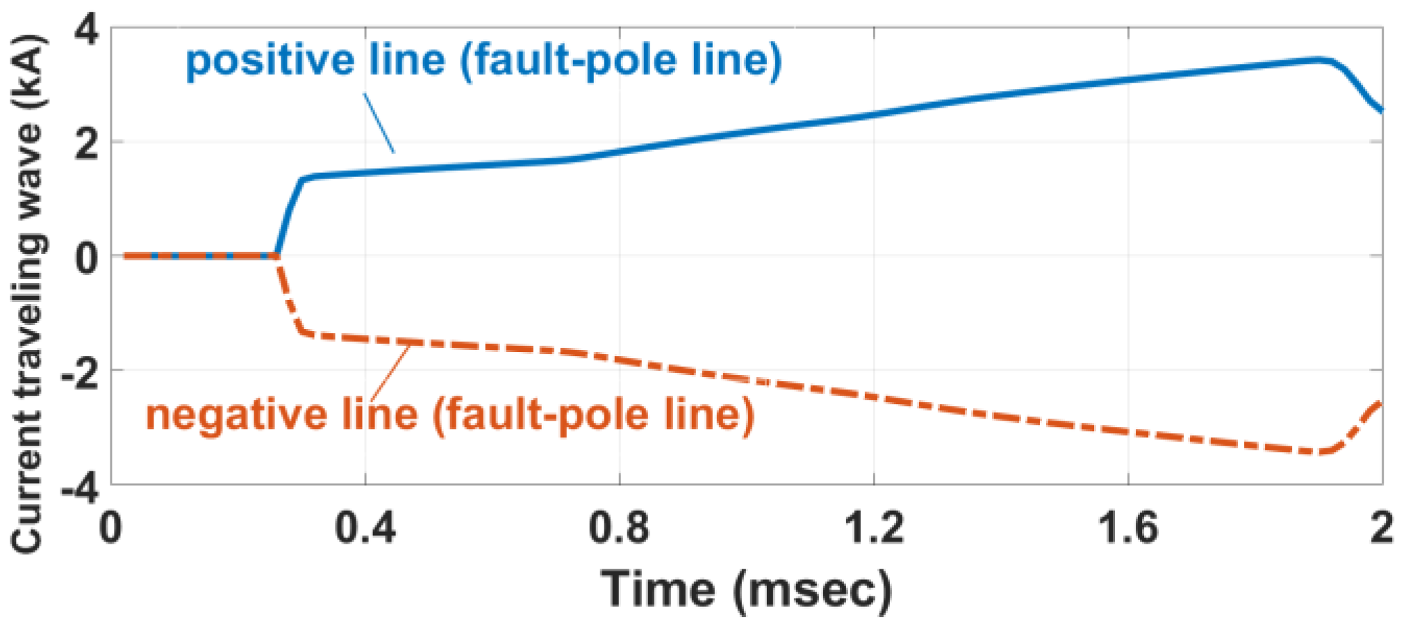
On the basis of the characteristic analysis in Section 2.2.3, the identification of faulty pole can be achieved by comparing the amplitude of FACTWs at the same terminals of each segment. According to the wavelet analysis theory in Section 2.1, the amplitude of FACTW can be approximately represented by the CWT modulus maximum.

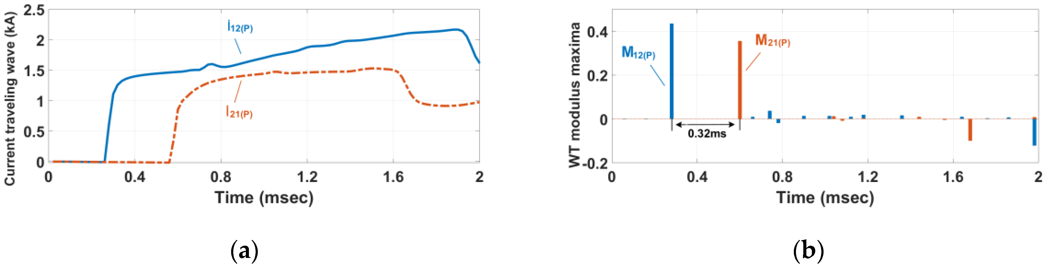
First, the following ratio is defined for convenience:

$${\lambda }_i=\left|\frac{M_{ij\left(P\right)}}{M_{ij\left(N\right)}}\right|$$

(4)

where M_ij(P) and M_ij(N) respectively denote the WT modulus maxima of the positive line and the negative line at i-terminal of the segment ij.

Then the fault-pole identification criterion can be constructed as follows: $1-k<{\lambda }_i<1+k$

$${\lambda }_i>1+k$$

(5)

$${\lambda }_i<1-k$$

(6)

$$1-k<{\lambda }_i<1+k$$

(7)

where k (0 < k < 1) denotes the reliable coefficient.

If (5) is satisfied, the positive pole is identified as the faulty pole; If (6) is met, the negative pole is identified as the faulty pole; If (7) is satisfied, the bipolar short-circuit fault is determined.

In order to ensure the reliability of the criterion and to avoid the frequent start of the fault-location device caused by noises, the validity of data used for the algorithm is needed to be verified. The verification criterion of data validation is as follows:

$$\Delta I_i>I_{set}$$

(8)

$$\Delta I_i=I_i-I_N$$

(9)

The value of the threshold I_set is defined as

$$I_{set}=K_{rel}{I}_N$$

(10)

where ΔI_i is the fault component current at ith sampling point. Ii denotes the instantaneous value of current at ith sampling point; K_rel denotes the reliable coefficient, whose value is 0.1 in this paper to avoid the influence of noises, and I_N denotes the rated current of each line; and the fault-location device starts if (10) is met for three consecutive samples.

3.2. Fault-Segment Determination Criterion

For the MMC-MTDC grid, after identifying the faulty pole, it is necessary to select the faulty segment correctly so as to calculate the fault distance accurately.

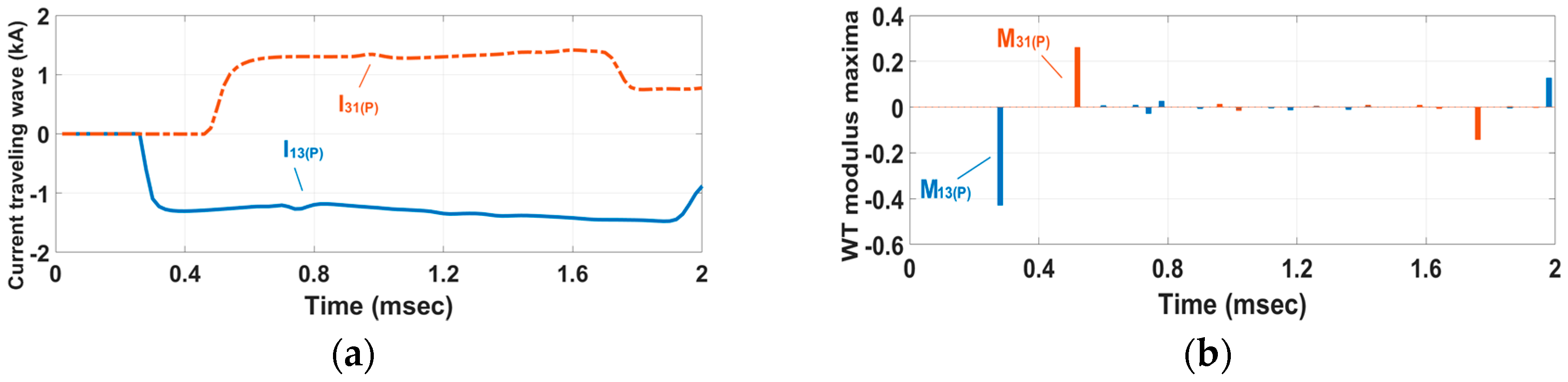
Based on the analysis in Section 2.2.1 and Section 2.2.2, the following faulty segment determination criterion can be constructed by using WT modulus maxima:

$$\{\begin{array}{l}{M}_{ij\left(P\right)}>0\\ M_{ji\left(P\right)}>0\end{array}$$

(11)

$$\{\begin{array}{l}{M}_{ij\left(N\right)}<0\\ M_{ji\left(N\right)}<0\end{array}$$

(12)

where M_ji(P) and M_ji(N) denote the WT modulus maxima of the positive and the negative line at j-terminal of the segment ij, respectively.

If the faulty pole is identified as positive pole, meanwhile (11) is met, the segment ij is determined as the faulted segment, otherwise the segment ij is verified as the non-fault segment; If negative pole is the faulty pole, and (12) is satisfied, the segment ij is judged as the faulted segment, otherwise the segment ij is healthy; For the bipolar short-circuit fault, in order to simplify calculation, the segment ij is selected as the faulted segment only need to satisfy (11).

3.3. Fault-Distance Calculation

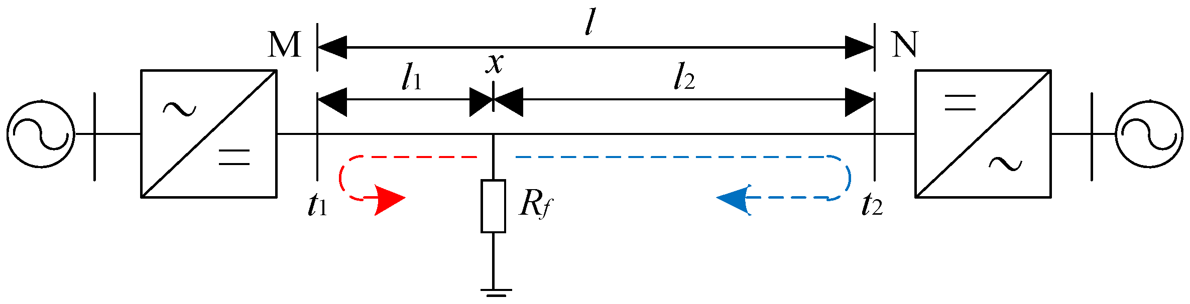
Once the faulted segment is determined, the fault distance will be further calculated. According to the traveling-wave principle, after a fault occurring on the transmission line, the initial current traveling waves propagate from the fault point to both terminals, and reflection and refraction occurs at the discontinuity of the wave impedance. As parameters of each DC transmission line are uniform, the propagation velocity of traveling wave is constant for each line.

Figure 7 shows a schematic diagram of fault-generated traveling waves propagating in a two-terminal MMC-HVDC system where the length of the transmission line MN is l km and the transition resistance is R_f. The fault point is at x, and the distances from the fault point x to terminals M and N are l₁ km and l₂ km, respectively. Suppose that both terminals are equipped with measurement units, which have the ability to collect signals synchronously. Thus, the first surge arrival times at terminals M and N can be obtained using WT, which are denoted by t₁ and t₂. The fault distance can be calculated as follows:

$$l_1=\frac{l-v\cdot \Delta t}{2}$$

(13)

$$\Delta t=t_2-t_1$$

(14)

where v denotes the propagation velocity of traveling wave, and Δt is the time difference of the first arrival traveling waves at both ends of the line.

3.4. Flowchart of the Proposed Fault-Location Scheme

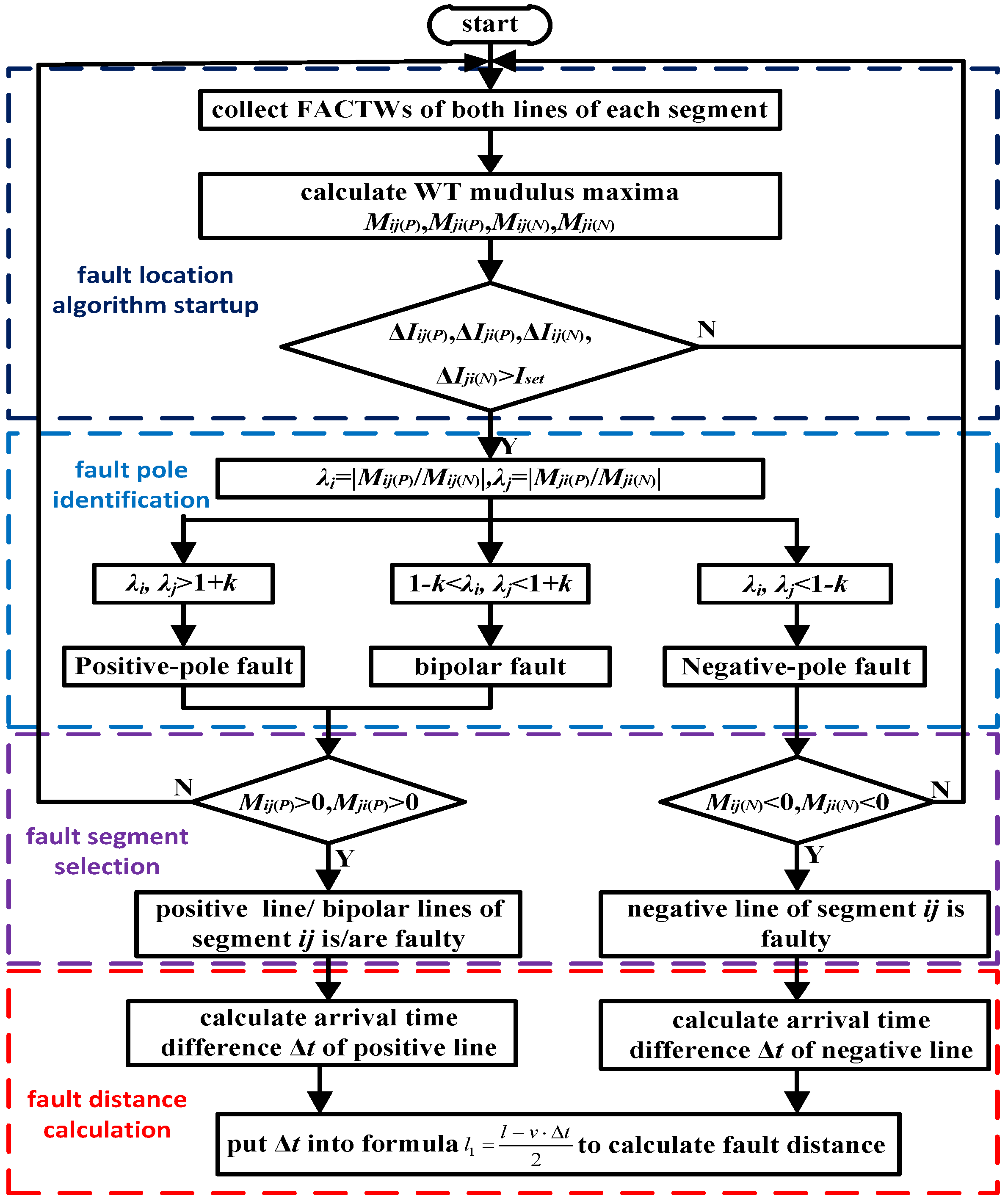
The flowchart of the fault-location scheme is illustrated in Figure 8. In practical applications, due to the current-limiting reactor and other primary-side equipment on both terminals of the DC line, the traveling wave signal will attenuate greatly. The amplitude of FACTW detected by the location device of the segment far from the fault point may be so small that the value of ΔI_i is less than I_set. In the case mentioned above, the segment would be considered as a non-fault segment.

4. Simulation and Analysis

4.1. Simulation Model

In order to verify the validity of the proposed fault-location scheme, a ±500 kV four-terminal MMC-HVDC power grid simulation model was built based on the design parameters of Chinese Zhangbei engineering project in PSCAD/EMTDC software (4.6.0.0, Manitoba HVDC Research Centre, Winnipeg, MB, Canada), whose schematic diagram is shown in Figure 9.

In Figure 9, D₁₂, D₂₁, D₁₃, D₃₁, D₂₄, D₄₂, D₃₄, D₄₃ are the fault-location devices installed at the terminals of each line to collect current traveling-wave signals. The detailed model of the MMCs and frequency-dependent model of the overhead lines are utilized. The R, L and C of the overhead line is 0.0114 Ω/km, 0.9542 mH/km, 0.01297 µF/km [22]. The lengths of each line are illustrated in Figure 8. Assume that the positive direction of current is from the DC bus to the DC line. The sampling frequency of the collected current signals is set to 1 MHz. The propagation velocity of traveling wave is 2.8425 × 10⁸ m/s, which is obtained from line parameters. In this paper, the “Haar” mother wavelet is chosen to detect the FACTW, because it provides the sharper edge. In addition, it is considered to be the simplest mother wavelet type available, which will demand less computational ability [19]. Besides, the scale of WT used in this paper is 3. The reliability coefficient k is set to be 0.5, if no special explanation in the following part.

4.2. Typical Fault Simulation

4.2.1. Metallic Single-Pole-Ground Fault

Without loss of generality, a metallic positive-pole-ground fault is set at f where is 68.1 km (equivalent to 30% of the total length of the segment L₁₂) from the Station I in the segment L₁₂. The fault-occurrence time is 0 ms. The waveforms of FACTWs of the positive lines in each segment detected by the fault-location devices and their WT modulus maxima are shown in Figure 10, Figure 11, Figure 12 and Figure 13. The simulation results of WT modulus maxima are shown in

Table 1. Simulation results of WT modulus maxima.

Segment Number	The First WT Modulus Maxima
	Mij(P)	Mji(P)	Mij(N)	Mji(N)
L12	0.4346	0.3541	−0.0928	−0.0860
L13	−0.4290	0.2608	0.0900	−0.0761
L24	−0.3466	0.2169	0.0823	−0.0667
L34	−0.2531	−0.2107	0.0739	0.0636

. The fault location results are indicated in

Table 2. Location results of monopolar fault.

Segment Number	λi	λj	Mij(P)	Mji(P)	Result
L12	4.68	4.12	>0	>0	Positive-pole-line fault
L13	4.77	3.43	<0	>0	Normal
L24	4.21	3.25	<0	>0	Normal
L34	3.42	3.31	<0	<0	Normal

.

As shown in Figure 10, Figure 11 and Figure 12, polarities of FACTWs at both terminals of the positive line in the segment L₁₂ detected by D₁₂ and D₂₁ are both positive. However, for the cases of segments L₁₃ and L₂₄, those detected by D₁₃ and D₃₁ are contrary to each other, and so are D₂₄ and D₄₂. Thus, the segment L₁₂ is judged as the faulted segment and the segments L₁₃ and L₂₄ are determined as the non-fault segments in light of the fault-segment identification criterion.

Since the total length of all the lines in the meshed network is 638 km, the two FACTWs will converge to the point where is 184.9 km from the Station III in the segment L₃₄. From Figure 13, polarities of FACTWs at both terminals of the positive line in the segment L₃₄ obtained by D₃₄ and D₄₃ are the same but both negative, the case of which is contrary to that of the faulted segment. Therefore, the segment L₃₄ is judged as the normal segment.

As shown in Figure 10, Figure 11, Figure 12 and Figure 13 and Table 2, since the ratios of both terminals in each segment are all much larger than 1.5, the positive pole is identified as the faulty pole and the data used for the following steps is taken from the fault-pole lines of each segment, which are the positive-pole lines in this simulation. Because the first WT modulus maxima at both terminals of the positive line in the segment L₁₂ are both larger than zero, the segment L₁₂ is judged as the faulted segment. Hence, the identification results of the faulty pole and the faulted segment are identical to the actual condition. Besides, the arrival time difference Δt is 0.32 ms as shown in Figure 10, and according to (14), the calculation result of fault distance calculation is 68.02 km, and the absolute error is 0.08 km, which is 0.04% of the total length of the segment L₁₂. Therefore, the fault-location algorithm has a high accuracy for single-pole-ground fault.

4.2.2. Bipolar Short-Circuit Fault

In this part, a bipolar short-circuit fault is set at f. The fault starting time is set as 0 ms and the fault resistance is 100 Ω. The simulation results of the first WT modulus maxima are shown in

Table 3. Simulation results of WT modulus maxima.

Segment Number	The First CWT Modulus Maxima
	Mij(P)	Mji(P)	Mij(N)	Mji(N)
L12	0.5630	0.4854	−0.5630	−0.4854
L13	−0.5522	0.3609	0.5522	−0.3609
L24	−0.4710	0.3511	0.4710	−0.3511
L34	−0.3518	−0.3393	0.3518	0.3393

. The fault location results are shown in

Table 4. Location results of bipolar fault.

Segment Number	λi	λj	Mij(P)	Mji(P)	Result
L12	1.00	1.00	>0	>0	Bipolar-line fault
L13	1.00	1.00	<0	>0	Normal
L24	1.00	1.00	<0	>0	Normal
L34	1.01	1.00	<0	<0	Normal

.

From the results of Table 4, the ratios of each segment are all very close to 1, so the fault type is identified as the bipolar short-circuit fault. As a result of the first WT modulus maxima at both ends of the positive line in the segment L₁₂ being both larger than zero, the segment L₁₂ is determined as the faulted segment. Thus, the fault is a bipolar short-circuit fault occurring on the segment L₁₂. Besides, since the arrival time difference Δt is 0.32 ms, the fault distance is calculated as 68.02 km, which is identical to the result of positive-pole-ground fault. In brief, different fault types cannot affect the accuracy of fault calculation.

4.3. Simulation for Influencing Factors

In this part, in order to investigate the factors that may affect the accuracy of the proposed fault-location scheme, extensive simulations were performed as follows.

4.3.1. Different Fault Resistances

Several negative-pole-ground faults with different fault resistances are set at f. The simulation results are shown in

Table 5. Simulation results of WT modulus maxima with different fault resistances.

Fault Resistance/Ω	Segment Number	The First Modulus Maxima
		Mij(P)	Mji(P)	Mij(N)	Mji(N)
0	L12	0.4346	0.3541	−0.0928	−0.0860
	L13	−0.4290	0.2608	0.0900	−0.0761
	L24	−0.3466	0.2169	0.0823	−0.0667
	L34	−0.2531	−0.2107	0.0739	0.0636
100	L12	0.2825	0.2302	−0.0603	−0.0559
	L13	−0.2788	0.1695	0.0585	−0.0495
	L24	−0.2253	0.1409	0.0535	−0.0434
	L34	−0.1645	−0.1370	0.0480	0.0414
300	L12	0.1521	0.1239	−0.0325	−0.0301
	L13	−0.1502	0.0913	0.0315	−0.0266
	L24	−0.1231	0.0759	0.0288	−0.0234
	L34	−0.0855	−0.0717	0.0259	0.0222

.

Table 5 shows that the absolute value of WT modulus maximum gradually decreases with the increase of fault resistance. Even so, as shown in

Table 6. Location results of fault with different fault resistances.

Fault Resistance/Ω	Faulty Pole	Faulted Segment	Calculation Result/km	Error/km
0	Negative	L12	68.02	0.08
100	Negative	L12	68.02	0.08
300	Negative	L12	68.02	0.08

, different fault resistances cannot affect the fault-pole identification, the fault-line selection, and the accuracy of the fault distance calculation, indicating that the fault location scheme has strong tolerance of fault resistance.

4.3.2. Different Fault Distances

In the segment L₁₂, without loss of generality, the metallic positive-pole-ground faults are set at different distances from the Station I. Fault-location results are shown in

Table 7. Location results of fault with different fault distances.

Fault Distance/km	Faulty Pole	Faulted Segment	Calculation Result/km	Error/km
22.7	Positive	L12	22.54	−0.16
45.4	Positive	L12	45.16	−0.12
68.1	Positive	L12	68.02	−0.08
90.8	Positive	L12	90.76	−0.04
113.5	Positive	L12	113.50	0.00
136.2	Positive	L12	136.24	0.04
158.9	Positive	L12	158.98	0.08
181.6	Positive	L12	181.72	0.12
204.3	Positive	L12	204.46	0.16

.

From the results in Table 7, it can be seen that the proposed fault-location scheme can accurately determine the exact fault position. As shown in Figure 14, the relative errors of fault distance calculation are all less than 0.1%, and are gradually reducing with the fault point moving from the both terminals to the midpoint of the line, and the error is zero when the fault occurs at the midpoint, which meets the requirements of the actual engineering.

From the above simulation results, the fault location scheme proposed in this paper is rarely influenced by fault type, fault resistance and fault distance, which have high reliability and accuracy.

5. Conclusions

In this paper, a traveling-wave-based fault-location scheme merely using the terminal measurements was proposed for MMC-MTDC grids. Considering the complex topology of MTDC systems, the scheme is divided into three stages, including faulty pole identification, faulty segment determination and fault-distance calculation. Referring to Zhangbei demonstration project in China, a ±500 kV four-terminal MMC-HVDC simulation model was constructed and extensive simulations were carried out. From the performed theoretical analysis and simulation results, the following conclusions could be drawn:

• The simulation results show that influencing factors, such as the fault type, fault resistance and fault distance, can hardly affect the correct operation of the proposed fault-location scheme.
• Only the FACTWs at different terminals are used in the proposed scheme, which eliminates the practical difficulty for identification of the subsequent surges.
• Despite the fault-location scheme being derived and simulated considering a MTDC grids with just a mesh, it can be applied easily and simply to MTDC grids with any number of meshes and can work properly.

References

1. Huang, L.; Yang, X.; Xu, P.; Zhang, F.; Ma, X.; Liu, T.; Hao, X.; Liu, W. The evolution and variation of sub-module topologies with DC-fault current clearing capability in MMC-HVDC. In Proceedings of the 2017 IEEE 3rd International Future Energy Electronics Conference and ECCE Asia (IFEEC 2017-ECCE Asia), Kaohsiung, Taiwan, 3–7 June 2017. [Google Scholar]
2. Nami, A.; Liang, J.; Dijkhuizen, F.; Demetriades, G.D. Modular Multilevel Converters for HVDC Applications: Review on Converter Cells and Functionalities. IEEE Trans. Power Electron. 2015, 30, 18–36. [Google Scholar] [CrossRef]
3. Li, X.; Yuan, Z.; Fu, J.; Wang, Y.; Liu, T.; Zhu, Z. Nanao multi-terminal VSC-HVDC project for integrating large-scale wind generation. In Proceedings of the 2014 IEEE PES General Meeting Conference & Exposition, National Harbor, MD, USA, 27–31 July 2014. [Google Scholar]
4. Tang, G.; He, Z.; Pang, H.; Huang, X.; Zhang, X.P. Basic topology and key devices of the five-terminal DC grid. CSEE J. Power Energy Syst. 2015, 1, 22–35. [Google Scholar] [CrossRef]
5. Sun, X.; Cao, S.; Bu, G.; Wang, H.; Lei, X.; Lu, B. Construction scheme of overhead line flexible HVDC grid. Power Syst. Technol. 2016, 40, 678–682. [Google Scholar] [CrossRef]
6. Tang, G.; Luo, X.; Wei, X. Multi-terminal HVDC and DC grid technology. Proc. CSEE 2013, 33, 8–17. [Google Scholar] [CrossRef]
7. Long, W.F.; Reeve, J.; McNichol, J.R.; Harrison, R.E.; Fletcher, D.E.; Bowles, J.P. Consideration for Implementing Multiterminal DC Systems. IEEE Trans. Power Appar. Syst. 1985, 104, 2521–2530. [Google Scholar] [CrossRef]
8. Das, S.; Santoso, S.; Gaikwad, A.; Patel, M. Impedance-based fault location in transmission networks: Theory and application. IEEE Access 2014, 2, 537–557. [Google Scholar] [CrossRef]
9. Dzienis, C.; Yelgin, Y.; Washer, M.; Maun, J.-C. Accurate impedance based fault location algorithm using communication between protective relays. In Proceedings of the 2015 Modern Electric Power Systems (MEPS), Wroclaw, Poland, 6–9 July 2015. [Google Scholar]
10. Bustamante-Mparsakis, X.; Maun, J.C.; Dzienis, C.; Jurisch, A. Travelling wave fault location based on pattern recognition. In Proceedings of the 2017 IEEE Manchester PowerTech, Manchester, UK, 18–22 June 2017. [Google Scholar]
11. Lopes, F.; Dantas, K.; Silva, K.; Costa, F.B. Accurate Two-Terminal Transmission Line Fault Location Using Traveling Waves. IEEE Trans. Power Deliv. 2017, PP, 1. [Google Scholar] [CrossRef]
12. Yuan, L.; Ning, K. Fault-location algorithms without utilizing line parameters based on the distributed parameter line model. IEEE Trans. Power Deliv. 2009, 24, 579–584. [Google Scholar] [CrossRef]
13. Song, G.; Cai, X.; Gao, S.; Suonan, J.; Li, G. Natural frequency based protection and fault location for VSC-HVDC transmission lines. In Proceedings of the 2011 International Conference on Advanced Power System Automation and Protection, Beijing, China, 16–20 October 2011. [Google Scholar]
14. He, Z.Y.; Liao, K.; Li, X.P.; Lin, S.; Yang, J.W.; Mai, R.K. Natural Frequency-Based Line Fault Location in HVDC Lines. IEEE Trans. Power Deliv. 2014, 29, 851–859. [Google Scholar] [CrossRef]
15. Xu, H.; Song, G. A novel traveling wave head identification method in VSC-HVDC based on parameter identification. In Proceedings of the 2015 5th International Conference on Electric Utility Deregulation and Restructuring and Power Technologies (DRPT), Changsha, China, 26–29 November 2015. [Google Scholar]
16. Chanda, N.K.; Fu, Y. ANN-based fault classification and location in MVDC shipboard power systems. In Proceedings of the 2011 North American Power Symposium, Boston, MA, USA, 4–6 August 2011. [Google Scholar]
17. Tang, L.; Ooi, B.T. Protection of VSC-multi-terminal HVDC against DC faults. In Proceedings of the 2002 IEEE 33rd Annual IEEE Power Electronics Specialists Conference (Cat. No.02CH37289), Cairns, Australia, 23–27 June 2002. [Google Scholar]
18. Shang, L.; Herold, G.; Jaeger, J.; Krebs, R.; Kumar, A. High-speed fault identification and protection in HVDC line using wavelet technique. In Proceedings of the 2001 IEEE Porto Power Tech Conference, Porto, Portugal, 10–13 September 2001. [Google Scholar]
19. Nanayakkara, O.K.; Rajapakse, A.D.; Wachal, R. Traveling-wave-based line fault location in star-connected multi-terminal HVDC systems. In Proceedings of the 2013 IEEE Power & Energy Society General Meeting, Vancouver, BC, Canada, 21–25 July 2013. [Google Scholar]
20. Kang, M.; Bo, Z. Based on the distribution network fault location simulation of wavelet modulus maxima. In Proceedings of the 2011 International Conference on Advanced Power System Automation and Protection, Beijing, China, 16–20 October 2011. [Google Scholar]
21. Song, S.; Zou, G. A Novel Busbar Protection Method Based on Polarity Comparison of Superimposed Current. IEEE Trans. Power Deliv. 2015, 30, 1914–1922. [Google Scholar] [CrossRef]
22. Vrana, T.K.; Yang, Y.; Jovcic, D.; Dennetiere, S.; Jardini, J.; Saad, H. The CIGRE B4 DC grid test system. Electra 2013, 270, 10–19. [Google Scholar]
Figure 1. A converter station with modular multilevel converter (MMC) configuration.
Energies 11 00401 g001
Figure 2. Two-terminal alternating current (AC) transmission system.
Energies 11 00401 g002
Figure 3. (a) Schematic of fault superimposed circuit and traveling wave propagation when internal fault f1 occurs; (b) Schematic of fault superimposed circuit and traveling wave propagation when external fault f2 occurs.
Energies 11 00401 g003
Figure 4. Fault superimposed circuit for the three-terminal MMC-based high voltage direct current (HVDC) grid.
Energies 11 00401 g004
Figure 5. Diagram of the line coupling effect.
Energies 11 00401 g005
Figure 6. Diagram of the bipolar short-circuit fault.
Energies 11 00401 g006
Figure 7. Schematic of traveling waves propagate in a two-terminal MMC-HVDC system.
Energies 11 00401 g007
Figure 8. Block diagram of the proposed fault location scheme.
Energies 11 00401 g008
Figure 9. Simulation model for the Zhangbei MMC-HVDC power grid.
Energies 11 00401 g009
Figure 10. (a) Waveforms of current traveling waves at both ends of the positive line in the segment L12; (b) Waveforms of their corresponding wavelet transform (WT) modulus maxima.
Energies 11 00401 g010
Figure 11. (a) Waveforms of current traveling waves at both ends of the positive line in the segment L24; (b) Waveforms of their corresponding WT modulus maxima.
Energies 11 00401 g011
Figure 12. (a) Waveforms of current traveling waves at both ends of the positive line in the segment L13; (b) Waveforms of their corresponding WT modulus maxima.
Energies 11 00401 g012
Figure 13. (a) Waveforms of current traveling waves at both ends of the positive line in the segment L34; (b) Waveforms of their corresponding WT modulus maxima.
Energies 11 00401 g013
Figure 14. Relative errors of fault distance calculation under different fault distances.
Energies 11 00401 g014