Robust Allocation of Reserve Policies for a Multiple-Cell Based Power System

 , , , and
Abstract
:1. Introduction
2. Methodology
2.1. Basic Power System Model
2.1.1. Constraints for Production Units
2.1.2. Constraints for Storage Units
2.2. Linear Decision Rule Based Robust Optimization of Reserve Allocation
2.3. One Cell-Based Reserve Allocation Model
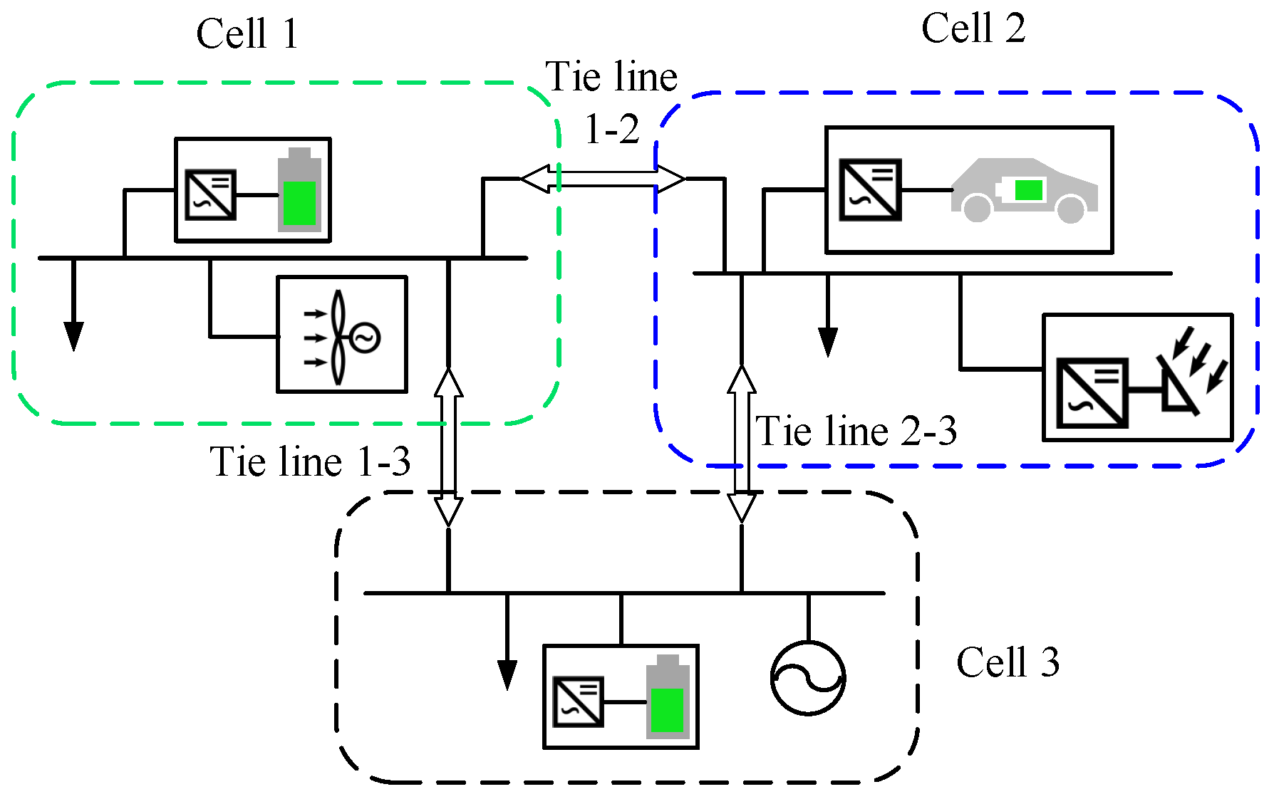
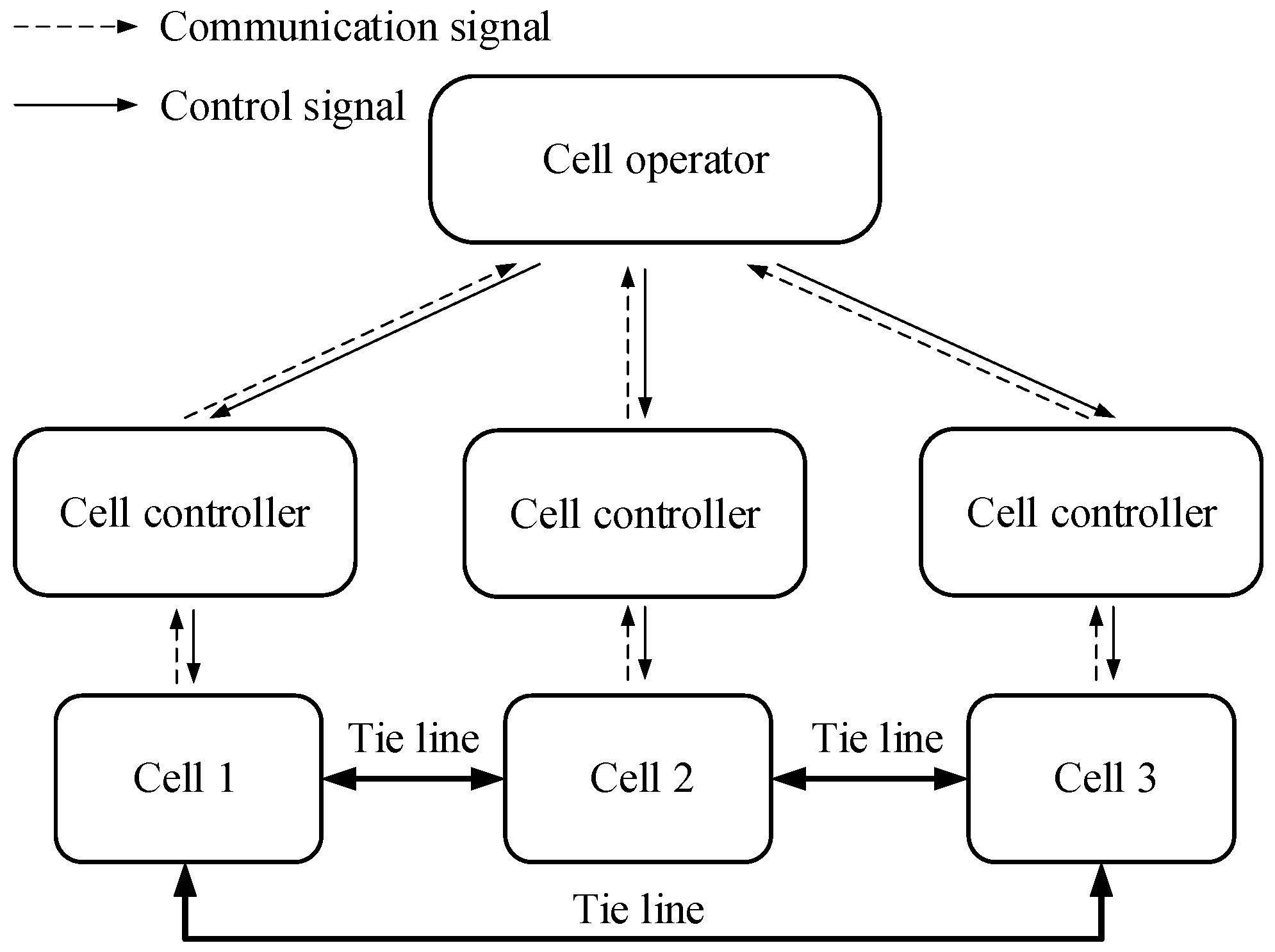
2.4. Multiple Cells-Based Reserve Allocation Model
3. Case Studies
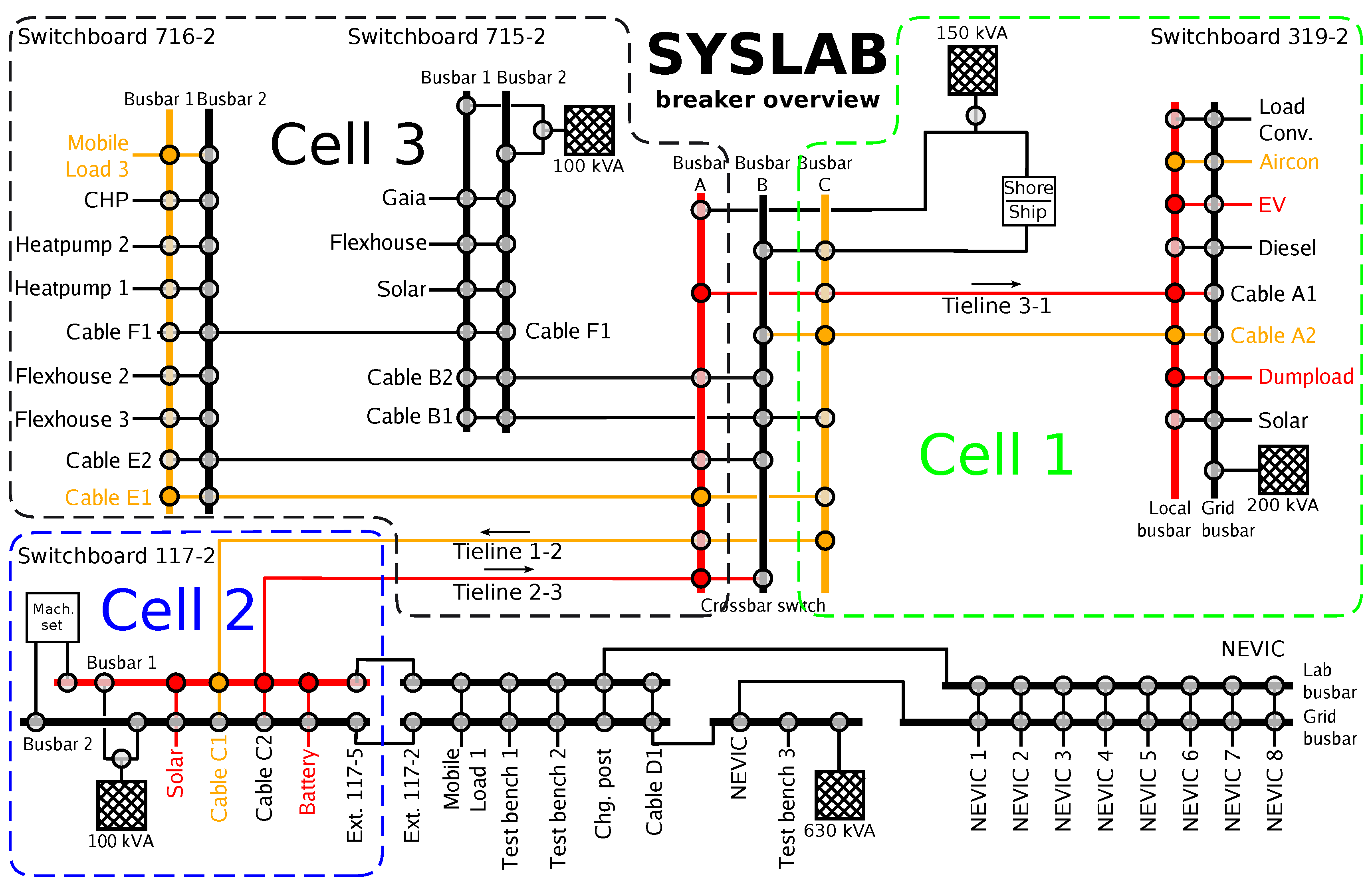
3.1. SYSLAB System
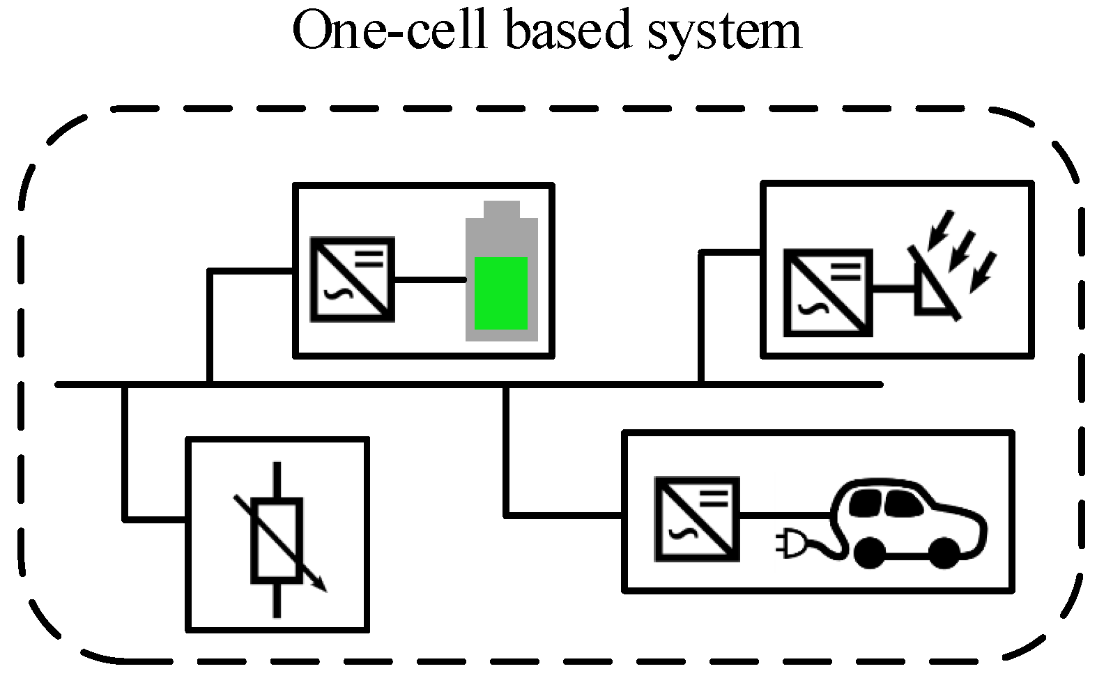
3.2. One Cell-Based Simulation
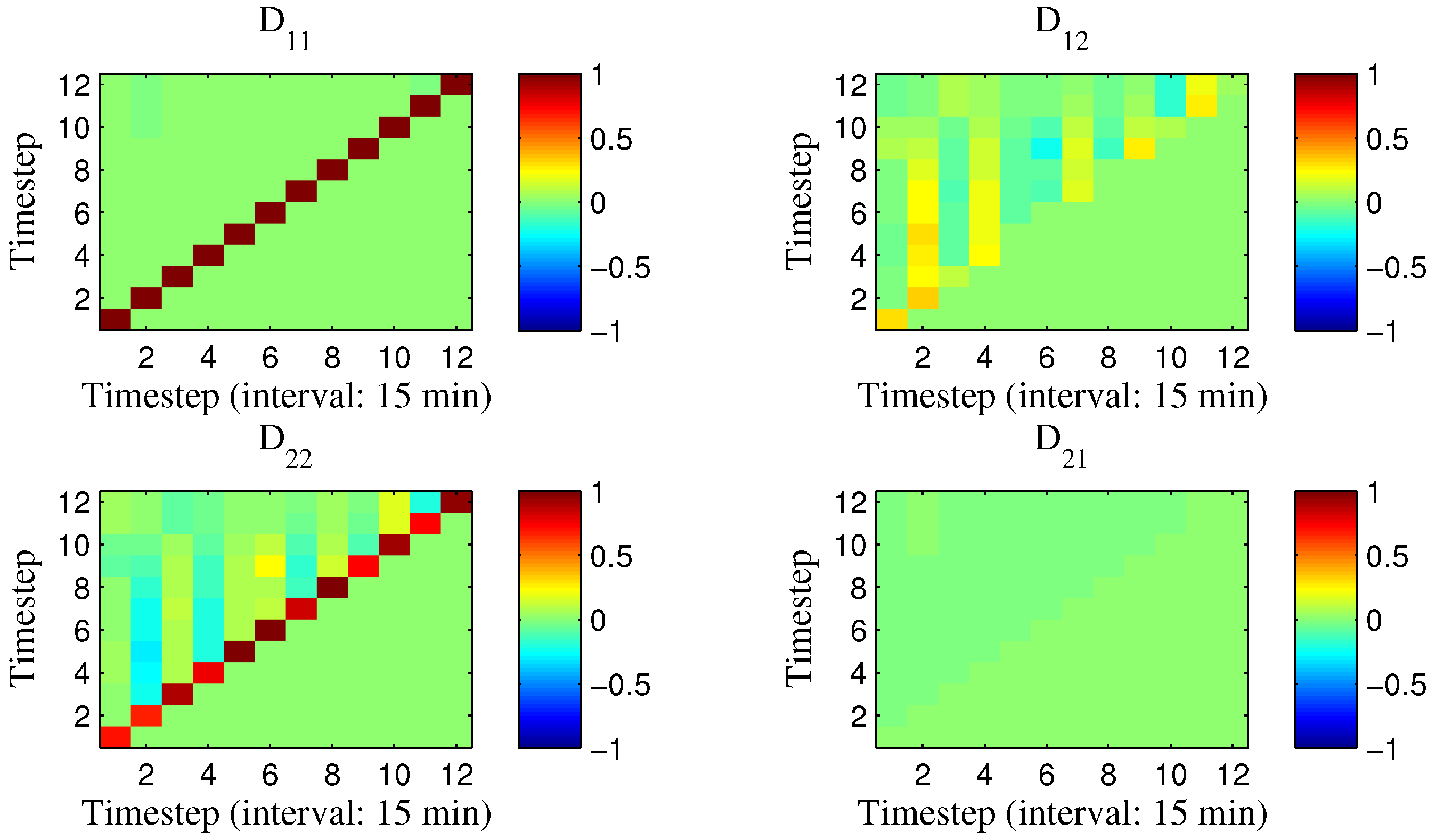
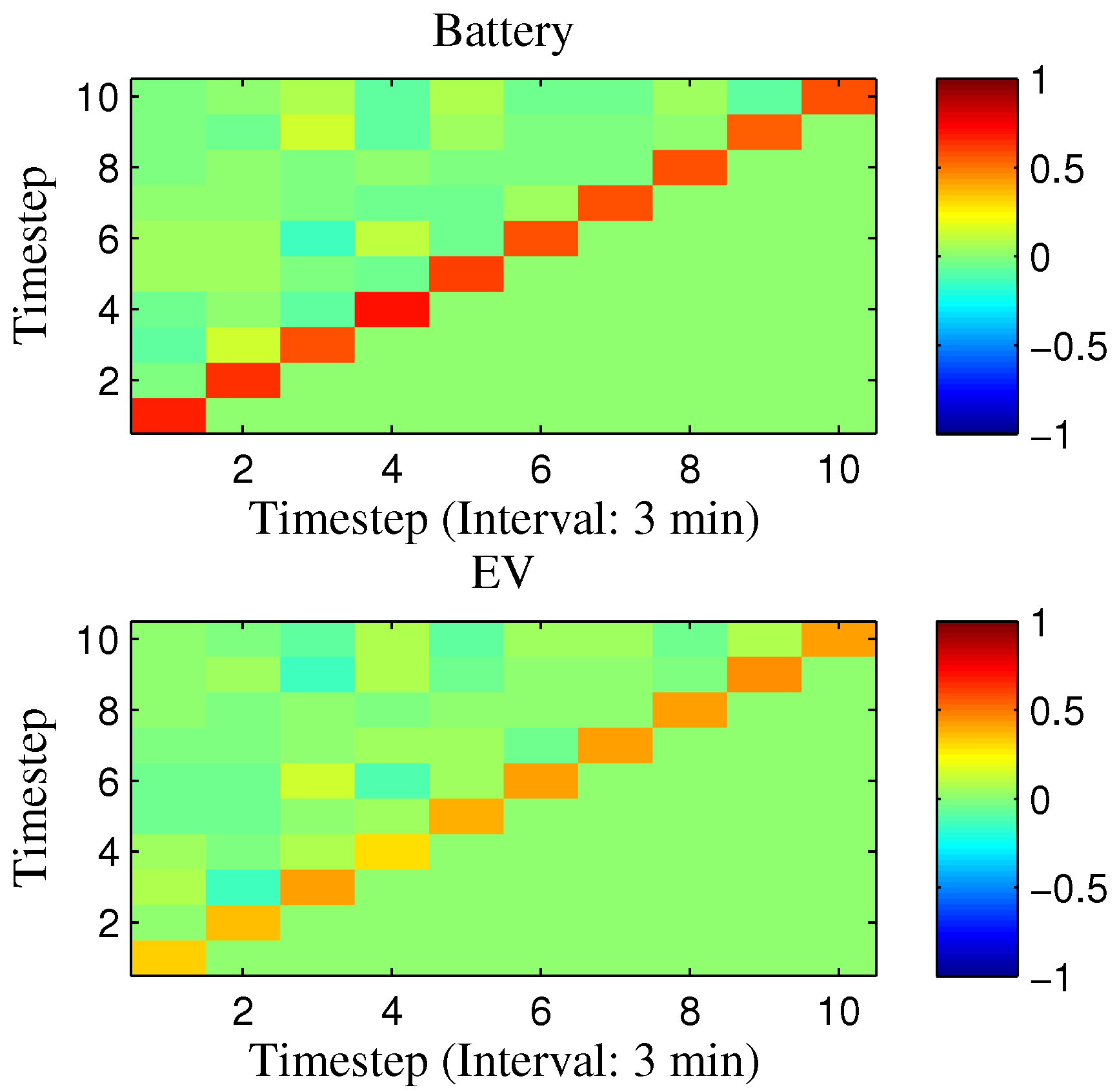
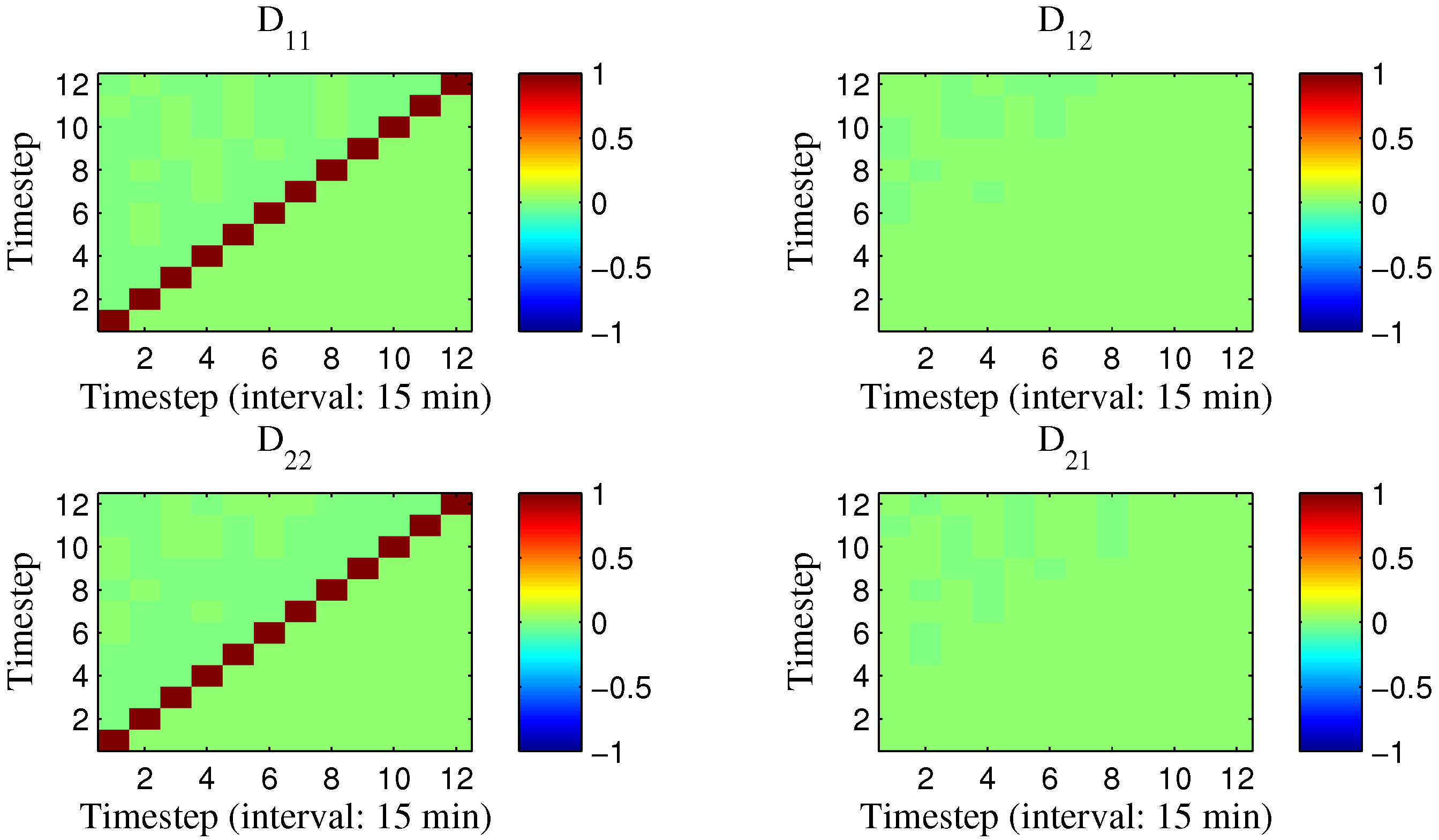
- Flexible-rate reserves [15]: is a diagonal matrix. This indicates the best possible response to uncertainty without time coupling. The previous uncertainty therefore has no impact on the present operation because the causality of the uncertainty is omitted. The optimization is over the elements of and the diagonal parts of .
- Policy-based reserves: Compared to the above scheme, this scheme considers the time coupling by taking as the lower-triangular form. It allows full exploitation of the information that will be available at each time step when the reserve is deployed.
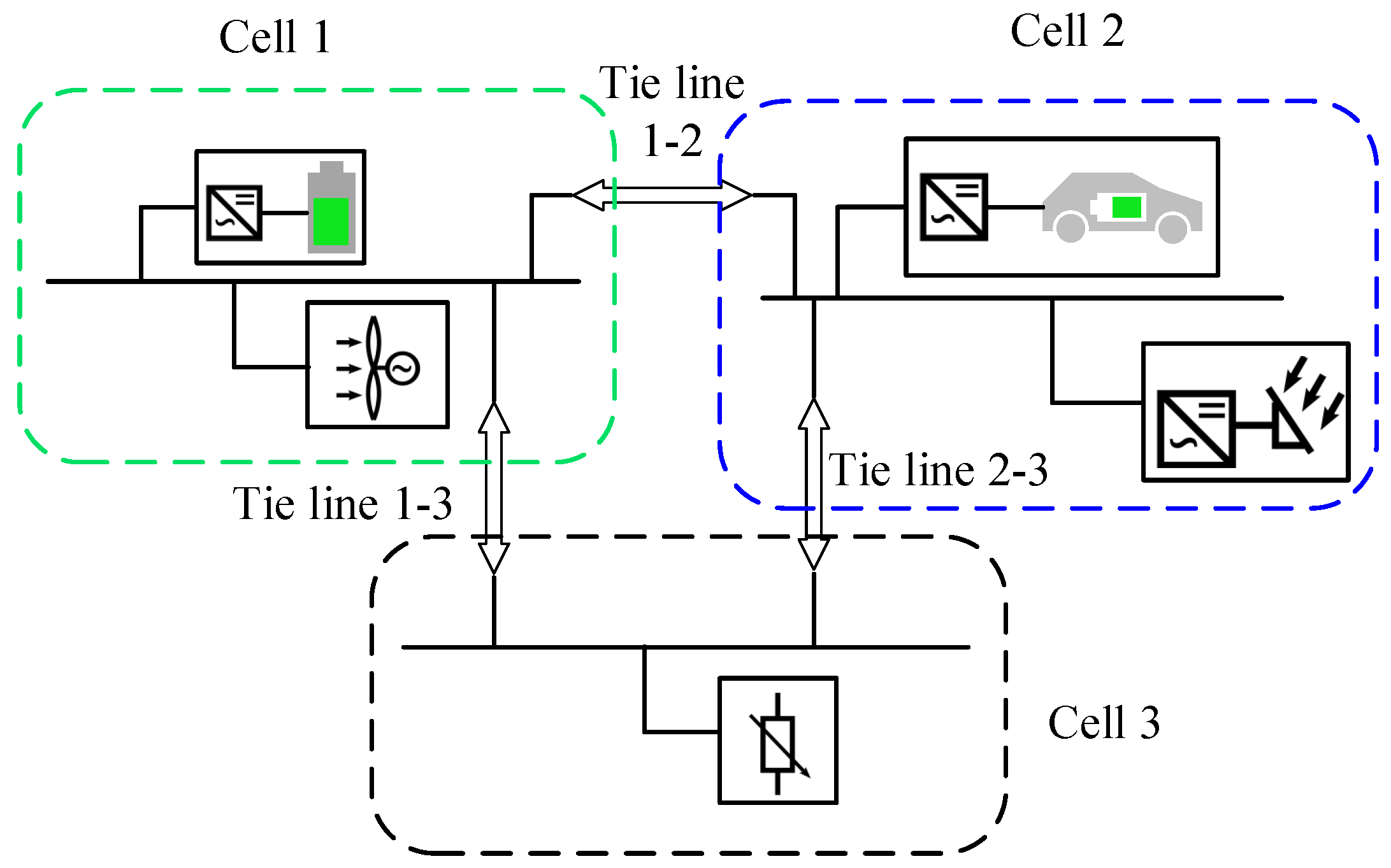
3.3. Three Cells-Based Simulation
3.3.1. Scenario 1
3.3.2. Scenario 2
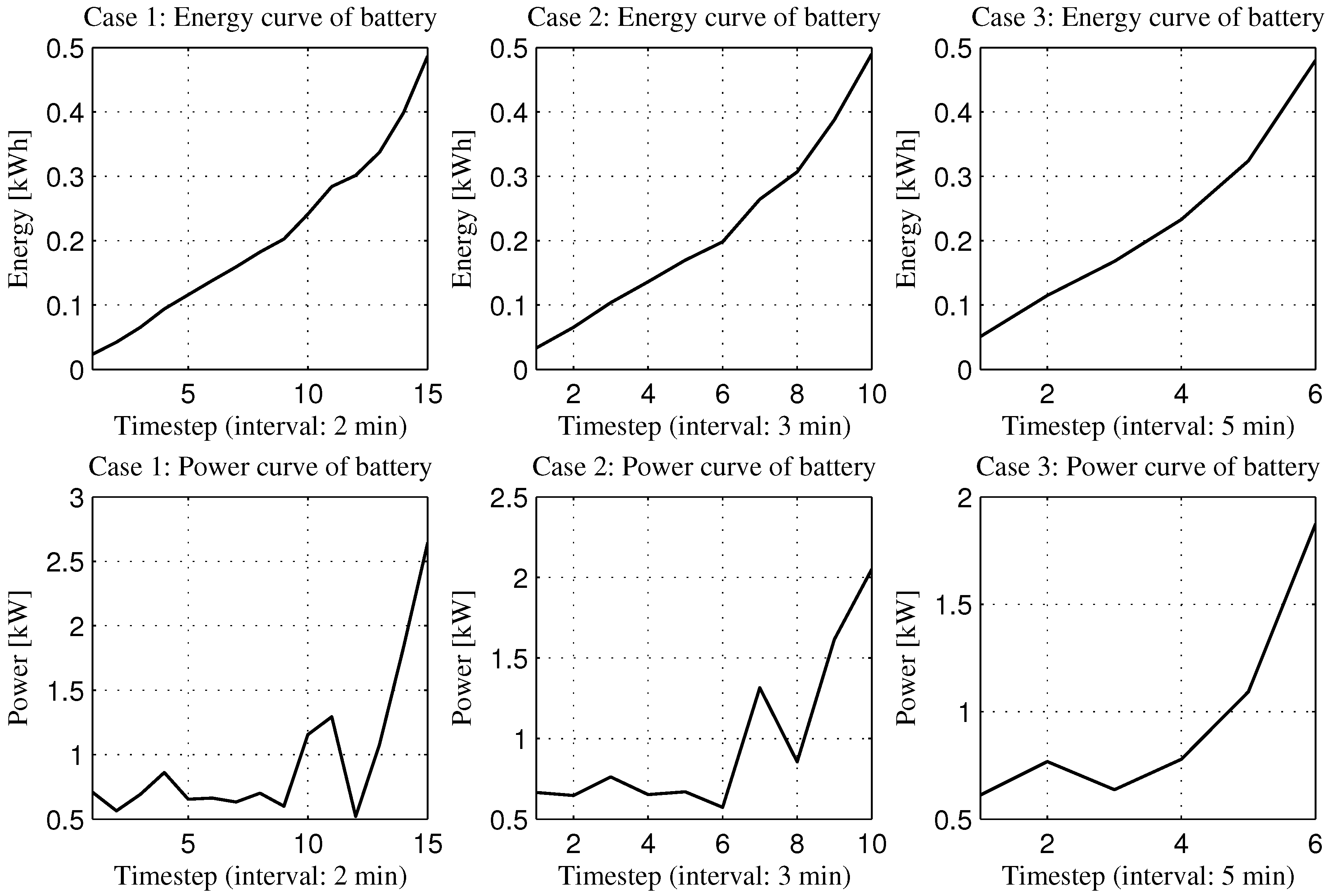
3.4. Impact of Time Interval
4. Discussion and Conclusions
Acknowledgments
Author Contributions
Conflicts of Interest
Nomenclature
Indices
| i | Index of inelastic participant. |
| j | Index of elastic participant. |
| l,m | Index of cell. |
Variable and Parameters
| Random forecast error vector. | |
| Participant j’s nominal elastic power. | |
| Nominal prediction of power injection or extraction of participant i. | |
| Stacked vector of participant j’s future control inputs. | |
| Stacked vector of participant j’s future states. | |
| Vector of participant j’s current states. | |
| Power injection or extraction of inelastic participant i. | |
| Stacked state transition matrix for participant j. | |
| Stacked state transition matrix for participant j. | |
| Stacked output matrix for participant j. | |
| Matrix adjusting power in response to . | |
| Map from uncertainty to inelastic power injection. | |
| T | Length of time horizon in steps. |
References
- Pineda, I.; Wilkes, J. Wind in Power: 2014, European Statistics; Technical Report; WindEurope: Brussels, Belgium, 2015; pp. 1–12. [Google Scholar]
- Agency, I.E. Renewable Energy Medium-Term Market Report 2015; Market Analysis and Forecasts to 2020; Technical Report; International Energy Agency: Paris, France, 2015. [Google Scholar]
- Dabra, V.; Paliwal, K.K.; Sharma, P.; Kumar, N. Optimization of photovoltaic power system: A comparative study. Prot. Control Mod. Power Syst. 2017, 2, 3. [Google Scholar] [CrossRef]
- Lan, T.; Strunz, K. Multiphysics Transients Modeling of Solid Oxide Fuel Cells: Methodology of Circuit Equivalents and Use in EMTP-Type Power System Simulation. IEEE Trans. Energy Convers. 2017, 32, 1309–1321. [Google Scholar] [CrossRef]
- Hu, J.; Yang, G.; Bindner, H.W.; Xue, Y. Application of Network-Constrained Transactive Control to Electric Vehicle Charging for Secure Grid Operation. IEEE Trans. Sustain. Energy 2017, 8, 505–515. [Google Scholar] [CrossRef]
- Hiskens, I.; Callaway, D. Achieving controllability of plug-in electric vehicles. In Proceedings of the 2009 IEEE Vehicle Power and Propulsion Conference (VPPC), Dearborn, MI, USA, 7–10 September 2009; IEEE: Piscataway, NJ, USA, 2009; pp. 1215–1220. [Google Scholar]
- Knezović, K.; Martinenas, S.; Andersen, P.B.; Zecchino, A.; Marinelli, M. Enhancing the Role of Electric Vehicles in the Power Grid: Field Validation of Multiple Ancillary Services. IEEE Trans. Transp. Electr. 2017, 3, 201–209. [Google Scholar] [CrossRef]
- De Martini, P.; Mani Chandy, K.; Fromer, N. Grid 2020 Towards a Policy of Renewable and Distributed Energy Resources; Technical Report; The Resnick Sustainability Institute at Caltech: Pasadena, CA, USA, 2012. [Google Scholar]
- Palizban, O.; Kauhaniemi, K.; Guerrero, J.M. Microgrids in active network management—Part I: Hierarchical control, energy storage, virtual power plants, and market participation. Renew. Sustain. Energy Rev. 2014, 36, 428–439. [Google Scholar] [CrossRef]
- Bessa, R.J.; Matos, M.A. Economic and technical management of an aggregation agent for electric vehicles: A literature survey. Eur. Trans. Electr. Power 2012, 22, 334–350. [Google Scholar] [CrossRef]
- ELECTRA IRP. European Liaison on Electricity Committed towards Research Activity Integrated Research Programm. Available online: http://www.electrairp.eu/ (accessed on 6 February 2018).
- Marinelli, M.; Pertl, M.; Rezkalla, M.M.; Kosmecki, M.; Canevese, S.; Obushevs, A.; Morch, A.Z. The Pan-European Reference Grid Developed in the ELECTRA Project for Deriving Innovative Observability Concepts in the Web-of-Cells Framework. In Proceedings of the 51st International Universities Power Engineering Conference (UPEC), Coimbra, Portugal, 6–9 September 2016; IEEE: Piscataway, NJ, USA, 2016. [Google Scholar]
- D’hulst, R.; Fernández, J.M.; Rikos, E.; Kolodziej, D.; Heussen, K.; Geibelk, D.; Temiz, A.; Caerts, C. Voltage and frequency control for future power systems: The ELECTRA IRP proposal. In Proceedings of the 2015 International Symposium on Smart Electric Distribution Systems and Technologies (EDST), Vienna, Austria, 8–11 September 2015; pp. 245–250. [Google Scholar]
- Morch, A.Z.; Jakobsen, S.H.; Visscher, K.; Marinelli, M. Future control architecture and emerging observability needs. In Proceedings of the 2015 IEEE 5th International Conference on Power Engineering, Energy and Electrical Drives (POWERENG), Riga, Latvia, 11–13 May 2015; pp. 234–238. [Google Scholar]
- Warrington, J.; Goulart, P.; Mariéthoz, S.; Morari, M. Policy-based reserves for power systems. IEEE Trans. Power Syst. 2013, 28, 4427–4437. [Google Scholar] [CrossRef]
- Jabr, R.A. Adjustable Robust OPF With Renewable Energy Sources. IEEE Trans. Power Syst. 2013, 28, 4742–4751. [Google Scholar] [CrossRef]
- Bertsimas, D.; Brown, D.B.; Caramanis, C. Theory and applications of robust optimization. SIAM Rev. 2011, 53, 464–501. [Google Scholar] [CrossRef]
- Hu, J.; Heussen, K.; Claessens, B.; Sun, L.; D’Hulst, R. Toward coordinated robust allocation of reserve policies for a cell-based power system. In Proceedings of the 2016 IEEE PES Innovative Smart Grid Technologies Conference Europe (ISGT-Europe), Ljubljana, Slovenia, 9–12 October 2016; pp. 1–6. [Google Scholar]
- Caerts, C.; Rikos, E.; Syed, M.; Guillo Sansano, E.; Merino-Fernández, J.; Rodriguez Seco, E.; Evenblij, B.; Rezkalla, M.M.N.; Kosmecki, M.; Temiz, A.; et al. Description of the Detailed Functional Architecture of the Frequency and Voltage Control Solution (Functional and Information Layer); Technical Report; Technical University of Denmark: Lyngby, Denmark, 2017. [Google Scholar]
- Stoft, S. Power System Economics: Designing Markets for Electricity, 1st ed.; Wiley-IEEE Press: New York, NY, USA, 2002. [Google Scholar]
- Brunner, H.; Tornelli, C.; Cabiati, M. The Web of Cells Control Architecture for Operating Future Power Systems; Technical Report; ELECTRA IRP—Public Deliverables: WP5 Increased Observability; European Union: Brussels, Belgium, 2018; under review. [Google Scholar]
- Lofberg, J.Y. YALMIP: A toolbox for modeling and optimization in MATLAB. In Proceedings of the International Symposium on Computer Aided Control Systems Design (CACSD), New Orleans, LA, USA, 2–4 September 2004; IEEE: Piscataway, NJ, USA, 2004; pp. 284–289. [Google Scholar]
- Optimization, Gurobi. Inc. Gurobi Optimizer Reference Manual; Technical Report; Gurobi Optimization, Inc.: Houston, TX, USA, 2017. [Google Scholar]
- Oliver, G.; Bindner, H. Building a test platform for agents in power system control: Experience from SYSLAB. In Proceedings of the International Conference on Intelligent Systems Applications to Power Systems (ISAP), Toki Messe, Niigata, Japan, 5–8 November 2007; IEEE: Piscataway, NJ, USA, 2007; pp. 1–5. [Google Scholar]
- Prostejovsky, A.M.; Marinelli, M.; Rezkalla, M.; Syed, M.H.; Guillo-Sansano, E. Tuningless Load Frequency Control Through Active Engagement of Distributed Resources. IEEE Trans. Power Syst. 2017. [Google Scholar] [CrossRef]
- Energinet. Ancillary Services to Be Delivered in Denmark Tender Conditions; Technical Report; Energinet: Erritsø, Denmark, 2017. [Google Scholar]


| Case | Simulation Duration | Time Interval | Horizon Length | Cost Index of Policy-Based Reserve | Cost Index of Flexible-Rate Reserve |
|---|---|---|---|---|---|
| 1 | 30 min | 2 min | 15 | 30.51 | 30.62 |
| 2 | 30 min | 3 min | 10 | 30.20 | 30.29 |
| 3 | 30 min | 5 min | 6 | 29.97 | 30.04 |
| Device | Test Case | (kW) | (kW) | (kW) | Description |
|---|---|---|---|---|---|
| Solar | 1, 3 Cell | 10.1 | 0.0 | 10.1 | Orientation |
| az. , el. | |||||
| Battery | 1, 3 Cell | 0.0 | −15.0 | 15 | Vanadium redox flow type |
| 190 kWh, initial state of charge is 50% | |||||
| EV | 1, 3 Cell | 0.0 | −2.0 | 2.0 | Bidirectional charger |
| 20 kWh, initial state of charge is 50% | |||||
| Mob. Load | 1, 3 Cell | −33.0 | −33.0 | 0.0 | Thyristor-contr. |
| Aircon | 3-Cell | 9.8 | 0.0 | 9.8 | Wind turbine |
© 2018 by the authors. Licensee MDPI, Basel, Switzerland. This article is an open access article distributed under the terms and conditions of the Creative Commons Attribution (CC BY) license (http://creativecommons.org/licenses/by/4.0/).
Share and Cite
Hu, J.; Lan, T.; Heussen, K.; Marinelli, M.; Prostejovsky, A.; Lei, X. Robust Allocation of Reserve Policies for a Multiple-Cell Based Power System. Energies 2018, 11, 381. https://doi.org/10.3390/en11020381
Hu J, Lan T, Heussen K, Marinelli M, Prostejovsky A, Lei X. Robust Allocation of Reserve Policies for a Multiple-Cell Based Power System. Energies. 2018; 11(2):381. https://doi.org/10.3390/en11020381
Chicago/Turabian StyleHu, Junjie, Tian Lan, Kai Heussen, Mattia Marinelli, Alexander Prostejovsky, and Xianzhang Lei. 2018. "Robust Allocation of Reserve Policies for a Multiple-Cell Based Power System" Energies 11, no. 2: 381. https://doi.org/10.3390/en11020381
APA StyleHu, J., Lan, T., Heussen, K., Marinelli, M., Prostejovsky, A., & Lei, X. (2018). Robust Allocation of Reserve Policies for a Multiple-Cell Based Power System. Energies, 11(2), 381. https://doi.org/10.3390/en11020381