Abstract
The thermal transmittance of building envelopes determines to a large extent the energy demand of buildings. Thus, there is a keen interest in having methods which can precisely evaluate thermal transmittance. From a scientific point of view, this study analyses the viability of the application of the thermometric method (THM), one of the most used methods in Spain. For this purpose, the test method has been improved by determining the adequate test conditions, the selection and installation of equipment, data acquisition and post-processing, and the estimation of uncertainty. We analyse eight case studies in a Mediterranean climate (Csa) to determine the potentials and limitations of the method. The results show that the values obtained through THM are valid under winter environmental conditions with relative uncertainties between 6% and 13%, while difficulties to perform the test in optimal conditions, and therefore to obtain valid results in warmer seasons, are detected. In this regard, the case studies which obtained a greater number of observations by performing the filtrate conditions were able to obtain representative results. Furthermore, there are significant differences depending on the kind of equipment and probes used during the experimental campaign. Finally, in warm climate regions a data filtrate can be considered for observations of a temperature difference higher than 5 °C, obtaining valid results for the case studies, although the rise in the thermal gradient can guarantee a greater stability of data.
1. Introduction
The concern about the environmental degradation of the planet has increased over the past few years. The building sector is among those most responsible for this phenomenon because of the amount of energy that it consumes [1].
In Europe, 24.79% of the total energy used in 2014 was attributed to residential buildings [2]. Likewise, the energy consumption has shown a tendency to increase 1% per year since 1990, so a higher energy consumption is expected [3]. In the case of the region of Andalusia (Spain), the residential building sector was responsible for 15.9% of the total energy consumption in 2016, which represents an increase of 4.1% in comparison with 2014 [4]. In this regard, it is important to highlight that the main source of consumption is attributed to meeting the heating demand [5,6,7].
Due to the fact that most of the energy consumed during the use phase of residential buildings comes from non-renewable resources, it is necessary to reduce the energy consumption in the existing building stock. Thus, the reduction of the energy demand and carbon dioxide emissions is the top priority objective of the building sector.
This improvement in energy behaviour must be made in existing buildings. Most of Spain’s building stock was built after the Spanish Civil War [8]. In this sense, as stated by Kurtz et al. [9], the thermal transmittance values of those buildings walls are higher than the limit values set by the Spanish Technical Building Code [10]. Furthermore, façades are the building envelope elements which most contribute to energy losses [11,12,13,14]. In this regard, Moyano Campos et al. [11] established that the analysed façades exceeded more of 100% the maximum acceptable value of the energy loss set by Spanish regulations, and that this situation could be solved by incorporating more insulation.
Thus, an improvement proposal regarding the thermal behaviour of external building walls represents one of the main performances in passive protection buildings [15]. Different procedures such as energy audits and checking the adequacy of safety and maintenance measures in buildings are fundamental to the study of building energy performances as well as to the proposal of energy conservation measures (ECMs) for building façades [16].
Thermal transmittance (also known as U-value) is one of the most significant properties which define the energy behaviour of a building envelope. The U-value is understood as the amount of heat which flows through a certain element per unit area and time.
This property can traditionally be determined by means of different procedures such as estimated methods [17] or in situ tests (the heat flow meter method) [18], or quantitative methods such as infrared thermography [19,20,21,22,23]). These methods have been widely studied in the literature and there are several studies in which the validity of their use is compared [24,25,26,27].
However, one of the most-used methods in Spain is called the thermometric method (THM) by the authors of this paper, and it is used by different trademarks. Most professionals use this method in order to perform energy audits. It can also be employed by authorised laboratories in the country [28,29]. However, there are no standards to develop the method, apart from specifications provided by the equipment’s manufacturers [30,31]. After a review of the literature, it was verified that there are no studies in which the viability of THM is analysed.
This method is characterised by the measurement of indoor and outdoor air temperatures as well as the internal surface temperature of the wall, but the heat flux is not measured. It is a method with simple theoretical and metrology fundamentals. These simplicities can lead to the fact that the obtained thermal transmittance value can be non-representative. In this context, Ficco et al. [25] indicated that in situ measurements with a simple theoretical development may face metrological problems, which can lead to atypical values with significant percentages of relative uncertainty.
However, THM shows a priori some advantages due to the fact that not using a heat flux plate allows the tests to be performed more easily and avoids the disturbance of the thermal behaviour of the wall caused by using the plate. According to this, Trethowen [32], Desogus et al. [33], and Cesaratto et al. [34] established that the presence of the heat flux plate could cause a disruption in the heat flux, consequently influencing the measurement result. Another important aspect to highlight is the reduction of the error achieved by avoiding the use of a heat flux plate. Peng and Wu [35] demonstrated that the main contribution to error in the thermal transmittance results is due to the heat flux measurement. Cucumo et al. [36] indicated that the location of the plate has an influence on the correct heat flux measurement. In this sense, Meng et al. [37] established that the maximum error of the U-value due to the use of thermocouples can be up to 6%, while that caused by the use of a heat flux plate can reach up to 26%.
Therefore, this research aimed to develop THM by establishing the best test conditions as well as the guidelines of the qualitative analysis of the wall, the installation of the equipment, data post-processing, and the estimation of uncertainty. The method is applied to eight study cases of heavy walls, and the results are compared to the estimated value of thermal transmittance according to ISO 6496 with the conductivity correction factors established by Pérez-Bella et al. [38] for the study areas.
2. Theory
THM is a development of the average method set in ISO 9869-1 [18]. It is based on the instantaneous measurement of the heat flow as well as the indoor and outdoor air temperatures under the conditions of a stationary regime:
where (W/m2) is the heat flux of the wall, (K) is the internal air temperature, and (K) is the external air temperature.
Using Newton’s Law of Cooling, the heat transfer per unit surface could be determined by the following expression:
where (W/(m2·K)) is the internal convective coefficient and (K) is the internal surface temperature of the wall.
From Equations (1) and (2), the equation used in THM is obtained:
It is important to highlight that this method always uses a fixed value of the internal convective coefficient, based on the value of the internal surface thermal resistance set in ISO 6946. Taking into account that the surface resistance is the reciprocal of the convective coefficient (Equation (4)) and the tabulated value of set by ISO 6946 for a vertical building envelope is 0.13 ((m2·K)/W), we obtain the equation of THM for the U-value measurement of façades (Equation (5)).
The fundamental difference between Equations (1) and (5) is in the numerator of the equations: in Equation (1) it is necessary to measure the heat flux of the wall, so the result is subject to a possible disruption of the heat flux due to the use of the plate [32,33,34] and has a high level of uncertainty associated with its location [35,36,37], while in Equation (5) the necessary variable measurement is only carried out by temperature probes, reducing the error associated with the probes’ location.
The temperature data are obtained by thermocouples, which measure both the exterior and interior environmental temperatures as well as the internal surface temperature of the wall [30,31].
Some manufacturers’ specifications in relation to the installation of the equipment and test durations are listed below [31]:
- Mounting the interior and exterior environmental temperature probes 30 cm away from the wall as well as at the same height as the internal surface temperature probes.
- No direct solar radiation.
- Measurements should be carried out during the night.
Moreover, it is advisable to have a significant difference between the internal and external temperatures, preferably higher than 15 °C.
Some of these specifications coincide with those set in ISO 9869-1. Requirements such as avoiding direct solar radiation on the façades and performing the test during the night are indicated in the standard, although the performance of the test during the night is established for light walls, while for heavy walls it should be longer.
However, these specifications are limited to ensure that the test is performed under correct metrological guidelines. Furthermore, the internal convective coefficient is utilised during the building design process to determine the energy behaviour, which overestimates the thermal transmittance [21,23], so the results obtained may not correspond to the actual values.
3. Quality Control, Data Post-Processing, and Uncertainty Quantification of the Method
Due to the fact that the metrological requirements given by the manufacturer do not address all factors that may affect the results of the test, we suggest some guidelines and criteria that should be applied when performing a THM test.
3.1. Test Conditions
In order to avoid direct solar radiation, the façade should preferably face north. Furthermore, the test should be conducted on walls without anomalies or pathologies, such as moisture or damage and defects.
Likewise, the manufacturers recommend a temperature difference higher than 15 °C [30,31]. In addition, the ideal test conditions will be those with no rainfall and a wind speed lower than 1 m/s. In this respect, the effects of these climatological variables can last from 2 to 6 h after these climate events disappear [23].
Before performing the test, it is advisable to evaluate the possible presence of non-homogeneities and thermal bridges in the wall through infrared thermography. This assessment should be carried out from both the internal and external sides of the wall by analysing them using ISO 6781 [39], as well as considering the following aspects:
- For at least 24 h before starting the test, the external air temperature must not vary more than ±10 °C from the existing temperature at the moment of starting the inspection.
- During the inspection, the outdoor air temperature must not vary more than ±5 °C and the indoor air temperature should vary no more than ±2 °C with respect to their initial values.
- Taking an infrared thermal image should be avoided in these three cases: when it is detected that the wall surface is not dry, if it is raining at the moment of performing the test, or if the wind speed is higher than 8 m/s.
3.2. Selecting and Installing the Equipment
In order to perform the test, a data logger and temperature probes are required. Moreover, it is advisable to mount a weather station near the wall in order to measure the external environmental conditions. Likewise, an IR camera is also required to apply ISO 6781.
Thermocouples should be as indicated by IEC 60584-1 [40]. There are different kinds of thermocouples, so we recommend a class-1 grade thermocouple due its tolerances and specifications. In terms of the data logger, it is also preferable to use programmable equipment which allow one to make data records with flexible periods from 1 s to 900 s.
Before performing the test, the equipment and probes should be correctly calibrated. Criteria for installing the equipment are as follows:
- Thermocouples measuring the internal surface temperature should be mounted with a space of 10 cm between them, as well as 20 mm away from the mortar joints of the pieces of brick of the internal side of the wall [31,37] at a height of 1.5 m above the floor [19]. The test described in ISO 6781 may be useful to determine the position of the mortar joints. According to the indications of Meng et al. [37], when the mortar joints cannot be determined, probes must be mounted without being vertically or horizontally aligned. A fixed mastic can also be used to achieve good contact with the wall [31]. In addition, it is important to avoid mounting the sensors in the corners, since the temperature is usually higher there than in the rest of the wall [23].
- Moreover, the internal and external air temperature sensors should be placed as horizontally aligned as possible, at a distance of 30 cm from the wall in order to avoid convective effects [31].
- In the case of those devices which directly measure air temperature, they should be placed at a distance of 30 cm from the internal side of the wall to prevent being affected by convective effects, with a height difference of 20 cm from the rest of the probes to avoid significant differences in temperature measurement.
- The weather station should be installed as near as possible to the wall under study, avoiding its installation towards other orientations.
3.3. Data Acquisition and Post-Processing
The test duration will depend on the typology of the wall to be analysed as well as the heat flow meter method: for light walls, the test should be carried out during the night to avoid direct solar radiation, while for heavy walls, it should last between 72 and 168 h [18]. The use of a data logger that records data for a period between 1 and 900 s will allow the variation of the frequency of data acquisition used in each test. By analysing the literature, the use of different sampling periods for the heat flow meter method and the quantitative methods of infrared thermography were detected: 2 min [41], 5 min [23,24,33], 15 min [19,25], 30 min [25], 60 min [25], or 90 min [25]. In this regard, we propose the use of sampling times of 15 min, which make the subsequent data analysis easier.
With respect to data post-processing, we recommend the use of a statistical programming language like R [42] due to its versatility when aggregating, validating, analysing, and reporting the obtained data. The generated dataset should be filtered by those observations with a high temperature gradient. This differential should be of 15 °C, although in those regions where the external environmental conditions make that requirement impossible, the use of a minor differential temperature should be considered. Likewise, only records obtained without precipitation and with a wind speed lower than 1 m/s should be considered.
The result obtained through the method is determined by the average value of the filtered subset of n values of thermal transmittance:
where (W/(m2·K)) is the U-value obtained from Equation (5) for a certain observation , and is the total number of filtered observations of the dataset.
To determine the validity of the U-value, the criterion proposed in ISO 9869-1 should be used. The valid results will be those with a difference less than 20% between the estimated value in ISO 6946 [17] and the value measured on site (see Equation (7)).
The estimated value is obtained from ISO 6946 as follows:
where (W/(m·K)) and (m) are the thermal conductivity and the thickness of each of the layers of the wall, respectively, and and ((m2·K)/W) are the internal and external surface resistances. These last two variables are obtained by means of the tabulated values in the standard ISO 6946.
One of the estimation method’s aspects which most affect the determination of the representative values is the existing difference between the used value of thermal conductivity and the actual value of each layer. This difference arises to the fact that in most existing databases, such as the constructive elements catalogue of the Spanish Technical Building Code in Spain [43], fixed environmental values are used in order to calculate the thermal properties according to ISO 10456 [44]. However, Pérez-Bella et al. [38] proposed the use of conductivity correction factors (CCF) for the conductivity values as a simplified procedure provided by ISO 10456 for all the Spanish cities, as it can be seen in the following expression:
where CCF (dimensionless) is the conductivity correction factor assigned to the municipality where the wall is located [38].
In order to determine the thickness of façade layers, a comparison with other buildings built during the same period as well as available design data and endoscopies can be used [18,25].
3.4. Estimating the Uncertainty
The uncertainty associated with THM is estimated by the combined standard uncertainty. The uncertainty contributions related to the measurement are due to the accuracy of the equipment employed (this accuracy is indicated in the manufacturers’ technical specifications) as well as the operative conditions associated with the performance of the test and the ambient conditions (see Table 1).

Table 1.
Uncertainty contributions estimated by the method.
Basing on the mathematical model of THM (Equation (5)), uncertainty contributions for the variables , , and are set. Due to the fact that (7.69) is a non-measured value, it has no contributions from uncertainty sources.
In order to estimate the combined standard uncertainty, ISO/IEC Guide 98-3:2008 [45] is used. According to this standard, the uncertainty for input quantities which are uncorrelated, as in the THM method, are determined by the following equation:
where are the sensitivity coefficients and are the uncertainty contributions.
As mentioned above, the sources of uncertainty are associated with three of the four variables, so there will be a total of three sensitivity coefficients. These sensitivity coefficients are partial derivatives from Equation (5) regarding the input variables , , and , which are used to describe how the output estimate changes according to the variations in these variables:
4. Experimental Campaign
In order to validate the method, eight walls from different building periods were monitored (see Figure 1). These façades are located in the city of Seville (case studies 1–6) and Cadiz (case studies 7–8) (see Table 2). They represent typical façade configurations found in these areas. In such cities, the climate is classified by Köppen and Geiger as Csa [46]: mild winters and hot summers.
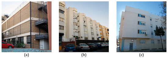
Figure 1.
Façades of some of the analysed buildings: (a) C-5 (1966), (b) C-6 (1981), and (c) C-7 (2004).
Table 2.
Technical characteristics and thermophysical properties of case studies 1–8.
The procedures described in Section 3 of this paper were applied to all walls (see Figure 2). The tests were conducted in winter (C-1, C-2, and C-3), summer (C-4, C-5, C-6, and C-7), and autumn (C-8). The duration of the tests was 72 h in all case studies and the equipment were configured with a sampling frequency of 15 min.
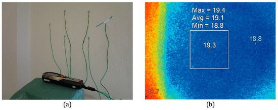
Figure 2.
(a) Installation of the equipment and (b) internal qualitative assessment by means of infrared thermography.
To carry out the tests, two data loggers with different probes were used (see Table 3) in order to determine possible existing deviations.
Table 3.
Main technical specifications of the employed equipment.
Design data of all case studies were obtained, so their compositions were determined by this source and the transmittance values were estimated by standard ISO 6946 (see Table 2).
5. Analysis and Results
The measured values during the experimental campaign for the different case studies can be seen in Figure 3. To show a simpler graphic, only the values measured by one of the data loggers are represented.
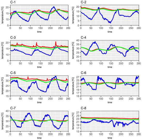
Figure 3.
Values of the temperature measured by the probes of data logger A: the internal air temperature (red), the internal surface temperature of the wall (green), and the external air temperature (blue).
Figure 4 represents the average values and the uncertainty estimations of the case studies obtained by means of THM. Furthermore, the estimated and obtained thermal transmittance values are reported in Table 4.
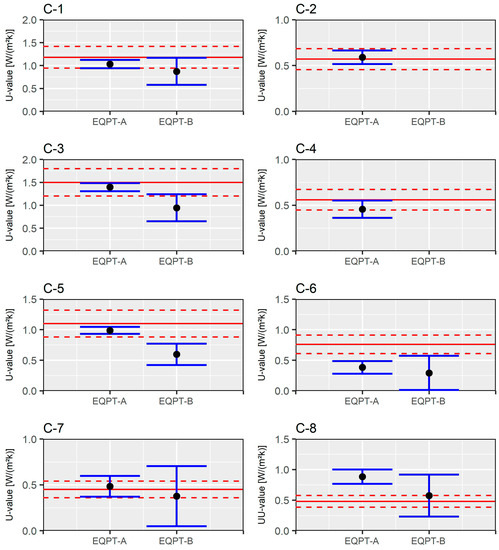
Figure 4.
Comparison of the thermal transmittance values obtained for the different case studies. EQPT-A denotes data logger A and EQPT-B indicates data logger B. The estimated value provided in ISO 6946 is represented by the red line [17] using the CCF of Pérez-Bella et al. [38], and the maximum acceptable difference (20%) regarding that value is represented by the dashed line.
Table 4.
Comparison of the obtained thermal transmittance values.
It is important to highlight the following aspects of the measured values:
- As can be observed, there were difficulties in the case studies (except in C-2 and C-5) to find observations with a difference higher than 10 °C between indoor and outdoor air temperatures. Also, in the case studies carried out during winter (C-1 and C-3), the largest temperature difference between the outdoor and the indoor air temperature was 7.2 °C, with values of the maximum temperature reaching up to 20.5 °C, which are records more commonly found in spring than in winter. For C-6 and C-8, there were few instances of a temperature difference registered higher than 5 °C.
- In most case studies, the value of the indoor air temperature was constant but with slight variations.
- In C-2 and C-4, the external temperature sensor of data logger B, connected by radio, stopped emitting a signal shortly after the beginning of the test, so data could not be obtained from this equipment.
- Regarding the difference between the measures recorded by both data loggers, meaningful variations in the measurement of the internal surface temperature were not detected, with average deviations of ±0.1 °C. However, there were significant differences between the indoor and outdoor air temperatures (see Figure 5).
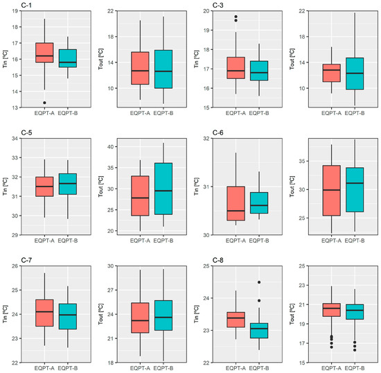 Figure 5. Box plots of the measurements of the indoor and outdoor air temperature recorded by both equipment setups. EQPT-A denotes data logger A and EQPT-B represents data logger B. The representation of case studies C-2 and C-4 is omitted due to the fact that the external probe was disconnected during the tests.
 - During the performance of the tests, no rainfall occurred and the wind speed was always lower than 1 m/s.
Due to the low thermal gradient registered during the measurements taken with mild outdoor air temperatures, we decided to filter the data for a differential temperature of 5 °C. The influence of using this post-processing on the obtained results is analysed in Figure 6 and Table 5.
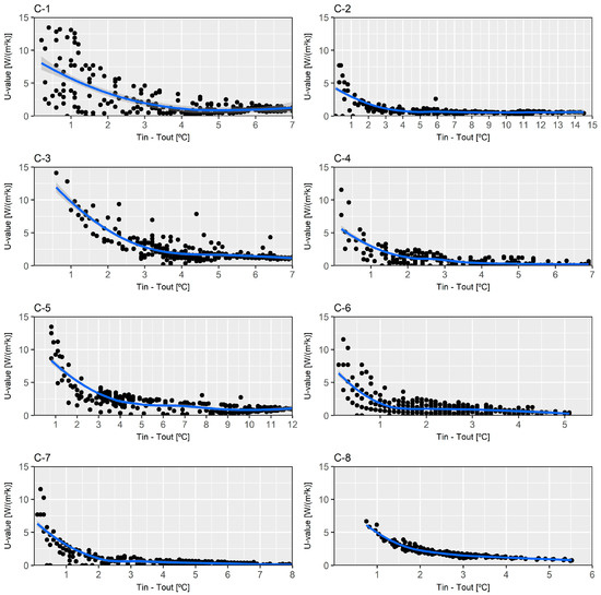
Figure 6.
Dispersion of U-value data according to the differences between the external and internal environmental temperatures. The local regression (LOESS) curve is represented by the blue line.
Table 5.
Comparison of the obtained values of thermal transmittance in C-2 and C-5 according to data management.
It can be seen by analysing the results that the values obtained in C-1, C-2, C-3, C-4, C-5, and C-7 were lower than 20% regarding the estimated value of thermal transmittance determined by means of the data obtained through data logger A. With respect to the uncertainty associated with these results, optimal values lower than 14% were obtained in C-1, C-2, C-3, and C-5. However, the values obtained were unacceptable (20–26%) in the rest of the walls. Thus, the method presented good behaviour in winter environmental conditions, whereas in summer, the results obtained in C-5 were valid due to the huge numbers of observations registered with differences higher than 5 °C. Nevertheless, the average results in C-6 and C-8 had meaningful differences regarding the estimated value of the façade due to the fact that a representative sample of data with a difference higher than 5 °C between the interior and exterior was not obtained, being lower than 3.46% and 5.19% of the total number of observations, respectively. Thus, in those case studies in which a percentage of filtered observations higher than 31.8% was acquired, the results obtained are representative. For this reason, it is very difficult to perform tests in optimal warm climate conditions, except in winter seasons.
On the other hand, the values obtained by data logger B only allowed us to obtain an average value inside the deviation of 20% regarding the estimated value of thermal transmittance for the case study C-7, but the high uncertainty associated with this result (86.5%) rendered it invalid. In the rest of the case studies, the average values obtained had differences higher than 20% regarding the estimated value, as well as inadmissible values of relative uncertainty.
Thus, differences between the results obtained by both data loggers with variations between 15.5% and 39.8% were detected.
This difference obtained between the two data loggers was not due to the possible presence of thermal discontinuities in the wall, since the façades were analysed before the installation of the probes. Likewise, all of the thermocouples used were put in the same location, according to the criteria established in Section 3 of this paper. In this sense, the variations presented by the measurements of indoor and outdoor air temperatures recorded by both sets of equipment (see Figure 5) were the main cause of the existing differences between their results, since the thermocouples for the internal surface temperature obtained records with average deviations of ±0.1 °C. This fact not only affected the thermal transmittance value obtained by Equation (5) for each observation, but also had an influence on the filtrate process, obtaining subsets with a different number of observations.
This circumstance was due to the fact that the indoor air temperature probe was located in the cable connection of the internal surface temperature probes in data logger B, so the measurement conditions of the indoor air temperature probe were different from those of the other equipment. Along this line, it is important to highlight that data logger B was placed very near to the internal air temperature probe of data logger A. Despite this, the data distributions showed significant variations between quartiles, with differences up to 1.1 °C. One of the reasons for this could be the fact that the equipment has to be put on a horizontal surface, so the measurement conditions were different from those of the probes of data logger A. Furthermore, the material of the horizontal surface on which data logger B was placed was not the same for all of the case studies, but varied according the elements available inside the rooms analysed.
With respect to the outdoor air temperature variable, the existing differences between both equipment setups were attributed to the technical characteristics of each probe. The difference in the data distribution of the thermohygrometer of data logger B was due to the lack of stability of the probe during the measurement regarding the probe of data logger A. Consequently, it was detected that the median of the external temperature data had variations higher than 0.5 °C as well as limit values up to 7.1 °C. Thus, the use of a class-1 grade K-type thermocouple to measure the variables necessary for THM could guarantee better stability in readings. Likewise, the use of equipment and probes that allow a considerable flexibility when installing them in the rooms of the walls to be analysed without being placed on a horizontal surface would reduce the differences of internal temperature data that were observed during the experimental campaign.
With respect to the need for processing the measured data, Figure 6 shows how differences higher than 5 °C between the internal and external ambient air allowed us to obtain representative values of thermal transmittance in most case studies for the measurements of data logger A. In this sense, the repeatability of the thermal transmittance values obtained in the different case studies was adequate, with variations between 11% and 35% regarding the obtained average value. However, the values obtained in C-2 and C-5 gave a greater stability in differences higher than 10 °C (see Table 5). In the case of data logger B the result did not vary, while for data logger A the obtained results reduced the associated uncertainty, and even values with a minor difference regarding the estimated value of the wall could be obtained.
This conclusion is in accordance with the recommendations established by several authors to perform other kinds of thermal transmittance tests, such as the heat flow meter method [25,33] and the quantitative methods of infrared thermography [19,23]. However, the use of filtered data for temperatures higher than 5 °C is an option to overcome the difficulties encountered by the performance of the tests in warm climate regions, as it is shown in the representative results obtained in the different case studies analysed during the experimental campaign.
6. Conclusions
In this paper, a detailed revision of one of the most-used methods to define the energy behaviour of a building envelope in Spain, the thermometric method (THM), is carried out. This method only has test recommendations given by the manufacturers of the equipment, but they are quite simple and do not guarantee the validity of the results. For this reason, we decided to provide the method with greater scientific rigour by establishing the operative conditions and optimal data management. In order to validate THM, the authors chose eight walls from different traditional façade typologies in the south of Spain.
Based on the results obtained in the experimental campaign of the eight case studies, we conclude the following:
- THM shows a more optimal behaviour in winter than in summer, with relative uncertainties between 6% and 13%.
- With respect to the environmental conditions in summer and autumn, despite obtaining average values with a difference lower than 20% regarding the estimated value of thermal transmittance, the associated uncertainty for the tests is unacceptable. Only in C-5 was an optimal value acquired, as temperature records with a difference higher than 10 °C were obtained.
- Differences in the average values as well as uncertainty according to the technical characteristics of the employed equipment were revealed. In this sense, the data logger which has probes with better features used for the tests obtained acceptable average results as well as adequate levels of uncertainty. However, the same cannot be said for the other equipment setup, because there were differences in the distribution of the measured temperature values.
- The typical characteristics of the Mediterranean climate (class Csa according to Köppen and Geiger’s climate classification) notably causes some difficulties in obtaining records with a temperature difference higher than 10 °C between the interior and exterior environments. In this regard, the results show that measurements with a high number of observations with a temperature difference higher than 5 °C were able to obtain representative results. Therefore, a thermal gradient of 5 °C can be considered for tests which are carried out in warm climate regions, although a higher difference would guarantee a decrease in the uncertainty and the achievement of more representative values.
To conclude, it is worth noting that there are few studies which analyse the use of a method in order to evaluate the U-value in warm climate typologies, such as the Mediterranean climate. It is also vital to highlight the lack of research studies in which THM is used. Our future work pertaining to this investigation will be the study of variations presented by the method regarding the use of internal convective coefficient values measured in situ, as well as the validation of its use in typologies of light walls.
Acknowledgments
The present study has been financed by “V Own Research Plan” University of Seville.
Author Contributions
All authors chose the case studies, performed the measurement, analysed the data, and wrote the paper together.
Conflicts of Interest
The authors declare no conflict of interest.
Nomenclature
| Tin | Internal air temperature (K) |
| Tout | External air temperature (K) |
| Ts,in | Internal surface temperature (K) |
| hin | Internal convective heat transfer coefficient (W/(m2·K)) |
| q | Heat flux (W/m2) |
| s | Thickness (m) |
| λ | Thermal conductivity (W/(m·K)) |
| R | Thermal resistance ((m2·K)/W) |
| Rs,in | Internal surface thermal resistance ((m2·K)/W) |
| Rs,out | External surface thermal resistance ((m2·K)/W) |
| U | Thermal transmittance (W/(m2·K)) |
| CCF | Conductivity correction factor (dimensionless) |
References
- Pérez-Lombard, L.; Ortiz, J.; Pout, C. A review on buildings energy consumption information. Energy Build. 2008, 40, 394–398. [Google Scholar] [CrossRef]
- European Environment Agency. Final Energy Consumption by Sector and Fuel (2017); European Environment Agency: Copenhagen, Denmark, 2017. [Google Scholar]
- European Academy of Bolzano. European Project iNSPiRe Report; European Academy of Bolzano: Bolzano, Italy, 2015. [Google Scholar]
- Andalusian Energy Agency. Energy Data of Andalusia; Andalusian Energy Agency: Seville, Spain, 2015.
- Ecology and Development Foundation (ECODES). Archive ECODES. City and Building: Environmental Impacts; Ecology and Development Foundation: Bend, Oregon, 2009. [Google Scholar]
- Institute for the Energy Diversification and Saving. Balance of the Final Energy Consumption in Year 2015; Institute for the Energy Diversification and Saving: Seville, Spain, 2016. (In Spain) [Google Scholar]
- Sánchez-García, D.; Sánchez-Guevara, C.; Rubio-Bellido, C. The adaptive approach to thermal comfort in Seville. An. Edif. 2016, 2, 38–48. [Google Scholar] [CrossRef]
- Gangolells, M.; Casals, M.; Forcada, N.; MacArulla, M.; Cuerva, E. Energy mapping of existing building stock in Spain. J. Clean. Prod. 2016, 112, 3895–3904. [Google Scholar] [CrossRef]
- Kurtz, F.; Monzón, M.; López-Mesa, B. Energy and acoustics related obsolescence of social housing of Spain’s post-war in less favoured urban areas. The case of Zaragoza. Inf. Constr. 2015, 67, m021. [Google Scholar] [CrossRef]
- The Government of Spain. Royal Decree 314/2006. Approving the Spanish Technical Building Code CTE-DB-HE-1; The Government of Spain: Madrid, Spain, 2013.
- Moyano Campos, J.J.; Antón García, D.; Rico Delgado, F.; Marín García, D. Threshold Values for Energy Loss in Building Façades Using Infrared Thermography. In Sustainable Development and Renovation in Architecture, Urbanism and Engineering; Springer International Publishing: Basel, Switzerland, 2017; pp. 427–437. [Google Scholar]
- Mortarotti, G.; Morganti, M.; Cecere, C. Thermal analysis and energy-efficient solutions to preserve listed building façades: The INA-Casa building heritage. Buildings 2017, 7, 56. [Google Scholar] [CrossRef]
- Park, K.; Kim, M. Energy Demand Reduction in the Residential Building Sector: A Case Study of Korea. Energies 2017, 10, 1506. [Google Scholar] [CrossRef]
- Battista, G.; Evangelisti, L.; Guattari, C.; Basilicata, C.; de Lieto Vollaro, R. Buildings Energy Efficiency: Interventions Analysis under a Smart Cities Approach. Sustainability 2014, 6, 4694–4705. [Google Scholar] [CrossRef]
- Suárez, R.; Fragoso, J. Passive strategies for energy optimisation of social housing in the Mediterranean climate. Inf. Constr. 2016, 68, e136. [Google Scholar] [CrossRef]
- Serrano Lanzarote, B.; Sanchis Cuesta, A. The Technical Inspection of Buildings as an instrument for the energy improvement of existing buildings. Inf. Constr. 2015, 67, nt003. [Google Scholar] [CrossRef]
- International Organization for Standardization. ISO 6946:2007—Building Components and Building Elements—Thermal Resistance and Thermal Transmittance—Calculation Method; International Organization for Standardization: Geneva, Switzerland, 2007. [Google Scholar]
- International Organization for Standardization. ISO 9869-1:2014—Thermal Insulation—Building Elements—In Situ Measurement of Thermal Resistance and Thermal Transmittance. Part 1: Heat Flow Meter Method; International Organization for Standardization: Geneva, Switzerland, 2014. [Google Scholar]
- Albatici, R.; Tonelli, A.M. Infrared thermovision technique for the assessment of thermal transmittance value of opaque building elements on site. Energy Build. 2010, 42, 2177–2183. [Google Scholar] [CrossRef]
- Madding, R. Finding R-values of stud-frame constructed houses with IR thermography. Proc. InfraMation 2008, 2008, 261–277. [Google Scholar]
- Dall’O, G.; Sarto, L.; Panza, A. Infrared screening of residential buildings for energy audit purposes: Results of a field test. Energies 2013, 6, 3859–3878. [Google Scholar] [CrossRef]
- Fokaides, P.A.; Kalogirou, S.A. Application of infrared thermography for the determination of the overall heat transfer coefficient (U-Value) in building envelopes. Appl. Energy 2011, 88, 4358–4365. [Google Scholar] [CrossRef]
- Tejedor, B.; Casals, M.; Gangolells, M.; Roca, X. Quantitative internal infrared thermography for determining in-situ thermal behaviour of façades. Energy Build. 2017, 151, 187–197. [Google Scholar] [CrossRef]
- Evangelisti, L.; Guattari, C.; Gori, P.; De Lieto Vollaro, R. In situ thermal transmittance measurements for investigating differences between wall models and actual building performance. Sustainability 2015, 7, 10388–10398. [Google Scholar] [CrossRef]
- Ficco, G.; Iannetta, F.; Ianniello, E.; D’Ambrosio Alfano, F.R.; Dell’Isola, M. U-value in situ measurement for energy diagnosis of existing buildings. Energy Build. 2015, 104, 108–121. [Google Scholar] [CrossRef]
- Choi, D.S.; Ko, M.J. Comparison of Various Analysis Methods Based on Heat Flowmeters and Infrared Thermography Measurements for the Evaluation of the In Situ Thermal Transmittance of Opaque Exterior Walls. Energies 2017, 10, 1019. [Google Scholar] [CrossRef]
- Nardi, I.; Paoletti, D.; Ambrosini, D.; De Rubeis, T.; Sfarra, S. U-value assessment by infrared thermography: A comparison of different calculation methods in a Guarded Hot Box. Energy Build. 2016, 122, 211–221. [Google Scholar] [CrossRef]
- Regional Government of Andalusia. Catalog of Services Offered by Quality Control Laboratories of the Regional Government of Andalusia—January 2017; Regional Government of Andalusia: Sevilla, Spain, 2017.
- The Government of Spain. 5th Registry, Entities and Quality Control Laboratories of Building; Ther Government of Spain: Madrid, Spain, 2017.
- KIMO Instruments. Determination of U Coefficient; KIMO Instruments: Montpon-Menesterol, France, 2010. [Google Scholar]
- Testo AG. U-Value Measurement; Testo AG: Lenzkirch, Germany, 2014. [Google Scholar]
- Trethowen, H. Measurement errors with surface-mounted heat flux sensors. Build. Environ. 1986, 21, 41–56. [Google Scholar] [CrossRef]
- Desogus, G.; Mura, S.; Ricciu, R. Comparing different approaches to in situ measurement of building components thermal resistance. Energy Build. 2011, 43, 2613–2620. [Google Scholar] [CrossRef]
- Cesaratto, P.G.; De Carli, M.; Marinetti, S. Effect of different parameters on the in situ thermal conductance evaluation. Energy Build. 2011, 43, 1792–1801. [Google Scholar] [CrossRef]
- Peng, C.; Wu, Z. In situ measuring and evaluating the thermal resistance of building construction. Energy Build. 2008, 40, 2076–2082. [Google Scholar] [CrossRef]
- Cucumo, M.; De Rosa, A.; Ferraro, V.; Kaliakatsos, D.; Marinelli, V. A method for the experimental evaluation in situ of the wall conductance. Energy Build. 2006, 38, 238–244. [Google Scholar] [CrossRef]
- Meng, X.; Yan, B.; Gao, Y.; Wang, J.; Zhang, W.; Long, E. Factors affecting the in situ measurement accuracy of the wall heat transfer coefficient using the heat flow meter method. Energy Build. 2015, 86, 754–765. [Google Scholar] [CrossRef]
- Pérez-Bella, J.M.; Domínguez-Hernández, J.; Cano-Suñén, E.; Del Coz-Díaz, J.J.; Álvarez Rabanal, F.P. A correction factor to approximate the design thermal conductivity of building materials. Application to Spanish façades. Energy Build. 2015, 88, 153–164. [Google Scholar] [CrossRef]
- International Organization for Standardization. ISO 6781:1983—Thermal Insulation—Qualitative Detection of Thermal Irregularities in Building Envelopes—Infrared Method; International Organization for Standardization: Geneva, Switzerland, 1983. [Google Scholar]
- International Electrotechnical Commission. IEC 60584-1:2013—Thermocouples—Part 1: EMF Specifications and Tolerances; International Electrotechnical Commission: Geneva, Switzerland, 2013. [Google Scholar]
- Meng, X.; Gao, Y.; Wang, Y.; Yan, B.; Zhang, W.; Long, E. Feasibility experiment on the simple hot box-heat flow meter method and the optimization based on simulation reproduction. Appl. Therm. Eng. 2015, 83, 48–56. [Google Scholar] [CrossRef]
- Ihaka, R.; Gentleman, R. R: A Language for Data Analysis and Graphics. J. Comput. Graph. Stat. 1996, 5, 299–314. [Google Scholar]
- Eduardo Torroja Institute for Construction Science. Constructive Elements Catalogue of the CTE; Eduardo Torroja Institute for Construction Science: Madrid, Spain, 2010. [Google Scholar]
- International Organization for Standardization. ISO 10456:2007—Building Materials and Products—Hygrothermal Properties—Tabulated Design Values and Procedures for Determining Declared and Design Thermal Values; International Organization for Standardization: Geneva, Switzerland, 2007. [Google Scholar]
- International Organization for Standardization. ISO/IEC Guide 98-3:2008—Uncertainty of Measurement—Part 3: Guide to the Expression of Uncertainty in Measurement (GUM:1995); International Organization for Standardization: Geneva, Switzerland, 2008. [Google Scholar]
- Rubel, F.; Kottek, M. Observed and projected climate shifts 1901–2100 depicted by world maps of the Köppen-Geiger climate classification. Meteorol. Z. 2010, 19, 135–141. [Google Scholar] [CrossRef]


© 2018 by the authors. Licensee MDPI, Basel, Switzerland. This article is an open access article distributed under the terms and conditions of the Creative Commons Attribution (CC BY) license (http://creativecommons.org/licenses/by/4.0/).