Solving the Energy Efficient Coverage Problem in Wireless Sensor Networks: A Distributed Genetic Algorithm Approach with Hierarchical Fitness Evaluation


Abstract

1. Introduction
2. Energy Efficient Coverage Problem in WSN
2.1. Problem Formulation
2.2. Related Work
3. Methodology: DGA for the EEC Problem
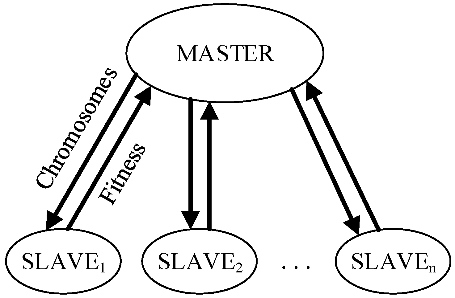
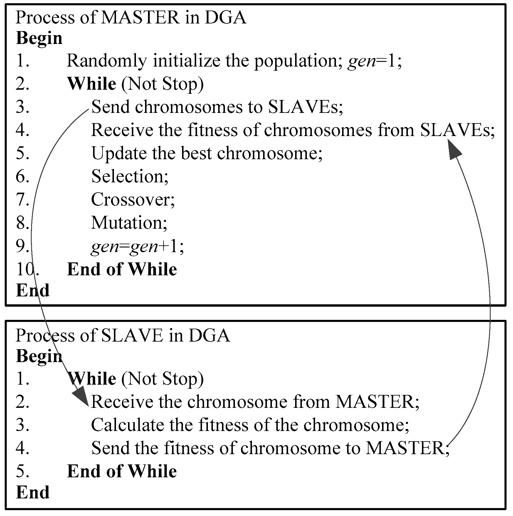
3.1. Distributed Framework of DGA
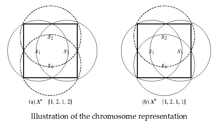
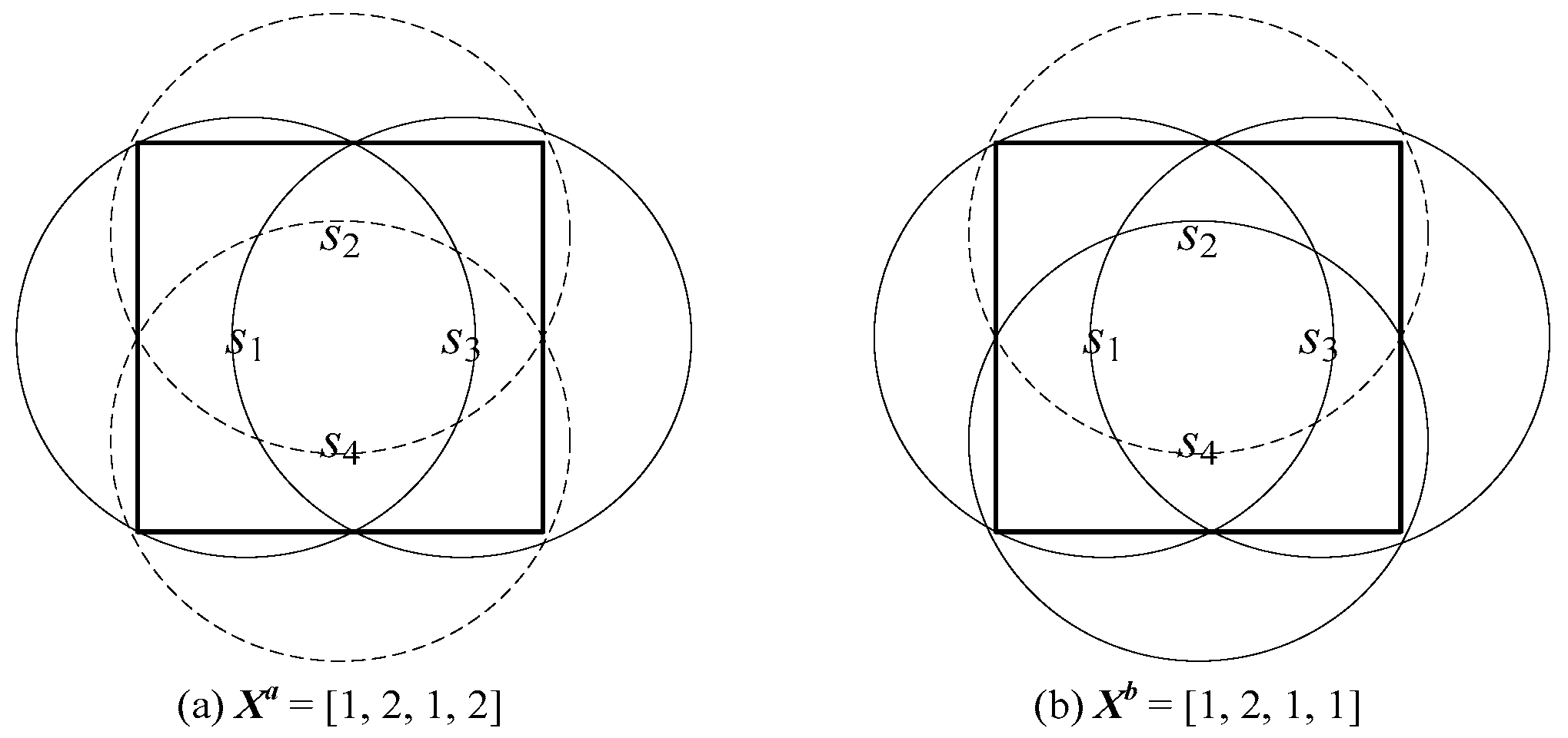
3.2. Chromosome Representation
3.3. Hierarchical Fitness Evaluation
3.4. Genetic Operators
3.4.1. Selection
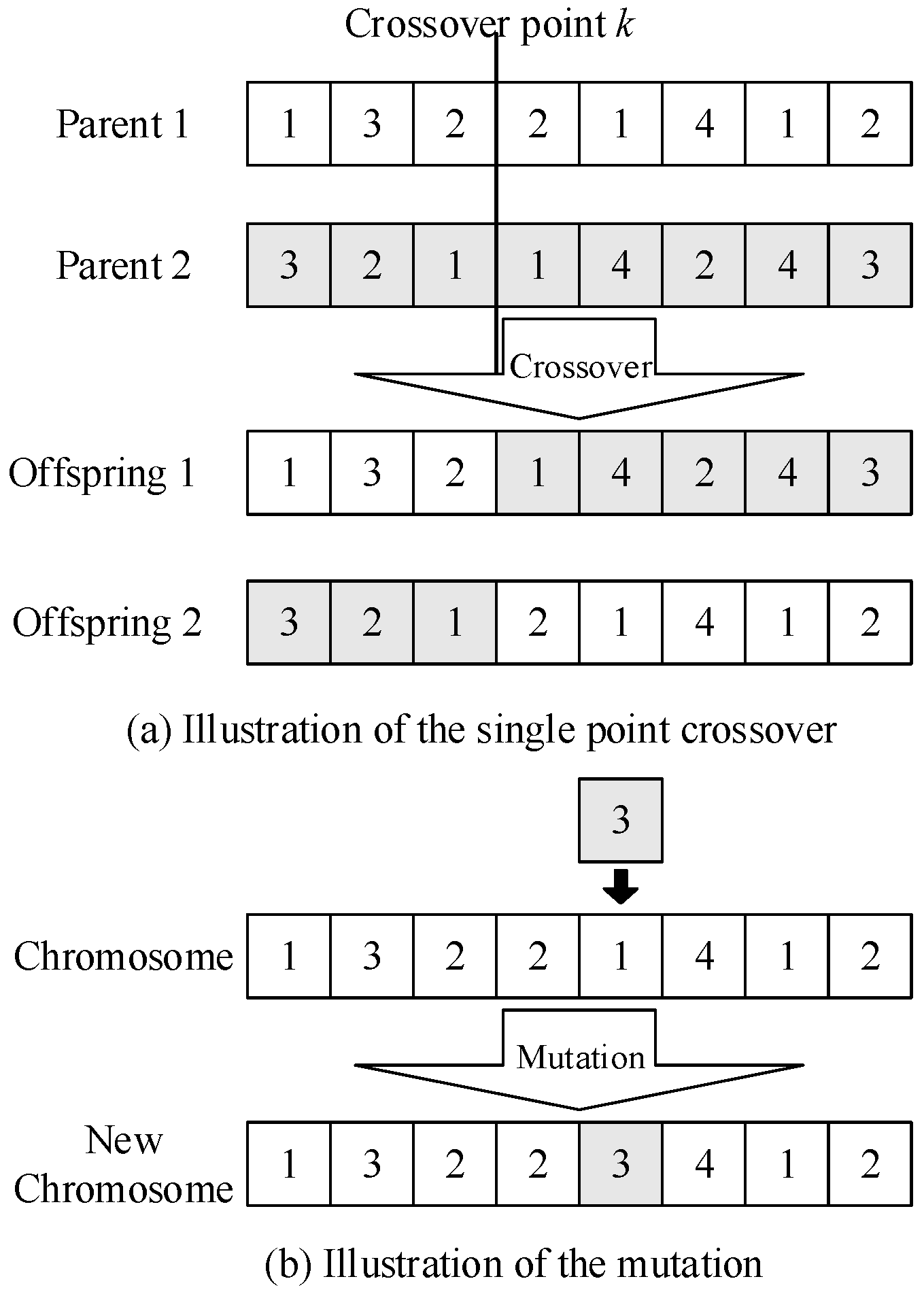
3.4.2. Crossover
3.4.3. Mutation
3.5. Complete Algorithm
3.6. Computational Complexity
4. Experiments and Comparisons
4.1. Algorithms Configurations
4.2. Experimental Results and Comparisons
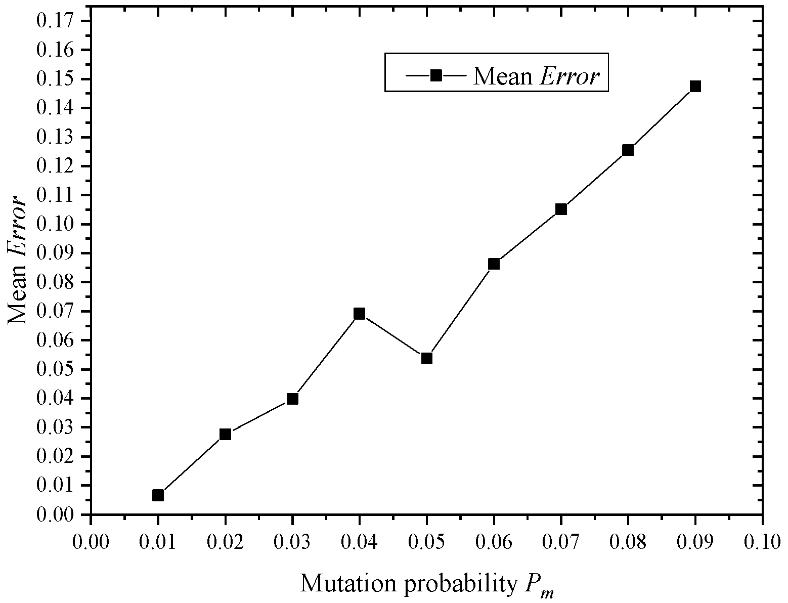
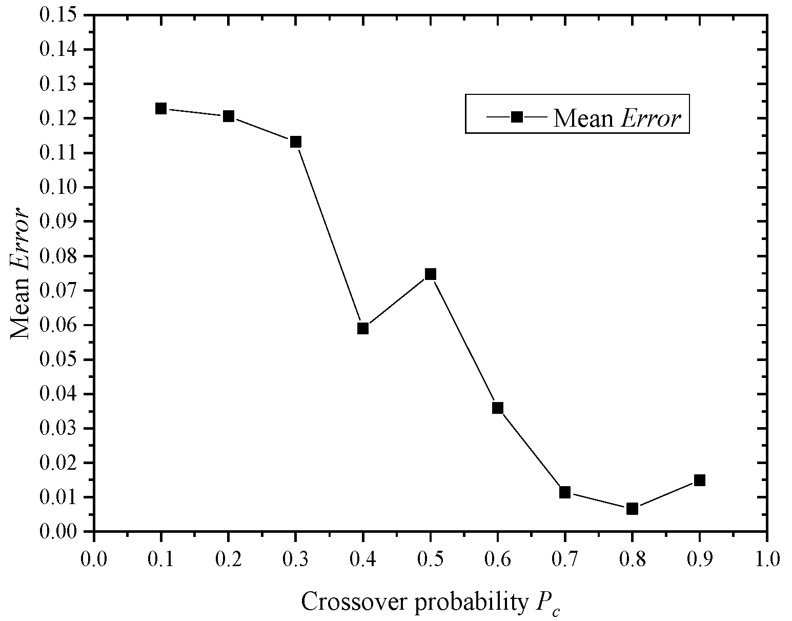
4.3. Effects of Parameters
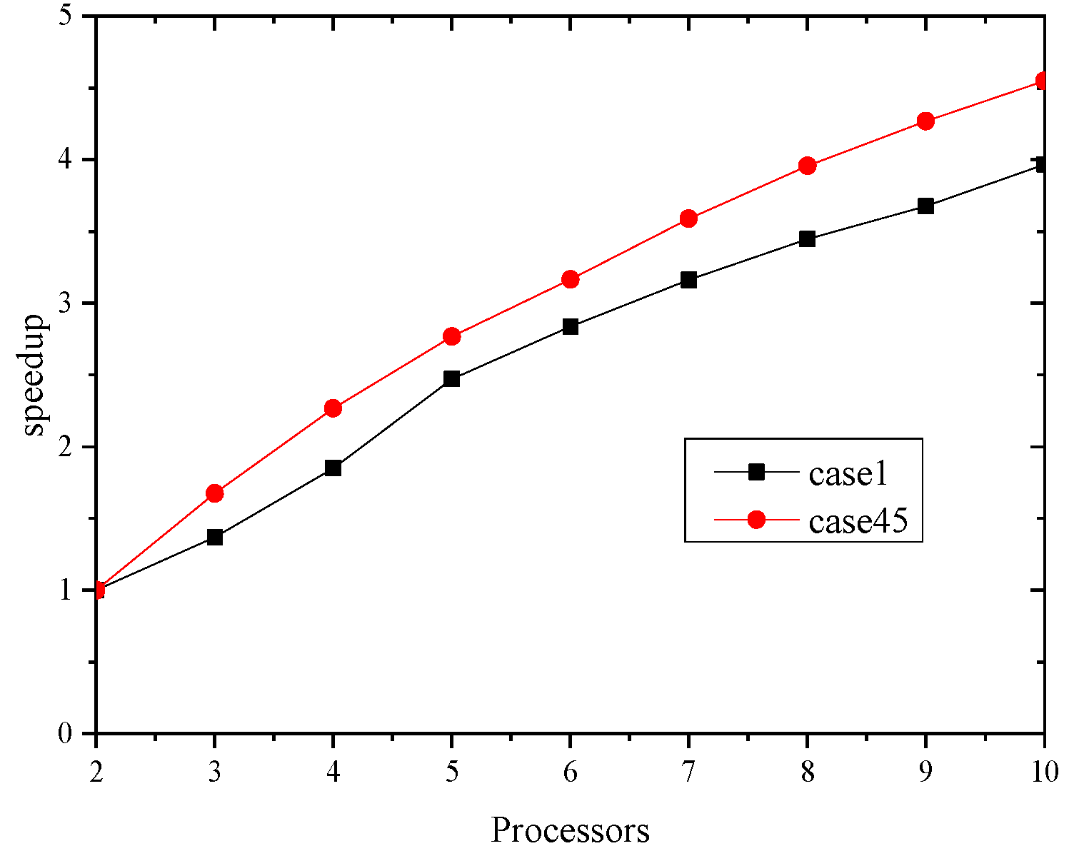
4.4. Speedup Ratio
5. Conclusions
Author Contributions
Funding
Acknowledgments
Conflicts of Interest
Nomenclature
| DGA | distributed genetic algorithm |
| EEC | energy efficient coverage |
| WSN | wireless sensor networks |
| D | the number of sensor nodes |
| M | the number of disjoint subsets |
| K | the upper bound of the disjoint sets number |
| N | the number of chromosomes |
| pc | crossover probability |
| pm | mutation probability |
References
- Guevara, J.; Barrero, F.; Vargas, E.; Becerra, J.; Toral, S. Environmental wireless sensor network for road traffic applications. IET Intell. Transp. Syst. 2012, 6, 177–186. [Google Scholar] [CrossRef]
- Wang, C.; Guo, S.; Yang, Y. An optimization framework for mobile data collection in energy-harvesting wireless sensor networks. IEEE Trans. Parallel Distrib. Syst. 2016, 15, 2969–2986. [Google Scholar] [CrossRef]
- Martinez, K.; Hart, J.K.; Ong, R. Environmental sensor networks. IEEE Comput. Soc. 2004, 37, 50–56. [Google Scholar] [CrossRef]
- Yahya, A.; Islam, S.; Akhunzada, A.; Ahmed, G.; Shamshirband, S.; Lloret, J. Towards efficient sink mobility in underwater wireless sensor networks. Energies 2018, 11, 1471. [Google Scholar] [CrossRef]
- Al-Jaoufi, M.A.A.; Liu, Y.; Zhang, Z.J. An active defense model with low power consumption and deviation for wireless sensor networks utilizing evolutionary game theory. Energies 2018, 11, 1281. [Google Scholar] [CrossRef]
- Shehadeh, H.A.; Idris, M.Y.I.; Ahmedy, I.; Ramli, R.; Noor, N.M. The multi-objective optimization algorithm based on sperm fertilization procedure (MOSFP) method for solving wireless sensor networks optimization problems in smart grid applications. Energies 2018, 11, 97. [Google Scholar] [CrossRef]
- Marzband, M.; Azarinejadian, F.; Savaghebi, M.; Pouresmaeil, E.; Guerrero, J.M.; Lightbody, G. Smart transactive energy framework in grid-connected multiple home microgrids under independent and coalition operations. Renew. Energy 2018, 126, 95–106. [Google Scholar] [CrossRef]
- Marzband, M.; Fouladfar, M.H.; Akorede, M.F.; Lightbody, G.; Pouresmaeil, E. Framework for smart transactive energy in home-microgrids considering coalition formation and demand side management. Sustain. Cities Soc. 2018, 40, 136–154. [Google Scholar] [CrossRef]
- Tavakoli, M.; Shokridehaki, F.; Akorede, M.F.; Marzband, M.; Vechiu, I.; Pouresmaeil, E. CVaR-based energy management scheme for optimal resilience and operational cost in commercial building microgrids. Int. J. Electr. Power Energy Syst. 2018, 100, 1–9. [Google Scholar] [CrossRef]
- Marzband, M.; Javadi, M.; Pourmousavi, S.A.; Lightbody, G. An advanced retail electricity market for active distribution systems and home microgrid interoperability based on game theory. Electr. Power Syst. Res. 2018, 157, 187–199. [Google Scholar] [CrossRef]
- Tavakoli, M.; Shokridehaki, F.; Marzband, M.; Godina, R.; Pouresmaeil, E. A two stage hierarchical control approach for the optimal energy management in commercial building microgrids based on local wind power and PEVs. Sustain. Cities Soc. 2018, 41, 332–340. [Google Scholar] [CrossRef]
- Marzband, M.; Sumper, A.; Domínguez-García, J.L.; Gumara-Ferreta, R. Experimental validation of a real time energy management system for microgrids in islanded mode using a local day-ahead electricity market and MINLP. Energy Convers. Manag. 2013, 76, 314–322. [Google Scholar] [CrossRef]
- Rajendran, V.; Obraczka, K.; Garcia-Luna-Aceves, J.J. Energy-efficient collision-free medium access control for wireless sensor networks. Wirel. Netw. 2006, 12, 63–78. [Google Scholar] [CrossRef]
- Chlamtac, I.; Petrioli, C.; Redi, J. Energy-conserving access protocols for identification networks. IEEE/ACM Trans. Netw. 1999, 7, 51–59. [Google Scholar] [CrossRef]
- Stine, J.; Veciana, G. Improving energy efficiency of centrally controlled wireless data networks. Wirel. Netw. 2002, 8, 681–700. [Google Scholar] [CrossRef]
- Huang, C.F.; Tseng, Y.C. A survey of solutions to the coverage problems in wireless sensor networks. J. Internet Technol. 2005, 6, 1–8. [Google Scholar]
- Ammari, H.M. Investigating the energy sink-hole problem in connected-covered wireless sensor networks. IEEE Trans. Comput. 2014, 63, 2729–2742. [Google Scholar] [CrossRef]
- Cardei, M.; Wu, J. Energy-efficient coverage problems in wireless ad-hoc sensor networks. Comput. Commun. 2006, 29, 413–420. [Google Scholar] [CrossRef]
- Tian, D.; Georganas, N.D. A node scheduling scheme for energy conservation in large wireless sensor networks. Wirel. Commun. Mob. Comput. 2003, 3, 271–290. [Google Scholar] [CrossRef]
- Zhan, Z.H.; Zhang, J.; Fan, Z. Solving the optimal coverage problem in wireless sensor networks using evolutionary computation algorithms. In Proceedings of the International Conference on Simulated Evolution and Learning, Kanpur, India, 1–4 December 2010; pp. 166–176. [Google Scholar]
- Slijepcevic, S.; Potkonjak, M. Power efficient organization of wireless sensor networks. In Proceedings of the IEEE International Conference on Communications, Helsinki, Finland, 11–14 June 2001. [Google Scholar]
- Cardei, M.; MacCallum, D.; Cheng, X.; Min, M.; Jia, X.; Li, D.; Du, D.Z. Wireless sensor networks with energy efficient organization. J. Interconnect. Netw. 2002, 3, 213–229. [Google Scholar] [CrossRef]
- Zhang, X.Y.; Zhang, J.; Gong, Y.J.; Zhan, Z.H.; Chen, W.N.; Li, Y. Kuhn-munkres parallel genetic algorithm for the set cover problem and its application to large-scale wireless sensor networks. IEEE Trans. Evol. Comput. 2016, 20, 695–710. [Google Scholar] [CrossRef]
- Li, X.Y.; Wan, P.J.; Frieder, O. Coverage in wireless and ad-hoc sensor networks. IEEE Trans. Comput. 2003, 52, 753–762. [Google Scholar] [CrossRef]
- Lai, C.C.; Ting, C.K.; Ko, R.S. An effective genetic algorithm to improve wireless sensor network lifetime for large-scale surveillance applications. In Proceedings of the IEEE Congress on Evolutionary Computation, Singapore, 25–28 September 2007. [Google Scholar]
- Kampelis, N.; Tsekeri, E.; Kolokotsa, D.; Kalaitzakis, K.; Isidori, D.; Cristina, C. 3 Development of demand response energy management optimization at building and district levels using genetic algorithm and artificial neural network modelling power predictions. Energies 2018, 11, 3012. [Google Scholar] [CrossRef]
- Liu, X.F.; Zhan, Z.H.; Deng, D.; Li, Y.; Gu, T.L.; Zhang, J. An energy efficient ant colony system for virtual machine placement in cloud computing. IEEE Trans. Evol. Comput. 2018, 22, 113–128. [Google Scholar] [CrossRef]
- Chen, Z.G.; Zhan, Z.H.; Lin, Y.; Gong, Y.J.; Gu, T.L.; Zhao, F.; Yuan, H.Q.; Chen, X.; Li, Q.; Zhang, J. Multiobjective cloud workflow scheduling: A multiple populations ant colony system approach. IEEE Trans. Cybern. 2018. [Google Scholar] [CrossRef] [PubMed]
- Li, Y.H.; Zhan, Z.H.; Lin, S.J.; Zhang, J.; Luo, X.N. Competitive and cooperative particle swarm optimization with information sharing mechanism for global optimization problems. Inf. Sci. 2015, 293, 370–382. [Google Scholar] [CrossRef]
- Liu, X.F.; Zhan, Z.H.; Gao, Y.; Zhang, J.; Kwong, S.; Zhang, J. Coevolutionary particle swarm optimization with bottleneck objective learning strategy for many-objective optimization. IEEE Trans. Evol. Comput. 2018. [Google Scholar] [CrossRef]
- Wang, Z.J.; Zhan, Z.H.; Lin, Y.; Yu, W.J.; Yuan, H.Q.; Gu, T.L.; Kwong, S.; Zhang, J. Dual-strategy differential evolution with affinity propagation clustering for multimodal optimization problems. IEEE Trans. Evol. Comput. 2018, 22, 894–908. [Google Scholar] [CrossRef]
- Liu, X.F.; Zhan, Z.H.; Lin, Y.; Chen, W.N.; Gong, Y.J.; Gu, T.L.; Yuan, H.Q.; Zhang, J. Historical and heuristic based adaptive differential evolution. IEEE Trans. Syst. Man Cybern. Syst. 2018. [Google Scholar] [CrossRef]
- Zhan, Z.H.; Zhang, J.; Du, K.J.; Xiao, J. Extended binary particle swarm optimization approach for disjoint set covers problem in wireless sensor networks. In Proceedings of the IEEE Conference on Technologies and Applications of Artificial Intelligence, Tainan, Taiwan, 16–18 November 2012. [Google Scholar]
- Lin, Y.; Zhang, J.; Chung, H.S.H.; Ip, W.H.; Li, Y.; Shi, Y.H. An ant colony optimization approach for maximizing the lifetime of heterogeneous wireless sensor networks. IEEE Trans. Syst. Man Cybern. Part C (Appl. Rev.) 2012, 42, 408–420. [Google Scholar] [CrossRef]
- Yang, Q.Q.; He, S.B.; Li, J.K.; Chen, J.M.; Sun, Y.X. Energy-efficient probabilistic area coverage in wireless sensor networks. IEEE Trans. Veh. Technol. 2015, 64, 367–377. [Google Scholar] [CrossRef]
- Lee, J.W.; Choi, B.S.; Lee, J.J. Energy-efficient coverage of wireless sensor networks using ant colony optimization with three types of pheromones. IEEE Trans. Ind. Informat. 2011, 7, 419–427. [Google Scholar] [CrossRef]
- Lee, J.W.; Lee, J.Y.; Lee, J.J. Jenga-inspired optimization algorithm for energy-efficient coverage of unstructured WSNs. IEEE Wirel. Commun. Lett. 2013, 2, 34–37. [Google Scholar] [CrossRef]
- Zhan, Z.H.; Liu, X.F.; Zhang, H.; Yu, Z.; Weng, J.; Li, Y.; Gu, T.; Zhang, J. Cloudde: A heterogeneous differential evolution algorithm and its distributed cloud version. IEEE Trans. Parallel Distrib. Syst. 2017, 28, 704–716. [Google Scholar] [CrossRef]
- Shen, M.; Zhan, Z.H.; Chen, W.N.; Gong, Y.J.; Zhang, J.; Li, Y. Bi-velocity discrete particle swarm optimization and its application to multicast routing problem in communication networks. IEEE Trans. Ind. Electron. 2014, 61, 7141–7151. [Google Scholar] [CrossRef]
- Zhan, Z.H.; Liu, X.F.; Gong, Y.J.; Zhang, J.; Chung, H.S.H.; Li, Y. Cloud computing resource scheduling and a survey of its evolutionary approaches. ACM Comput. Surv. 2015, 47, 1–33. [Google Scholar] [CrossRef]
- Liu, X.F.; Zhan, Z.H.; Zhang, J. Neural network for change direction prediction in dynamic optimization. IEEE Access 2018, 6, 72649–72662. [Google Scholar] [CrossRef]
- Zhan, Z.H.; Li, J.; Cao, J.; Zhang, J.; Chung, H.; Shi, Y.H. Multiple populations for multiple objectives: A coevolutionary technique for solving multiobjective optimization problems. IEEE Trans. Cybern. 2013, 43, 445–463. [Google Scholar] [CrossRef] [PubMed]


| Parameter | Configuration |
|---|---|
| N | 40 |
| Generation | 200 |
| pc | 0.8 |
| pm | 0.01 |
| Case No. | Topology | Upper Bound K | All Combinations | Mean Disjoint Set Number M | Error | |||||
|---|---|---|---|---|---|---|---|---|---|---|
| Node | Range | GAMDSC | BPSO | DGA | GAMDSC | BPSO | DGA | |||
| 1 | 100 | 8 | 2 | 2^100 | 2.000 | 2.000 | 2.000 | 0.000 | 0.000 | 0.000 |
| 2 | 2 | 2^100 | 2.000 | 2.000 | 2.000 | 0.000 | 0.000 | 0.000 | ||
| 3 | 2 | 2^100 | 2.000 | 2.000 | 2.000 | 0.000 | 0.000 | 0.000 | ||
| 4 | 100 | 10 | 2 | 2^100 | 2.000 | 2.000 | 2.000 | 0.000 | 0.000 | 0.000 |
| 5 | 2 | 2^100 | 2.000 | 2.000 | 2.000 | 0.000 | 0.000 | 0.000 | ||
| 6 | 2 | 2^100 | 2.000 | 2.000 | 2.000 | 0.000 | 0.000 | 0.000 | ||
| 7 | 100 | 12 | 2 | 2^100 | 2.000 | 2.000 | 2.000 | 0.000 | 0.000 | 0.000 |
| 8 | 2 | 2^100 | 2.000 | 2.000 | 2.000 | 0.000 | 0.000 | 0.000 | ||
| 9 | 4 | 4^100 | 3.900 | 3.600 | 4.000 | 0.025 | 0.100 | 0.000 | ||
| 10 | 150 | 8 | 2 | 2^150 | 2.000 | 2.000 | 2.000 | 0.000 | 0.000 | 0.000 |
| 11 | 2 | 2^150 | 2.000 | 2.000 | 2.000 | 0.000 | 0.000 | 0.000 | ||
| 12 | 2 | 2^150 | 2.000 | 2.000 | 2.000 | 0.000 | 0.000 | 0.000 | ||
| 13 | 150 | 10 | 3 | 3^150 | 3.000 | 3.000 | 3.000 | 0.000 | 0.000 | 0.000 |
| 14 | 4 | 4^150 | 3.500 | 3.200 | 4.000 | 0.125 | 0.200 | 0.000 | ||
| 15 | 3 | 3^150 | 3.000 | 3.000 | 3.000 | 0.000 | 0.000 | 0.000 | ||
| 16 | 150 | 12 | 5 | 5^150 | 4.200 | 5.000 | 5.000 | 0.000 | 0.000 | 0.000 |
| 17 | 3 | 3^150 | 3.000 | 3.000 | 3.000 | 0.000 | 0.000 | 0.000 | ||
| 18 | 4 | 4^150 | 3.800 | 4.000 | 4.000 | 0.050 | 0.000 | 0.000 | ||
| 19 | 200 | 8 | 2 | 2^200 | 2.000 | 2.000 | 2.000 | 0.000 | 0.000 | 0.000 |
| 20 | 2 | 2^200 | 2.000 | 2.000 | 2.000 | 0.000 | 0.000 | 0.000 | ||
| 21 | 3 | 3^200 | 3.000 | 3.000 | 3.000 | 0.000 | 0.000 | 0.000 | ||
| 22 | 200 | 10 | 3 | 3^200 | 3.000 | 3.000 | 3.000 | 0.000 | 0.000 | 0.000 |
| 23 | 4 | 4^200 | 3.500 | 3.300 | 4.000 | 0.125 | 0.175 | 0.000 | ||
| 24 | 5 | 5^200 | 5.000 | 4.600 | 5.000 | 0.000 | 0.080 | 0.000 | ||
| 25 | 200 | 12 | 7 | 7^200 | 5.900 | 6.200 | 7.000 | 0.157 | 0.114 | 0.000 |
| 26 | 8 | 8^200 | 7.200 | 6.600 | 8.000 | 0.100 | 0.175 | 0.000 | ||
| 27 | 9 | 9^200 | 7.300 | 7.500 | 9.000 | 0.189 | 0.166 | 0.000 | ||
| 28 | 250 | 8 | 3 | 3^250 | 3.000 | 3.000 | 3.000 | 0.000 | 0.000 | 0.000 |
| 29 | 3 | 3^250 | 3.000 | 3.000 | 3.000 | 0.000 | 0.000 | 0.000 | ||
| 30 | 5 | 5^250 | 4.900 | 4.100 | 5.000 | 0.020 | 0.180 | 0.000 | ||
| 31 | 250 | 10 | 5 | 5^250 | 5.000 | 5.000 | 5.000 | 0.000 | 0.000 | 0.000 |
| 32 | 7 | 7^250 | 6.300 | 6.600 | 7.000 | 0.100 | 0.057 | 0.000 | ||
| 33 | 6 | 6^250 | 5.700 | 5.900 | 6.000 | 0.050 | 0.016 | 0.000 | ||
| 34 | 250 | 12 | 11 | 11^250 | 9.900 | 9.700 | 10.00 | 0.100 | 0.118 | 0.091 |
| 35 | 9 | 9^250 | 8.600 | 8.700 | 9.000 | 0.044 | 0.033 | 0.000 | ||
| 36 | 8 | 8^250 | 8.000 | 8.000 | 8.000 | 0.000 | 0.000 | 0.000 | ||
| 37 | 300 | 8 | 6 | 6^300 | 6.000 | 6.000 | 6.000 | 0.000 | 0.000 | 0.000 |
| 38 | 3 | 3^300 | 3.000 | 3.000 | 3.000 | 0.000 | 0.000 | 0.000 | ||
| 39 | 5 | 5^300 | 5.000 | 5.000 | 5.000 | 0.000 | 0.000 | 0.000 | ||
| 40 | 300 | 10 | 7 | 7^300 | 7.000 | 6.600 | 7.000 | 0.000 | 0.057 | 0.000 |
| 41 | 7 | 7^300 | 7.000 | 6.800 | 7.000 | 0.000 | 0.029 | 0.000 | ||
| 42 | 9 | 9^300 | 8.300 | 7.400 | 8.400 | 0.100 | 0.178 | 0.067 | ||
| 43 | 300 | 12 | 11 | 11^300 | 10.60 | 10.00 | 10.10 | 0.036 | 0.091 | 0.082 |
| 44 | 12 | 12^300 | 10.80 | 10.90 | 11.30 | 0.100 | 0.092 | 0.058 | ||
| 45 | 9 | 9^300 | 8.800 | 8.600 | 9.000 | 0.022 | 0.044 | 0.000 | ||
| Processors | 2 | 3 | 4 | 5 | 6 | 7 | 8 | 9 | 10 | |
|---|---|---|---|---|---|---|---|---|---|---|
| Case No. | ||||||||||
| 1 | 101.53 | 74.26 | 54.91 | 41.07 | 35.78 | 32.09 | 29.45 | 27.62 | 25.59 | |
| 2 | 123.24 | 90.50 | 71.44 | 57.29 | 53.83 | 50.38 | 46.36 | 42.50 | 39.85 | |
| 3 | 133.24 | 96.64 | 77.30 | 69.96 | 62.33 | 59.80 | 54.87 | 50.64 | 48.59 | |
| 4 | 116.77 | 85.19 | 70.76 | 63.55 | 56.58 | 52.39 | 48.84 | 43.78 | 39.49 | |
| 5 | 147.74 | 100.36 | 87.53 | 73.46 | 65.86 | 59.73 | 53.92 | 50.05 | 48.74 | |
| 6 | 132.90 | 95.19 | 83.47 | 71.41 | 64.11 | 58.53 | 53.29 | 49.39 | 47.98 | |
| 7 | 158.20 | 107.27 | 88.06 | 76.62 | 68.54 | 63.16 | 56.23 | 52.28 | 49.77 | |
| 8 | 144.34 | 103.50 | 86.77 | 77.06 | 68.96 | 62.38 | 57.05 | 52.48 | 49.21 | |
| 9 | 258.93 | 169.97 | 130.72 | 101.29 | 89.81 | 80.90 | 72.86 | 65.29 | 61.41 | |
| 10 | 188.84 | 120.19 | 93.42 | 82.38 | 71.84 | 64.46 | 56.94 | 50.00 | 47.80 | |
| 11 | 178.36 | 118.36 | 93.21 | 81.42 | 70.64 | 63.89 | 56.37 | 49.08 | 46.32 | |
| 12 | 206.96 | 128.08 | 98.24 | 84.18 | 73.99 | 65.19 | 58.03 | 53.99 | 50.02 | |
| 13 | 253.12 | 142.81 | 110.06 | 94.95 | 84.88 | 77.37 | 73.10 | 69.00 | 67.81 | |
| 14 | 321.11 | 205.79 | 158.70 | 139.89 | 126.43 | 113.42 | 100.45 | 90.67 | 84.10 | |
| 15 | 272.37 | 164.89 | 142.60 | 123.77 | 105.18 | 90.94 | 78.09 | 69.07 | 63.82 | |
| 16 | 386.60 | 267.58 | 201.73 | 175.17 | 139.95 | 123.07 | 110.80 | 100.43 | 94.91 | |
| 17 | 284.46 | 214.86 | 151.65 | 123.60 | 104.80 | 90.44 | 88.16 | 79.07 | 73.94 | |
| 18 | 308.81 | 223.46 | 176.00 | 143.88 | 122.89 | 110.73 | 97.94 | 89.17 | 82.92 | |
| 19 | 267.02 | 178.39 | 145.59 | 123.05 | 101.54 | 90.55 | 81.90 | 74.43 | 69.95 | |
| 20 | 284.36 | 193.04 | 152.46 | 125.60 | 104.22 | 95.95 | 86.24 | 79.70 | 74.18 | |
| 21 | 349.97 | 249.11 | 185.50 | 145.96 | 120.79 | 108.76 | 96.98 | 88.63 | 83.98 | |
| 22 | 351.04 | 246.52 | 189.91 | 156.78 | 136.28 | 122.45 | 109.88 | 102.45 | 96.40 | |
| 23 | 445.03 | 323.38 | 236.05 | 196.38 | 167.02 | 147.60 | 129.79 | 120.12 | 115.23 | |
| 24 | 533.63 | 354.34 | 286.87 | 242.26 | 219.79 | 189.75 | 162.89 | 147.38 | 139.96 | |
| 25 | 627.89 | 457.94 | 346.32 | 271.15 | 224.81 | 198.03 | 176.26 | 166.13 | 157.15 | |
| 26 | 682.48 | 475.31 | 363.82 | 288.01 | 236.70 | 209.82 | 189.36 | 175.76 | 170.80 | |
| 27 | 744.13 | 501.08 | 389.95 | 305.20 | 248.85 | 228.48 | 216.66 | 206.95 | 199.67 | |
| 28 | 436.20 | 281.56 | 233.98 | 198.82 | 165.39 | 145.43 | 134.42 | 119.83 | 112.49 | |
| 29 | 412.85 | 265.29 | 215.59 | 194.15 | 169.05 | 148.05 | 133.49 | 120.88 | 112.55 | |
| 30 | 563.58 | 378.05 | 295.38 | 245.90 | 202.31 | 171.01 | 156.44 | 148.80 | 141.01 | |
| 31 | 591.87 | 380.09 | 308.38 | 254.81 | 214.68 | 189.08 | 169.17 | 161.44 | 156.99 | |
| 32 | 680.79 | 485.09 | 354.86 | 278.55 | 236.14 | 201.17 | 188.06 | 179.64 | 173.99 | |
| 33 | 625.32 | 454.75 | 336.59 | 257.97 | 224.26 | 200.25 | 184.99 | 171.09 | 166.34 | |
| 34 | 1687.20 | 1153.09 | 916.81 | 799.34 | 684.47 | 585.99 | 509.48 | 451.04 | 424.53 | |
| 35 | 871.04 | 578.18 | 449.48 | 388.74 | 343.93 | 309.37 | 264.36 | 241.62 | 225.94 | |
| 36 | 778.21 | 560.31 | 401.16 | 372.50 | 327.59 | 290.98 | 262.23 | 236.73 | 220.14 | |
| 37 | 1014.52 | 697.61 | 580.35 | 502.69 | 439.96 | 384.46 | 321.52 | 288.86 | 272.87 | |
| 38 | 836.59 | 580.41 | 446.17 | 385.78 | 332.98 | 294.35 | 251.36 | 222.99 | 210.33 | |
| 39 | 958.63 | 635.55 | 528.04 | 418.04 | 350.24 | 303.71 | 264.91 | 244.66 | 233.68 | |
| 40 | 1302.70 | 825.53 | 671.78 | 598.59 | 522.32 | 451.68 | 400.26 | 363.22 | 342.84 | |
| 41 | 1412.63 | 915.99 | 732.56 | 603.58 | 508.87 | 449.00 | 414.48 | 382.68 | 367.28 | |
| 42 | 2297.81 | 1542.50 | 1208.43 | 1048.97 | 915.04 | 801.93 | 713.63 | 638.74 | 586.86 | |
| 43 | 2416.68 | 1651.56 | 1217.74 | 1082.13 | 951.69 | 837.25 | 732.56 | 651.62 | 606.25 | |
| 44 | 2530.80 | 1754.12 | 1317.12 | 1181.00 | 1008.09 | 886.37 | 782.98 | 696.21 | 634.14 | |
| 45 | 1916.47 | 1144.10 | 845.52 | 692.63 | 605.70 | 534.16 | 484.21 | 449.11 | 421.29 | |
© 2018 by the authors. Licensee MDPI, Basel, Switzerland. This article is an open access article distributed under the terms and conditions of the Creative Commons Attribution (CC BY) license (http://creativecommons.org/licenses/by/4.0/).
Share and Cite
Wang, Z.-J.; Zhan, Z.-H.; Zhang, J. Solving the Energy Efficient Coverage Problem in Wireless Sensor Networks: A Distributed Genetic Algorithm Approach with Hierarchical Fitness Evaluation. Energies 2018, 11, 3526. https://doi.org/10.3390/en11123526
Wang Z-J, Zhan Z-H, Zhang J. Solving the Energy Efficient Coverage Problem in Wireless Sensor Networks: A Distributed Genetic Algorithm Approach with Hierarchical Fitness Evaluation. Energies. 2018; 11(12):3526. https://doi.org/10.3390/en11123526
Chicago/Turabian StyleWang, Zi-Jia, Zhi-Hui Zhan, and Jun Zhang. 2018. "Solving the Energy Efficient Coverage Problem in Wireless Sensor Networks: A Distributed Genetic Algorithm Approach with Hierarchical Fitness Evaluation" Energies 11, no. 12: 3526. https://doi.org/10.3390/en11123526
APA StyleWang, Z.-J., Zhan, Z.-H., & Zhang, J. (2018). Solving the Energy Efficient Coverage Problem in Wireless Sensor Networks: A Distributed Genetic Algorithm Approach with Hierarchical Fitness Evaluation. Energies, 11(12), 3526. https://doi.org/10.3390/en11123526