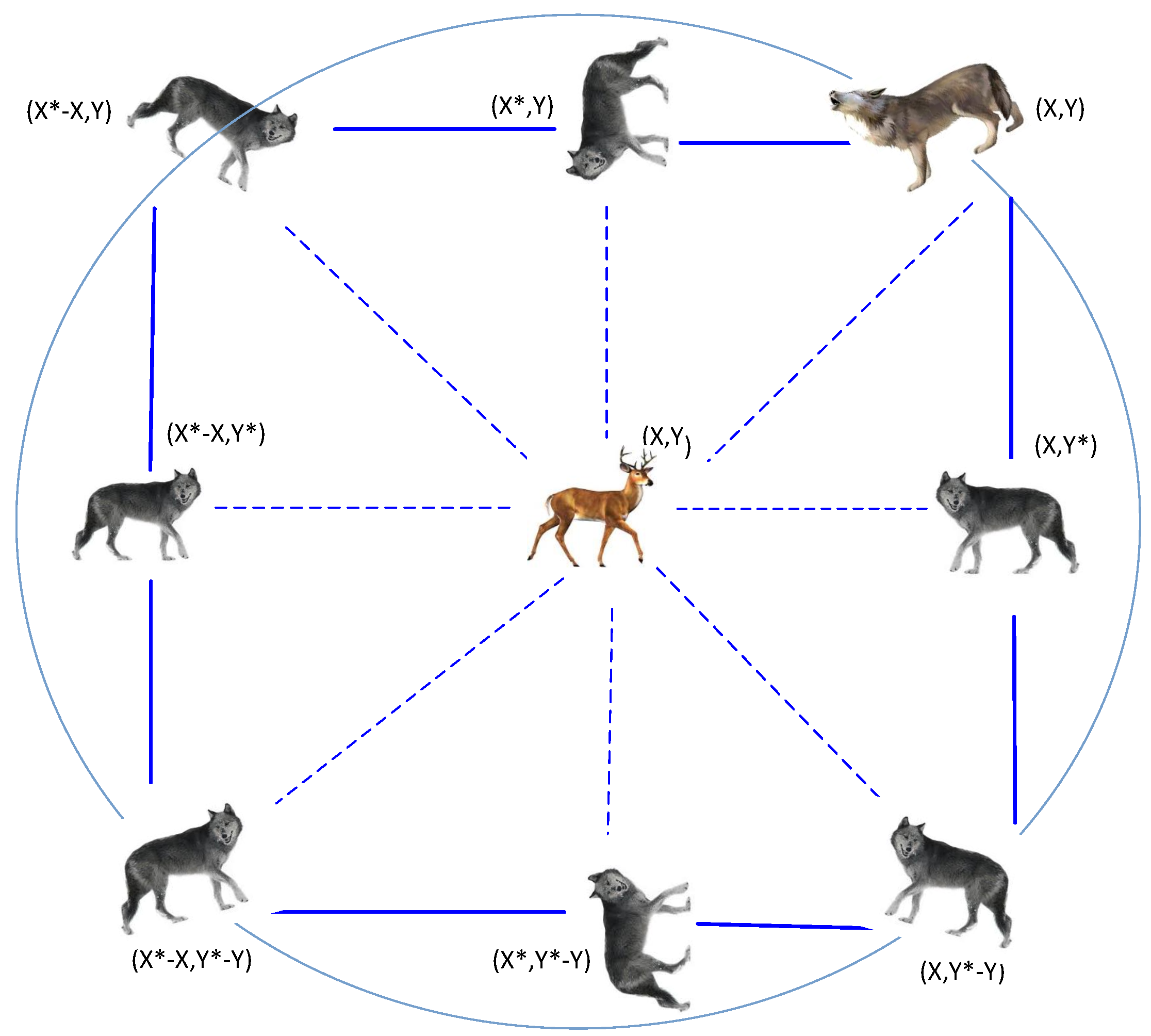
Article

Short-Term Electric Load and Price Forecasting Using Enhanced Extreme Learning Machine Optimization in Smart Grids

1
Department of Computer Science, COMSATS University Islamabad, Islamabad 44000, Pakistan
2
College of Computer and Information Systems, Al Yamamah University, Riyadh 11512, Saudi Arabia
3
Computer Engineering Department, College of Computer and Information Sciences, King Saud University, Riyadh 11543, Saudi Arabia
*
Authors to whom correspondence should be addressed.
Energies 2019, 12(5), 866; https://doi.org/10.3390/en12050866
Submission received: 1 February 2019 / Revised: 20 February 2019 / Accepted: 22 February 2019 / Published: 5 March 2019

Abstract

:
A Smart Grid (SG) is a modernized grid to provide efficient, reliable and economic energy to the consumers. Energy is the most important resource in the world. An efficient energy distribution is required as smart devices are increasing dramatically. The forecasting of electricity consumption is supposed to be a major constituent to enhance the performance of SG. Various learning algorithms have been proposed to solve the forecasting problem. The sole purpose of this work is to predict the price and load efficiently. The first technique is Enhanced Logistic Regression (ELR) and the second technique is Enhanced Recurrent Extreme Learning Machine (ERELM). ELR is an enhanced form of Logistic Regression (LR), whereas, ERELM optimizes weights and biases using a Grey Wolf Optimizer (GWO). Classification and Regression Tree (CART), Relief-F and Recursive Feature Elimination (RFE) are used for feature selection and extraction. On the basis of selected features, classification is performed using ELR. Cross validation is done for ERELM using Monte Carlo and K-Fold methods. The simulations are performed on two different datasets. The first dataset, i.e., UMass Electric Dataset is multi-variate while the second dataset, i.e., UCI Dataset is uni-variate. The first proposed model performed better with UMass Electric Dataset than UCI Dataset and the accuracy of second model is better with UCI than UMass. The prediction accuracy is analyzed on the basis of four different performance metrics: Mean Absolute Percentage Error (MAPE), Mean Absolute Error (MAE), Mean Square Error (MSE) and Root Mean Square Error (RMSE). The proposed techniques are then compared with four benchmark schemes. The comparison is done to verify the adaptivity of the proposed techniques. The simulation results show that the proposed techniques outperformed benchmark schemes. The proposed techniques efficiently increased the prediction accuracy of load and price. However, the computational time is increased in both scenarios. ELR achieved almost 5% better results than Convolutional Neural Network (CNN) and almost 3% than LR. While, ERELM achieved almost 6% better results than ELM and almost 5% than RELM. However, the computational time is almost 20% increased with ELR and 50% with ERELM. Scalability is also addressed for the proposed techniques using half-yearly and yearly datasets. Simulation results show that ELR gives 5% better results while, ERELM gives 6% better results when used for yearly dataset.

1. Introduction

For electricity generation and distribution, Traditional Grids (TGs) are used. The infrastructure of TG is getting obsolete, which results in energy loss and less efficient output. Due to the usage of outdated infrastructure, intensive power losses are being faced. This intensive power loss leads to load shedding, which is one of the major issues of today’s world [1]. TGs use fossil fuels like coal, petrol, diesel, etc., for the combustion process of turbines. The extensive use of fossil fuels lead to natural resource depletion and increase in pollution. The literature has suggested to use Renewable Energy Sources (RES) and to modify the existing TGs by incorporating the latest technologies and updated infrastructure to overcome these issues. The new and modified form of TG is the Smart Grid (SG) [2]. The Information and Communication Technology (ICT) is integrated with TG to make SG. It provides bi-directional communication between consumers and utility. It monitors, protects and optimizes the generation, distribution and consumption of electric energy. It incorporates the latest technologies in TG: technical, control and communication technologies, to enable efficient energy transmission. With an ever increasing dilemma of energy shortage and cost inflation, people are attracted towards the SG. It provides the consumers with a reliable, economical, sustainable, secure and efficient energy as it uses intelligent methods. In SG, Demand Side Management (DSM) is used, which encourages the consumers to efficiently optimize the energy usage. DSM allows efficient load utilization by shifting maximum load from on-peak hours to off-peak hours. Thus, it reduced the cost of electricity. The differences between TG and SG are summarized in Table 1 [3].
Data analytics is the phenomenon of dealing with big data obtained from different sources. Big data is the term used for the datasets having large volume, velocity, variety and veracity. It has the problem of extreme complexity which makes the processing of data difficult. Data analytics techniques are the necessity for the processing of big data. Data analytics can be used in a number of fields. For example, handling the financial details of customers by a bank, dealing with the flight details of different passengers by an airline company, dealing with the electricity load and price forecasting of consumers, etc. In SG, data analytics is used to minimize the electricity cost and to improve the service quality of energy utilities. It is also used to predict the future patterns of electricity consumption. Forecasting is done to schedule the load consumption from on-peak hours to off-peak hours for next day, week or month to reduce the electricity cost and enhance user comfort [4].
The terms forecasting and prediction are used interchangeably in this article. The case with load and consumption is similar. The sole purpose of this work is to increase the accuracy of load and price forecasting. Two techniques are proposed to solve the aforementioned objectives, i.e., ELR and ERELM. Furthermore, two types of datasets are used, i.e., uni-variate and multi-variate. UCI is the uni-variate dataset. Uni-variate dataset contains one variable, i.e., load in this paper. However, real-time data has a number of variables. Thus, multi-variate dataset is required to handle multiple variables to achieve a better understanding. In this paper, multi-variate dataset, i.e., UMass Electric Dataset is used to predict the load and price. Two types of scenarios are considered in this paper, i.e., residential load and smart meters load. The proposed techniques outperformed existing techniques in terms of forecasting load and price. Consequently, energy prediction assists in energy management on the residential and utility side. List of abbreviations that are used in this paper is given in Table 2. Whereas, Table 3 shows complete list of symbols.
The rest of the paper is organized as: Section 2 deals with related work, Section 3 contains the detailed description of techniques used in this paper. Section 4 covers the proposed system models. Results and their discussion are given in Section 5, whereas Section 6 consists of evaluation of the proposed models using the performance metrics. Conclusion and future studies are discussed in Section 7.

1.1. Motivation

The authors in [5] used Multi Layer Perceptron (MLP) and Artificial Neural Network (ANN) to solve the load and price forecasting problem. We proposed an enhanced technique to increase the accuracy of load and price forecasting based on a modified loss function. In Reference [6], authors used ELM and RELM to predict electricity load. We proposed an enhanced technique to optimize weights and biases of network for efficient load forecasting. Furthermore, two scenarios are considered and two different types of datasets are used to predict the load and price efficiently.

1.2. Problem Statement

Data of SGs are increasing dramatically so an efficient technique is required to predict the load and price of electricity. Authors in [6] used Recurrent Extreme Learning Machine (RELM) to predict the electricity load. However, in RELM, weights and biases are randomly assigned which leads to drastic variations in prediction results. An enhanced technique is proposed to solve the aforesaid issue. In Reference [7], authors used Convolutional Neural Networks (CNNs) for predicting the energy demand. However, CNN involves tuning of a number of layers which makes it spatio-temporal complex.
In this paper, two enhanced techniques are proposed to increase the accuracy of load and price of electricity efficiently. Uni-variate and multi-variate datasets are used for both techniques. Furthermore, analysis of both residential and utility data is performed collectively.

1.3. Contributions

The following are the contributions of this paper:
  • Feature engineering is performed using Recursive Feature Elimination (RFE), Classification And Regression Technique (CART) and Relief-F
  • Two new classification techniques are proposed, i.e., Enhanced Logistic Regression (ELR) and Enhanced Recurrent Extreme Learning Machine (ERELM)
  • In ELR, the loss function of Logistic Regression (LR) is modified to increase the prediction accuracy
  • The Grey Wolf Optimizer (GWO) learning algorithm is used with Recurrent Extreme Learning Machine (RELM) to optimize weights and biases in order to improve the forecasting accuracy
  • The proposed techniques predict the electricity load and price efficiently
  • ELR is used to predict the load and price of a smart home, whereas ERELM is used for forecasting the load of smart meters
  • Cross validation is performed using K-Fold and Monte Carlo methods for assigning the fixed optimal values to weights and biases. This further increases the efficiency of GWO
  • The accuracy of the proposed techniques is evaluated using the performance metrics, i.e., Mean Absolute Error (MAE), Mean Square Error (MSE), Mean Absolute Percentage Error (MAPE) and Root Mean Square Error (RMSE)

2. Related Work

Many forecasting techniques have been used in the past for load and price forecasting. These techniques can be categorized in three main groups: data driven, classical and Artificial Intelligence (AI). Data driven techniques consider past data to predict the desired outcomes. Classical methods comprise of the statistical and mathematical methods like Autoregressive Integrated Moving Average (ARIMA), Seasonal Autoregressive Integrated Moving Average (SARIMA), Random Forest (RF), etc., whereas AI methods mimic the behaviour of biological neurons like Feed Forward Neural Network (FFNN), Convolutional Neural Network (CNN), Long Short Term Memory (LSTM), etc.

2.1. Electricity Load Forecasting

In Reference [8], behavioural analytics are performed using Bayesian network and Multi Layer Perceptron (MLP). A number of experiments were performed using the data obtainedfrom the smart meters. Both short-term and long-term forecasting was performed. In Reference [9], Multiple Linear Regression (MLR) is used for forecasting purpose. However, it has the limitation that it can not be used for long term prediction. The authors in [10] used residual network for forecasting load on the basis of weather data. The authors in [11] used Restricted Boltzmann Machine (RBM) to train the data and Rectified Linear Unit (ReLU) to predict the electricity load. In Reference [12], Discrete Wavelet Transform (DWT) and Inconsistency Rate (IR) methods are proposed to select the optimal features from the feature set which helps in dimensionality reduction. Sperm Whale Algorithm (SWA) helps to optimize the parameters of SVM. Authors in [13] proposed a model for Short Term Load Forecasting (STLF). Mutual Information (MI) is used for feature selection whereas, better forecasting results are achieved by modifying the Artificial Neural Network (ANN). In Reference [14], authors predicted 24 h ahead cooling load of buildings using deep learning. The results show that deep learning techniques enhanced the load prediction. Similarly in [15], authors used Recurrent Neural Network (RNN), which groups the consumers into pool of inputs. The proposed model is implemented using Tensorflow package and it achieved better results.
ELM is a generalized single hidden layer FFNN learning algorithm that is proposed by the authors in References [16,17]. It proved to be effective in both regression and classification methods. In References [18,19], authors used the NNs for achieving better load prediction. In ELM learning processes, input weights and biases are randomly assigned, whereas output weights are calculated using the Moore–Penrose generalized inverse technique. In Reference [20], authors used Sparse Bayesian ELM for multi-classification purposes. The authors in [21] used Particle Swarm Optimization (PSO) and Discrete Particle Swarm Optimization (DPSO) techniques for efficient load forecasting. Authors in [22] implemented GWO with NNs to optimize weights and biases. It is proved that optimization of weights and biases increases the efficiency of network. In References [23], ELM is trained using back propagation by using context neurons as input to hidden and input layers. Accuracy is improved by further adjusting weights using previous iteration errors, whereas biases and neurons selection affect prediction accuracy as already discussed in [6].

2.2. Electricity Price Forecasting

In Reference [24], different models are used for price forecasting. These models belong to the class of deep learning. Based on the simulation results, it is proved that deep learning models perform better than the statistical models. In this paper, Gated Recurrent Unit (GRU) is used which is a variant of RNN. GRU outperformed LSTM and many other statistical models in terms of accuracy. In Reference [25], price forecasting is done using a variant of Auto Regressive Moving Average Model (ARMAX), i.e., Hilbertian ARMAX which uses the exogenous variables. The functional parameters used are modeled as the linear combinations of the sigmoid functions. These parameters are then optimized using a Quasi Newton (QN) algorithm. In Reference [26], two AI networks: CNN and LSTM are used for price forecasting in PJM electricity market. In Reference [27], Deep Neural Network (DNN) is used to extract complex patterns from the price dataset of Belgium. In Reference [28], Gray Correlation Analysis (GCA) is used along with Kernel Principal Component Analysis (KPCA) to deal with the dimensionality reduction issue. For prediction, Support Vector Machine (SVM) is used in combination with Differential Evolution (DE), where DE is used to tune the parameters of SVM. In Reference [29], a variant of autoencoder is used. This method comprises of encoder and decoder. First, the data is encoded to deal with space complexity. Once the output is obtained, it is decoded into original form. The authors in [30] implemented an enhanced form of Artificial Bee Colony (ABC) known as Time Varying Coefficients Artifical Bee Colony (TVC-ABC) for parameter tuning of Nonlinear Least Square Support Vector Machine (NLS-SVM). Inputs are first fed to ARIMA and then the output of ARIMA is given to NLS-SVM. This ARIMA + TVC-ABC NLS-SVM is a Multi Input Multi Output (MIMO) forecast engine. Limitations of gradient decent methods led researchers to evolve ELM based upon local minima, learning rate, stopping condition and iterations of learning [31]. ELM performance is different from traditional learning algorithms because it gives comparatively less forecasting error as well as proposing better generalization performance in [32].
Different versions of ELM have also been proposed by researchers such as Kernel Based Extreme Learning Machine (KELM). Robust classification is done in this paper. It is inspired by Mercer condition [33]. Related work is summarized in Table 4.
In literature, short term load and price forecasting using the conventional techniques is performed on individual basis mostly, whereas we used short term load and price forecasting simultaneously using enhanced techniques which surpasses the conventional techniques in terms of accuracy. The first proposed technique, i.e., ELR outperformed LR in terms of prediction accuracy, whereas the second proposed technique ERELM outperformed ELM and RELM using GWO and performs much better due to weights and biases optimization.

3. Existing and New Techniques

In this section, the existing and the proposed techniques are discussed.

3.1. Classification and Regression Technique (CART)

CART is a type of decision tree algorithm which consists of both classification and regression procedures and is used to predict the continuous and discrete variables, respectively. CART uses historical data to build decision trees. These newly built trees are then used for classification of data. It is a binary recursive process. Binary process has only two output values, i.e., 0 and 1. The algorithm will search for all possible values and variables before performing the split operation [34]. The CART method has three main parts:
  • Construction of maximum tree,
  • Choice of right tree size,
  • Classification of data using the constructed tree.
The construction of a maximum tree refers to splitting of the tree till the last set of observations. This is the most time-consuming phase in CART. Constructing the maximum trees is a complex method which can have more than hundred levels. Therefore, the trees must be optimized before being used for classification of the data. The classification problems are the ones which involve discrimination between entities, e.g., discrimination among students to decide which student will be awarded with the degree this year. On the other hand, regression uses historical data patterns to predict the future values, e.g., load and price prediction of homes. The steps of CART are stated below:
  • Problem definition,
  • Variable selection,
  • Specifying the accuracy criteria,
  • Selecting split size,
  • Determine the threshold to stop splitting,
  • Selection of the best tree.

3.2. Recursive Feature Elimination (RFE)

RFE is a feature extraction process. It selects a set of most important features which are least redundant. As the name is self defining, it is an iterative process which keeps running in a loop unless all the best features are selected. The selected features are then ranked in the order they are being removed from the feature set. The computation time depends upon the number of features which need to be eliminated [35]. The pseudocode of RFE is given in Algorithm 1.
Algorithm 1: Pseudocode of RFE
Energies 12 00866 i001

3.3. Relief-F

Relief-F is an extensively used method for feature selection. This method randomly selects an instance R and then find its nearest hits and miss instances. The nearest hits are the k-nearest neighbors of the selected random instance R. Afterwards, the average of all the weights of the nearest hits and miss is calculated to select the next instance. The pseudocode of Relief-F is discussed in Algorithm 2 [36].
Algorithm 2: Pseudocode of Relief-F
Energies 12 00866 i002

3.4. Convolutional Neural Network (CNN)

CNN is a type of NN. It is built from neurons and work like the biological neurons. Each neuron is fed with some input, and then it performs a dot product and finally gives the output. It consists of more than one convolutional layer; followed by a multilayer NN. The basic type of CNN is a 2D network and is mostly used for images. The layers in CNN are: pooling layer, dense layer, dropout layer and convolutional layer. For forecasting data, 1D CNN can also be used. It also has an activation function like Sigmoid, ReLU, Tanh, etc. When new inputs are given to CNN, it does not know the exact feature mapping. Therefore, it creates a convolutional layer and then convolves this layer to find the correct feature mapping. The pooling layer in CNN has the ability of shrinking the large inputs. The most widely used activation function for CNN is ReLU. Its working is simple; whenever a negative number occurs, it is replaced by 0. Hidden layers are also present in CNN. The error minimization is performed using these layers.

3.5. Logistic Regression (LR)

LR is a type of statistical model used for regression. It is used to analyze a given dataset and then perform predictions using the independent variables. The outcome of LR is in the binary form. The main aim of LR is to describe a pattern between independent and dependent variables. There are two main parameters of LR: loss function and sigmoid function. The features should be in the binary form to use the LR method. Hence, normalization of data is required before implementing the LR model on the available data. The sigmoid function used in LR is given in following equation [37]:
s i g m o i d ( t ) = 1 1 + e t .
Logistic loss function is given by the following equation, which is taken from [37]:
l o s s f u n c t i o n ( t ) = 1 m ( y t l o g ( h ) ( 1 y ) t l o g ( 1 h ) ) .

3.6. Enhanced Logistic Regression (ELR)

ELR is proposed in this paper. It is an enhanced form of LR technique. In ELR, a new loss function is used. Loss function is a group of objective functions that need to be minimized. It is a measure of how good a prediction model performs in predicting the outcome. Minimizing the value of the loss function increases the prediction accuracy. In this paper, the loss function is being minimized to enhance the prediction accuracy. The equation for the loss function of ELR is given below:
n e w l o s s f u n c t i o n ( t ) = 0.1 m ( y t l o g ( h ) ( 1 y ) t l o g ( 1 h ) ) .
ELR is used to predict electricity load and price efficiently for a smart home and load of smart meters. Two different datasets, i.e., UMass Electric Dataset and UCI Dataset are used to test the proposed technique.

3.7. Grey Wolf Optimizer (GWO)

In this section, GWO technique is discussed in detail. In the proposed model, the metaheuristic technique GWO is used. It follows the social leadership and hunting mechanism of grey wolves as shown in Figure 1. The population is based on groups, i.e., alpha ( α ), beta ( β ), gamma ( γ ) and omega ( ω ). α , β and γ are considered as the fittest wolves who guide other wolves ( ω ) in search space. Grey wolves update their location according to the positions of the three fittest wolves, i.e., α , β and γ [22].
The general steps that are followed in GWO are:
  • Parameters of grey wolves are initialized such as maximum number of iterations, the population size, upper and lower bounds of search space,
  • Calculate fitness value to initialize the position of each wolf,
  • Select three best wolves, i.e., α , β and γ ,
  • Calculate the positions of the remaining wolves ( ω ),
  • Repeat from step 2 if current solution is not satisfied,
  • The fittest solution is taken as α .
The pseudocode of GWO is given in Algorithm 3.
Algorithm 3: Pseudocode of GWO
Energies 12 00866 i003

3.8. Recurrent Extreme Learning Machine (RELM)

RELM is a single hidden layer neural network (SHLRN). It is a feedback intra network that uses output or hidden layers as given in Equation (5) [6]:
y = j = 1 m β j g i = 1 n w i , j x i + n = i + 1 n + r W i , j δ ( t 1 + n ) + b j ,
where δ represents delay, t shows current iteration and r indicates total number of context neurons. Context neurons are connected backward from output to input. These neurons perform similar to input neurons and hold delayed values of output neurons. The learning method to update weights and biases of ELM and RELM is similar to that shown in Figure 2.
Weights and biases are decided randomly. Optimal results against weight and biases are utilized in RELM on a random basis. Training dataset is used to calculate the unknown weights of hidden layer. The unknown weights of hidden layer are calculated using a Moore–Penrose generalized inverse technique.

3.9. Enhanced Recurrent Extreme Learning Machine (ERELM)

ERELM is an enhanced form of RELM, whereas RELM is an enhanced form of ELM. ERELM is a single layer FFNN. In RELM, weights and biases are decided randomly, whereas the output weights are determined analytically. The output weights are determined using a simplified generalized inverse operation. The issue with ELM is that the classification boundary is not well defined and usually misclassifies some samples. To overcome this shortcoming, a new technique is proposed.
In the proposed technique, i.e., ERELM, weights and biases are decided after optimization using GWO algorithm. GWO finds the optimized solution which minimizes RMSE. Cross validation in ERELM is done using Monte Carlo and K-Fold methods. The Monte Carlo technique is used to model the probabilistic nature of the random variables. It performs risk analysis using the probability distribution. The common probability distributions used with Monte Carlo are: normal, uniform, triangular, discrete, etc. In K-Fold cross validation process, the entire dataset is divided into batches of K samples. The value of K could be any positive integer. Most commonly used K-Fold method is 10-Fold cross validation method, in which the value of K is 10. Each batch formed after splitting of data in the validation process is termed as fold. The pseudocode of ERELM is discussed in Algorithm 4.
Algorithm 4: Pseudocode of ERELM
Energies 12 00866 i004

4. Proposed System Models

Two system models are proposed in this section. The description of these models are given below.

4.1. Proposed System Model 1

The proposed system model consists of residential load and price data of a SH. The SH under consideration consists of six rooms and eight heavy appliances. The proposed model consists of four basic steps, i.e., normalization of data, feature selection using CART and RFE, feature extraction using Relief-F and finally forecasting of load and price using CNN, LR and ELR. ELR is a proposed technique which outperformed CNN and LR in terms of prediction accuracy. In this model, short term forecasting is performed to make decisions for efficient load and price scheduling for the near future.
The first proposed model is shown in Figure 3.

4.2. Proposed System Model 2

The second proposed system model is shown in Figure 4.
In the second system model, a load of 10 smart meters is taken. Subsequently, comparison is performed with multivariate residential data. The first step in this model is the preprocessing of data; after the data is preprocessed, the best parameters are selected using RELM. The optimization of RELM is performed using GWO. GWO optimizes biases and weights to improve the accuracy. Thereafter, the proposed technique ERELM reduces forecasting error. Cross validation is performed using Monte Carlo and K-Fold methods.
The simulation results and the assessment of both proposed models is done on the basis of four different performance metrics: MAPE, MAE, RMSE and MSE. The results show that the proposed techniques beat the existing techniques in terms of prediction accuracy.

5. Simulation Results and Discussion

This section covers the simulation results of the proposed models. The results are given in this section along with their discussion. The simulations are performed in Spyder (Python 3.6 package) provided by Anaconda (a data science platform manufactured by Anaconda, Inc. located in Austin, Texas, USA) on HP 450G ProBook, having 1 TB Hard Drive and 8 GB RAM.

5.1. Simulation Results and Discussion of Proposed System Model 1

The simulation results and discussion of proposed system model 1 is given below.

5.1.1. Data Description

The first dataset is taken from UMass Electric Dataset [38]. It is a multivariate dataset used for forecasting purpose. Half-yearly and yearly data is taken for the year 2016 to address scalability. The dataset contains the half-hourly load and price values of a single home. The dataset is divided into a 70:30 ratio, i.e., seventy percent data is used for training, whereas the remaining thirty percent is used for testing. Preprocessing of the dataset is done to remove the Not a Number (NaN) and blank values. UMass dataset is used for both proposed system models. Though, it performs much better when used with ELR.
Table 5 shows the features of UMass Electric Dataset excluding the target features. The targeted features are “Load” in case of load prediction and “Price” in case of price prediction. The values are given in standard units, i.e., kW for load and cents/kWh for price. The dataset is normalized in the range [0–1].

5.1.2. CART

Table 6 shows the results of CART used to predict load and price using UMass Electric Dataset. CART gives respective values for different features.

5.1.3. RFE

After using the CART technique, RFE is implemented for feature selection. RFE keeps on iterating unless model is left with only the most prominent features. The choice of features depend upon requirements. The results of RFE are given in Table 7.
RFE assigns two values to the features, i.e., True and False. In the proposed model, number of selected features through RFE is 8, when used for UMass Electric Dataset. The RFE selected features are: AC, cellar lights, washer, garage, master bed + kids bed, panels, dining room and microwave. For a UCI Dataset, RFE did not give any output as it is a uni-variate dataset.

5.1.4. Relief-F

Relief-F is used for feature extraction. The threshold for Relief-F is 10. Table 8 shows the Relief-F features for UMass Electric Dataset. It did not give any output when used with UCI Dataset because it is uni-variate.

5.1.5. Load Forecasting

Figure 5a,b show the load prediction comparison of three different techniques for one day using two different hourly datasets. Similarly, Figure 6a,b show the load prediction comparison for one week using two different hourly datasets. From Figure 7a,b, monthly load prediction comparison can be observed. In this case, to avoid the cluttering of the graphs, data is taken after every four hours. These figures show that the proposed technique ELR outperformed LR and CNN for both datasets. It can be envisioned that the load prediction with ELR is close to the actual data. The prediction results obtained using a UMass Electric Dataset are better than the UCI Dataset.

5.1.6. Price Forecasting

Figure 8 shows the price prediction comparison of three different techniques for one day using UMass Electric Dataset. Similarly, Figure 9 shows the price prediction comparison for one week using UMass Electric Dataset. From Figure 10, monthly price prediction comparison can be observed. In this case, data is taken every four hours. These figures show that the proposed technique ELR outperformed LR and CNN for UMass Electric Dataset in terms of price prediction. It can be envisioned that the price prediction with ELR is close to the actual data.

5.2. Simulation Results and Discussion of Proposed System Model 2

The simulation results and discussion of proposed system model 2 are given in this section.

5.2.1. Data Description

The second dataset is taken from the UCI machine learning repository. It is a uni-variate dataset developed by Artur Trindade [39]. Consumption of 370 substations is taken under consideration to analyze the load of smart meters. Daily data of meter ID: 166, 168, 169, 171, 182, 225, 237, 249, 250 and 257 substation is shown in Figure 11. The periodicity of load consumption can be observed. Pattern of intervals give trend of load consumption that later helps in prediction of future electricity load. UCI Dataset is used for both proposed system models. In order to analyze scalability, half-yearly and yearly datasets are used. It performs well for smart meters because the only targeted feature is load. The values of load are given in kilo-Watts. This dataset is also normalized in the range [0–1].

5.2.2. Results Discussion

Multiple approximation function is used in order to find optimal forecasting accuracy. These functions include hard limit, sine, tanh and sigmoid function. Number of neurons and context neurons are assumed as 2 and 5. The MT166 dataset is selected to finalize functions that are producing optimal results. The dataset is normalized and scaled before use to remove spikes and noise in data. ELM, RELM and ERELM are tested on all functions one by one as given in Table 9. Sigmoid approximation function performed better than other functions. The simulations for the second proposed model are carried out on both datasets using the sigmoid approximation function.
In Table 10, simulation results of both datasets are given using six months of data. Cross validation is done using Monte Carlo and K-Fold. Simulations show that the proposed technique outperformed the conventional techniques in perspective of forecasting and gives minimum RMSE. Monte Carlo gives better results as compared to K-Fold. Similarly, Table 11 addresses the scalability of the proposed system and proves that the prediction accuracy increases with the increase in size of dataset. The Figure 12a,b show regression line produced by predicted and actual load using ELM. Similarly, Figure 13a,b show greater RMSE as compared to a proposed technique in regression plot using RELM. Figure 14a,b show plots produced by ERELM, where the regression line shows actual and predicted electricity load with minimum RMSE.
It is clearly visible that predicted values are very close to the actual electricity load. Table 12 gives computational time comparison for execution of training and testing data of ELM, RELM and ERELM. ERELM has great computational time as compared to ELM and RELM due to its metaheuristic behaviour. Thus, there is a tradeoff between accuracy and computational time.

6. Performance Metrics

The performance of the proposed system models is evaluated on basis of four performance metrics. These performance metrics are: MAE, MSE, RMSE and MAPE. Out of these four, MAPE is given in terms of percentage whereas, the other three are given as absolute values:
M A P E = 1 T t m = 1 T M | A v F v | 100 ,
R M S E = 1 T t m = 1 T M ( A v F v ) 2 ,
M S E = 1 T t m = 1 T M ( A v F v ) 2 ,
M A E = n = 1 N | ( F v A v ) | N .
The accuracy of the model is calculated using the following equation:
A c c u r a c y = 100 R M S E .
Table 13, Table 14 and Table 15 show the load performance metrics comparison for half-yearly and yearly data to address the scalability issue. The dataset being used is UMass Electric Dataset. Similarly, Table 16, Table 17 and Table 18 show the price performance metrics comparison for half-yearly and yearly data to address the scalability issue using the UMass Electric Dataset.
Table 19, Table 20 and Table 21 show the load performance metrics comparison for half-yearly and yearly data to address the scalability issue. The dataset being used is UCI Dataset.
Table 22 and Table 23 represent accuracy of proposed technique ERELM using RMSE, MSE and MAE, using half-yearly and yearly data. Results represent that ERELM outperformed in all performance metrics.

7. Conclusions and Future Work

In this paper, electricity load and price forecasting are performed using two techniques. UMass Electric Dataset is used to predict day ahead, week ahead and month ahead load and price of a SH. Six months of hourly data are considered for day ahead and week ahead prediction, whereas four hours of data are considered for month ahead prediction. It is a multi-variate dataset. The data is first normalized and split into a training set and testing set. Feature engineering is then performed using three different techniques: RFE, CART and Relief-F. For efficient load and price prediction, a new technique, i.e., ELR is proposed. ELR outperformed CNN and LR in terms of prediction accuracy. ELR is used for UCI Dataset as well. It is a uni-variate dataset having data of smart meters of different substations. The results show that the first proposed model works well with UMass Electric Dataset. The techniques used are then accessed on the basis of four different performance metrics, i.e., MAPE, MAE, MSE and RMSE. The simulation results show that ELR outperformed LR and CNN for both datasets.
For accurate short term load forecasting, a new technique, i.e., ERELM is proposed. Short term forecasting is performed to ensure efficient load scheduling and price reduction. Parameter optimization of RELM is done using GWO. GWO optimizes biases and weights to improve the accuracy. Prediction accuracy is further increased using Monte Carlo and K-Fold. ERELM is used with both datasets. The results show that ERELM works well for UCI Datasets. It is observed that ERELM outperformed ELM and RELM for both datasets. The phenomenon of scalability is also addressed using both proposed techniques. Results prove that the prediction accuracy increases with the increase in size of dataset.
In future, the proposed methods will be used to perform mid-term and long-term forecasting. Weights and biases of ERELM will be further optimized using better methods. Furthermore, efficient work is required to reduce the computational time of ELR and ERELM.

Author Contributions

All authors contributed equally.

Acknowledgments

The authors extend their appreciation to the Deanship of Scientific Research at King Saud University for funding this work through research group NO (RG-1438-034).

Conflicts of Interest

The authors declare no conflicts of interest.

References

  1. Ipakchi, A.; Albuyeh, F. Grid of the future. IEEE Power Energy Mag. 2009, 7, 52–62. [Google Scholar] [CrossRef]
  2. Yoldaş, Y.; Önen, A.; Muyeen, S.M.; Vasilakos, A.V.; Alan, İ. Enhancing smart grid with microgrids: Challenges and opportunities. Renew. Sustain. Energy Rev. 2017, 72, 205–214. [Google Scholar] [CrossRef]
  3. Shaukat, N.; Ali, S.M.; Mehmood, C.A.; Khan, B.; Jawad, M.; Farid, U.; Ullah, Z.; Anwar, S.M.; Majid, M. A survey on consumers empowerment, communication technologies, and renewable generation penetration within Smart Grid. Renew. Sustain. Energy Rev. 2018, 81, 1453–1475. [Google Scholar] [CrossRef]
  4. Zhou, K.; Fu, C.; Yang, S. Big data driven smart energy management: From big data to big insights. Renew. Sustain. Energy Rev. 2016, 56, 215–225. [Google Scholar] [CrossRef]
  5. Nazar, M.S.; Fard, A.E.; Heidari, A.; Shafie-khah, M.; Catalão, J.P.S. Hybrid model using three-stage algorithm for simultaneous load and price forecasting. Electr. Power Syst. Res. 2018, 165, 214–228. [Google Scholar] [CrossRef]
  6. Ertugrul, Ö.F. Forecasting electricity load by a novel recurrent extreme learning machines approach. Int. J. Electr. Power Energy Syst. 2016, 78, 429–435. [Google Scholar] [CrossRef]
  7. Muralitharan, K.; Sakthivel, R.; Vishnuvarthan, R. Neural network based optimization approach for energy demand prediction in smart grid. Neurocomputing 2018, 273, 199–208. [Google Scholar] [CrossRef]
  8. Shailendra, S.; Yassine, A. Big Data Mining of Energy Time Series for Behavioral Analytics and Energy Consumption Forecasting. Energies 2018, 11, 452. [Google Scholar] [CrossRef]
  9. Ahmad, T.; Chen, H. Short and medium-term forecasting of cooling and heating load demand in building environment with data-mining based approaches. Energy Build. 2018, 166, 460–476. [Google Scholar] [CrossRef]
  10. Kunjin, C.; Kunlong, C.; Qin, W.; Ziyu, H.; Jun, H.; He, J. Short-term Load Forecasting with Deep Residual Networks. IEEE Trans. Smart Grid 2018, 99. [Google Scholar] [CrossRef]
  11. Seunghyoung, R.; Noh, J.; Kim, H. Deep neural network based demand side short term load forecasting. Energies 2016, 10, 3. [Google Scholar]
  12. Liu, J.P.; Li, C.L. The short-term power load forecasting based on sperm whale algorithm and wavelet least square support vector machine with DWT-IR for feature selection. Sustainability 2017, 9, 1188. [Google Scholar] [CrossRef]
  13. Ahmad, A.; Javaid, N.; Guizani, M.; Alrajeh, N.; Khan, Z.A. An accurate and fast converging short-term load forecasting model for industrial applications in a smart grid. IEEE Trans. Ind. Inform. 2017, 13, 2587–2596. [Google Scholar] [CrossRef]
  14. Fan, C.; Xiao, F.; Zhao, Y. A short-term building cooling load prediction method using deep learning algorithms. Appl. Energy 2017, 195, 222–233. [Google Scholar] [CrossRef]
  15. Shi, H.; Xu, M.; Li, R. Deep learning for household load forecasting—A novel pooling deep RNN. IEEE Trans. Smart Grid 2018, 9, 5271–5280. [Google Scholar] [CrossRef]
  16. Huang, G.B.; Zhu, Q.Y.; Siew, C.K. Extreme learning machine: theory and applications. Neurocomputing 2006, 70, 489–501. [Google Scholar] [CrossRef]
  17. Huang, G.B.; Zhou, H.; Ding, X.; Zhang, R. Extreme learning machine for regression and multiclass classification. IEEE Trans. Syst. Man Cybern. Part B 2012, 42, 513–529. [Google Scholar] [CrossRef] [PubMed]
  18. Fallah, S.N.; Deo, R.C.; Shojafar, M.; Conti, M.; Shamshirband, S. Computational Intelligence Approaches for Energy Load Forecasting in Smart Energy Management Grids: State of the Art, Future Challenges, and Research Directions. Energies 2018, 11, 596. [Google Scholar] [CrossRef]
  19. Zeng, Y.R.; Zeng, Y.; Choi, B.; Wang, L. Multifactor-influenced energy consumption forecasting using enhanced back-propagation neural network. Energy 2018, 127, 381–396. [Google Scholar] [CrossRef]
  20. Luo, J.; Vong, C.M.; Wong, P.K. Sparse Bayesian extreme learning machine for multi-classification. IEEE Trans. Neural Netw. Learn. Syst. 2014, 25, 836–843. [Google Scholar] [PubMed]
  21. Yu, J.; Wang, S.; Xi, L. Evolving artificial neural networks using an improved PSO and DPSO. Neurocomputing 2008, 71, 1054–1060. [Google Scholar] [CrossRef]
  22. Mirjalili, S.; Mirjalili, S.M.; Lewis, A. Grey wolf optimizer. Adv. Eng. Softw. 2014, 69, 46–61. [Google Scholar] [CrossRef]
  23. Saremi, S.; Mirjalili, S.Z.; Mirjalili, S.M. Evolutionary population dynamics and grey wolf optimizer. Neural Comput. Appl. 2015, 26, 1257–1263. [Google Scholar] [CrossRef]
  24. Lago, J.; De Ridder, F.; De Schutter, B. Forecasting spot electricity prices: deep learning approaches and empirical comparison of traditional algorithms. Appl. Energy 2018, 221, 386–405. [Google Scholar] [CrossRef]
  25. González, J.P.; San Roque, A.M.; Perez, E.A. Forecasting functional time series with a new Hilbertian ARMAX model: Application to electricity price forecasting. IEEE Trans. Power Syst. 2018, 33, 545–556. [Google Scholar] [CrossRef]
  26. Kuo, P.H.; Huang, C.J. An Electricity Price Forecasting Model by Hybrid Structured Deep Neural Networks. Sustainability 2018, 10, 1280. [Google Scholar] [CrossRef]
  27. Wang, K.; Xu, C.; Zhang, Y.; Guo, S.; Zomaya, A. Robust big data analytics for electricity price forecasting in the smart grid. IEEE Trans. Big Data 2017, 5, 34–45. [Google Scholar] [CrossRef]
  28. Lago, J.; De Ridder, F.; Vrancx, P.; De Schutter, B. Forecasting day-ahead electricity prices in Europe: the importance of considering market integration. Appl. Energy 2018, 211, 890–903. [Google Scholar] [CrossRef]
  29. Long, W.; Zhang, Z.; Chen, J. Short-Term Electricity Price Forecasting with Stacked Denoising Autoencoders. IEEE Trans. Power Syst. 2017, 32, 2673–2681. [Google Scholar]
  30. Ghasemi, A.; Shayeghi, H.; Moradzadeh, M.; Nooshyar, M. A novel hybrid algorithm for electricity price and load forecasting in smart grids with demand-side management. Appl. Energy 2016, 177, 40–59. [Google Scholar] [CrossRef]
  31. Huang, G.B.; Chen, L.; Siew, C.K. Universal approximation using incremental constructive feedforward networks with random hidden nodes. IEEE Trans. Neural Netw. 2006, 17, 879–892. [Google Scholar] [CrossRef] [PubMed]
  32. Bartlett, P.L. For valid generalization the size of the weights is more important than the size of the network. In Advances in Neural Information Processing Systems; MIT Press: Cambridge, MA, USA, 1997; pp. 134–140. [Google Scholar]
  33. Scardapane, S.; Comminiello, D.; Scarpiniti, M.; Uncini, A. Online sequential extreme learning machine with kernels. IEEE Trans. Neural Netw. Learn. Syst. 2015, 26, 2214–2220. [Google Scholar] [CrossRef] [PubMed]
  34. Loh, W.Y. Classification and Regression Trees. Wiley Interdisciplinary Reviews: Data Mining and Knowledge Discovery; John Wiley and Sons Inc.: Hoboken, NJ, USA, 2011; Volume 1, pp. 14–23. [Google Scholar]
  35. Recursive Feature Elimination. Available online: https://topepo.github.io/caret/recursive-feature-elimination.html (accessed on 10 November 2018).
  36. Durgabai, R.P.L. Feature selection using ReliefF algorithm. Int. J. Adv. Res. Comput. Commun. Eng. 2014, 3, 10, 8215–8218. [Google Scholar]
  37. Logistic Regression. Available online: https://ml-cheatsheet.readthedocs.io/en/latest/logistic-regression.html (accessed on 10 November 2018).
  38. UMass Electric Dataset. Available online: http://traces.cs.umass.edu/index.php/Smart/Smart (accessed on 10 November 2018).
  39. Lichman, M. UCI Machine Learning Repository; University of California: Irvine, CA, USA, 2013. [Google Scholar]
Figure 1. Grey wolf social hierarchy.
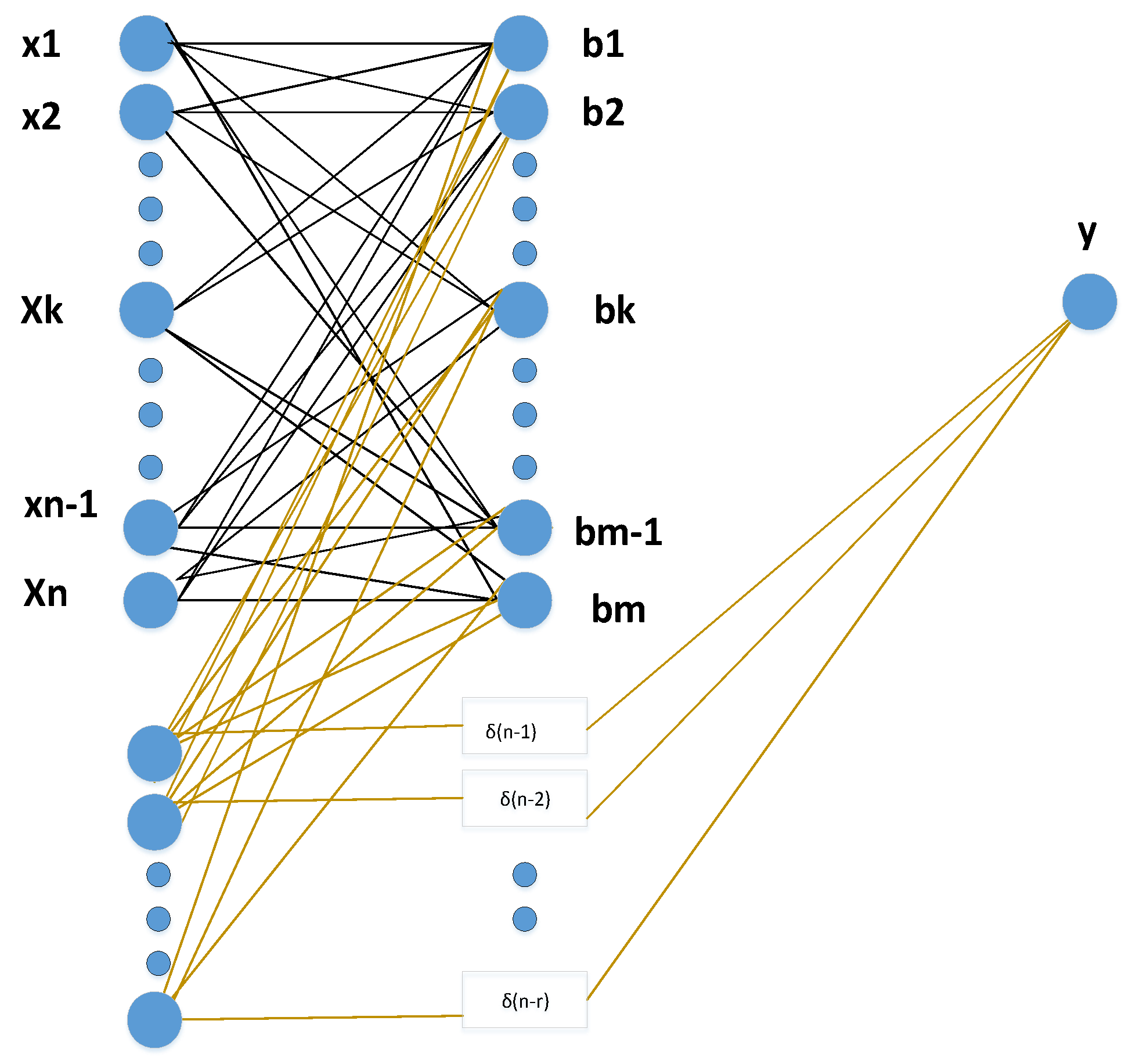
Energies 12 00866 g001
Figure 2. Functioning of RELM.
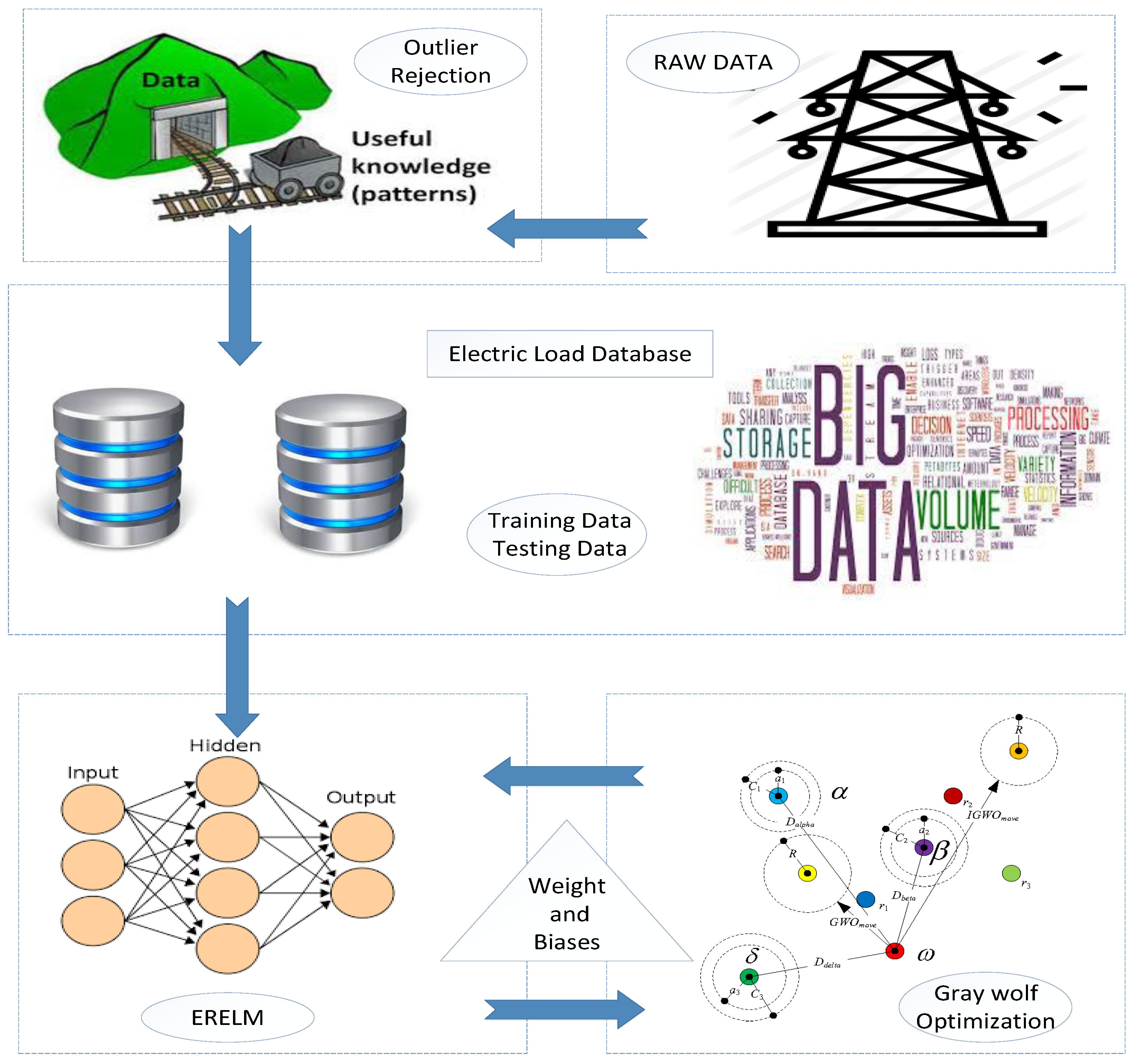
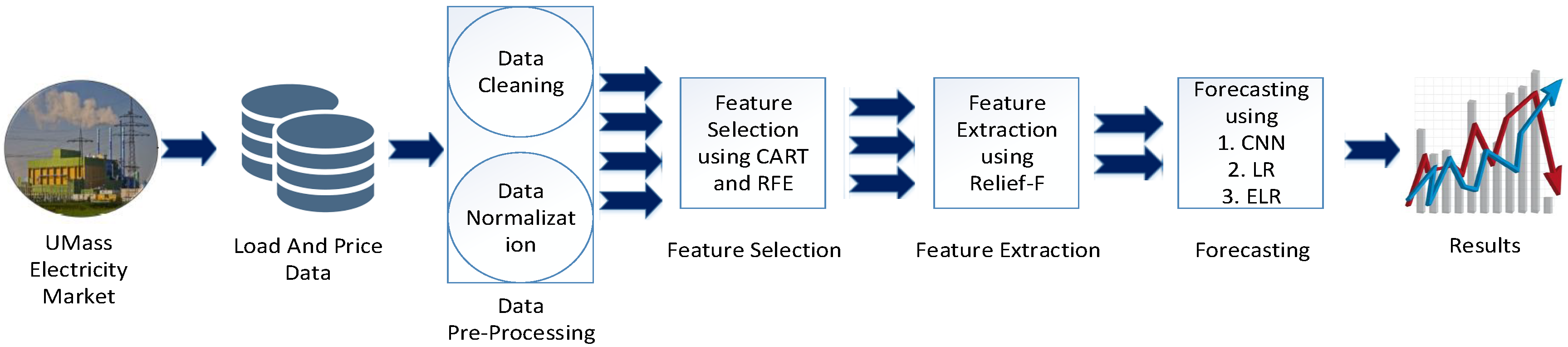
Energies 12 00866 g002
Figure 3. Proposed system model 1.
Energies 12 00866 g003
Figure 4. Proposed system model 2.
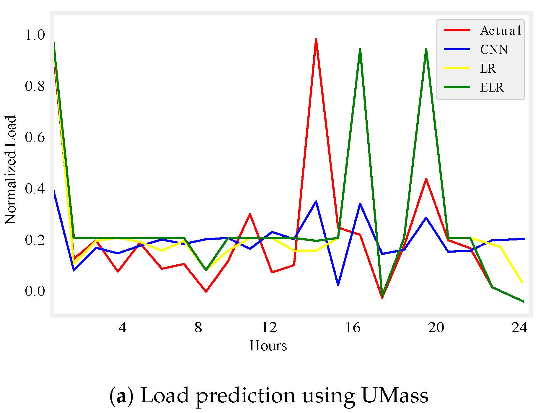
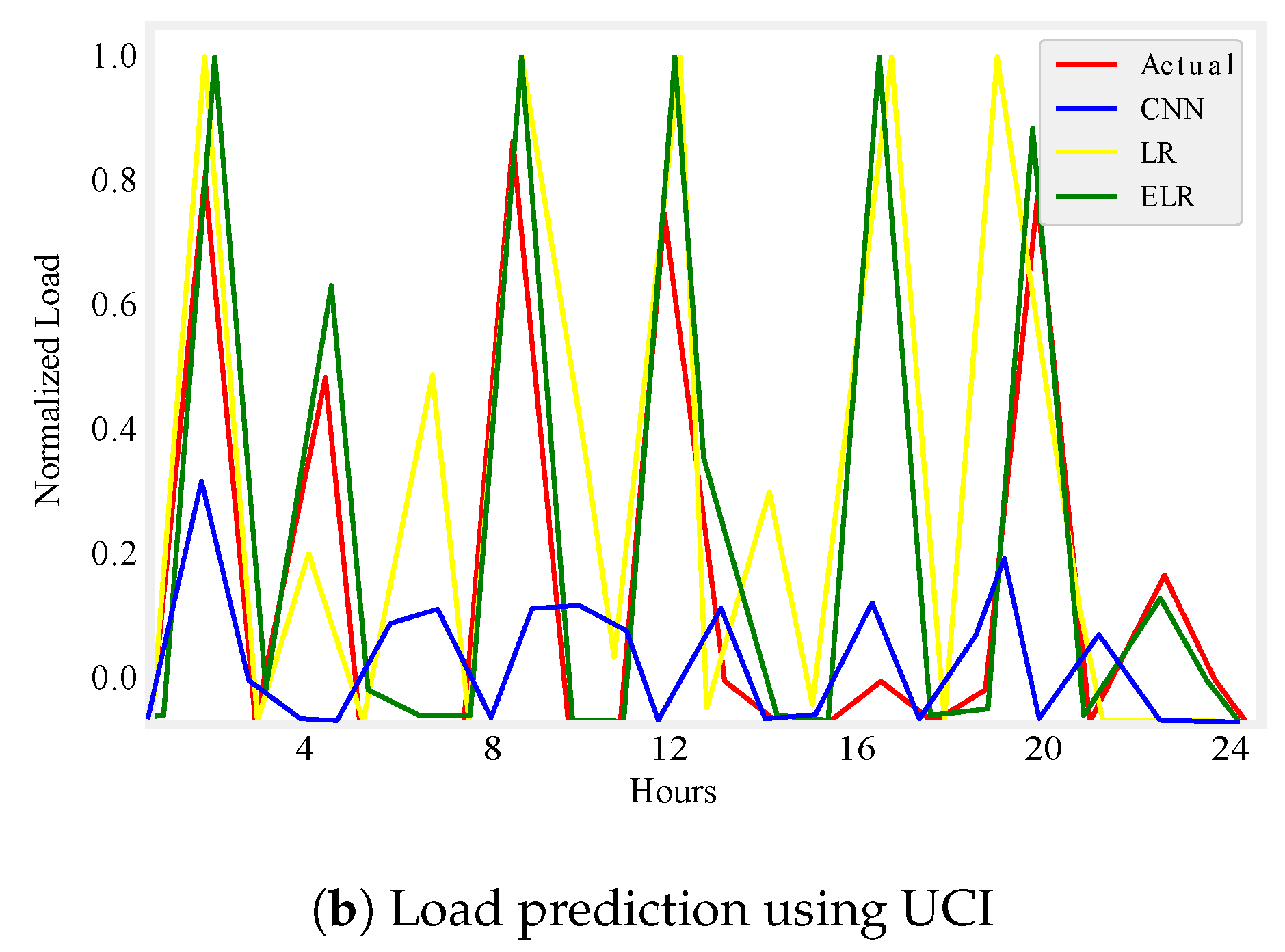
Energies 12 00866 g004
Figure 5. One day load prediction.
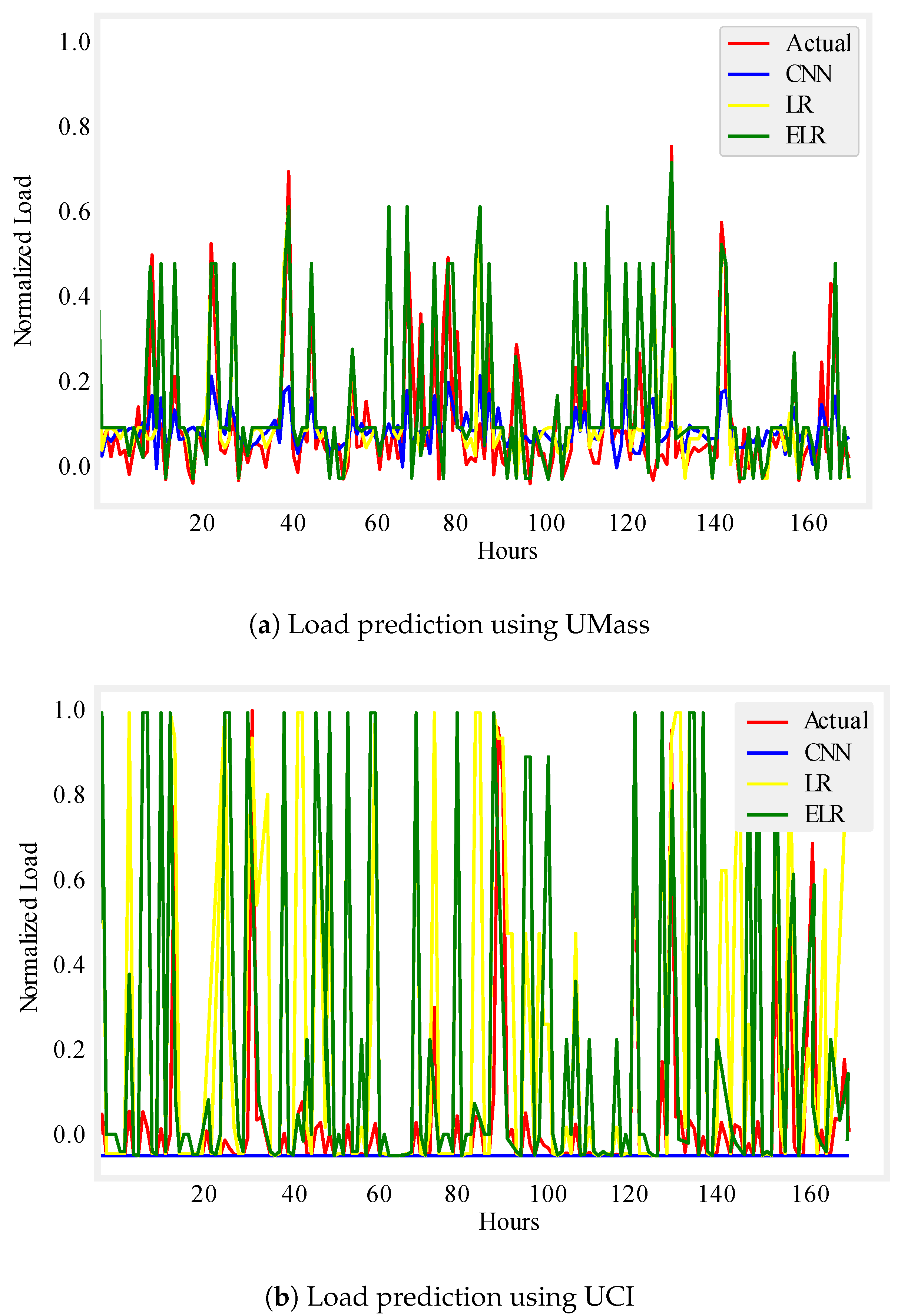
Energies 12 00866 g005aEnergies 12 00866 g005b
Figure 6. One week load prediction.
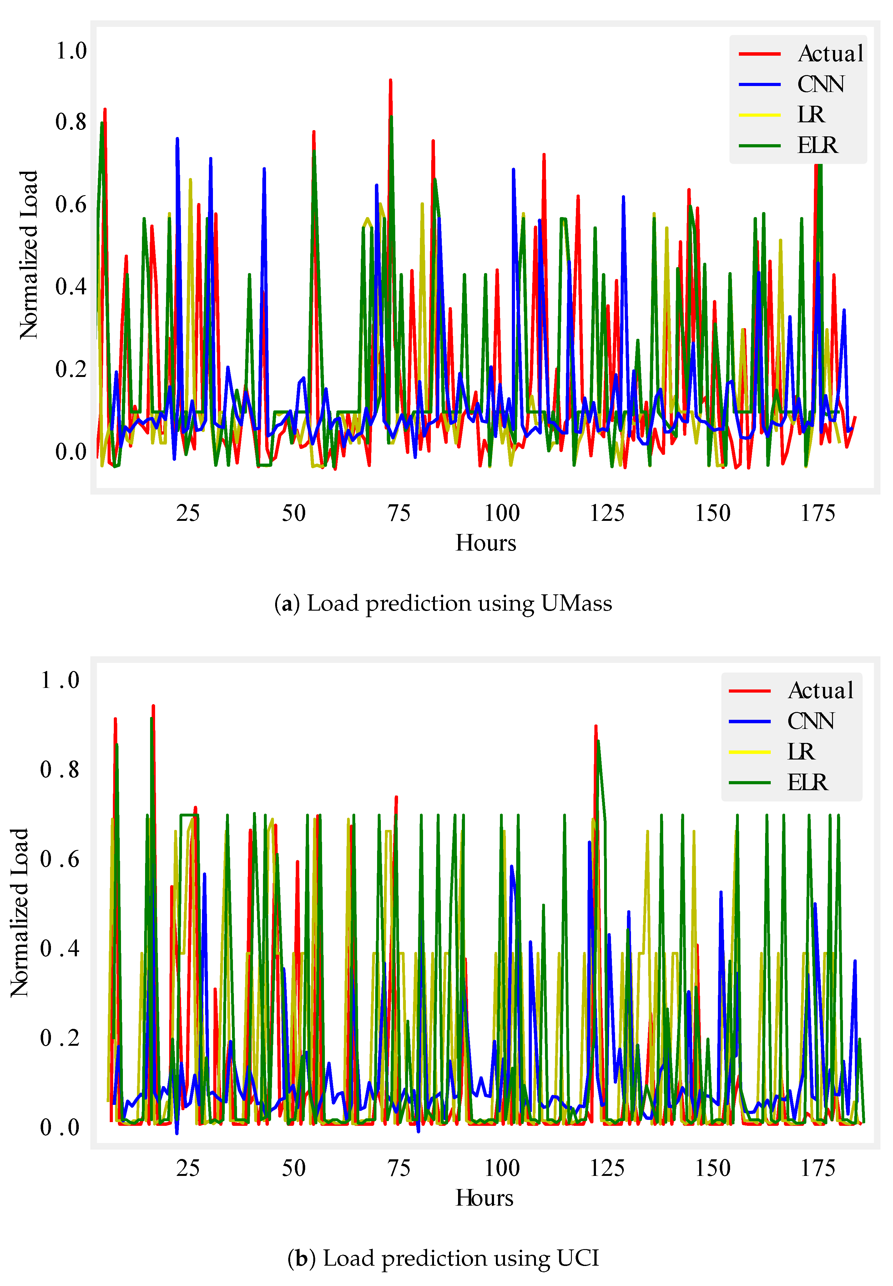
Energies 12 00866 g006
Figure 7. One month load prediction.
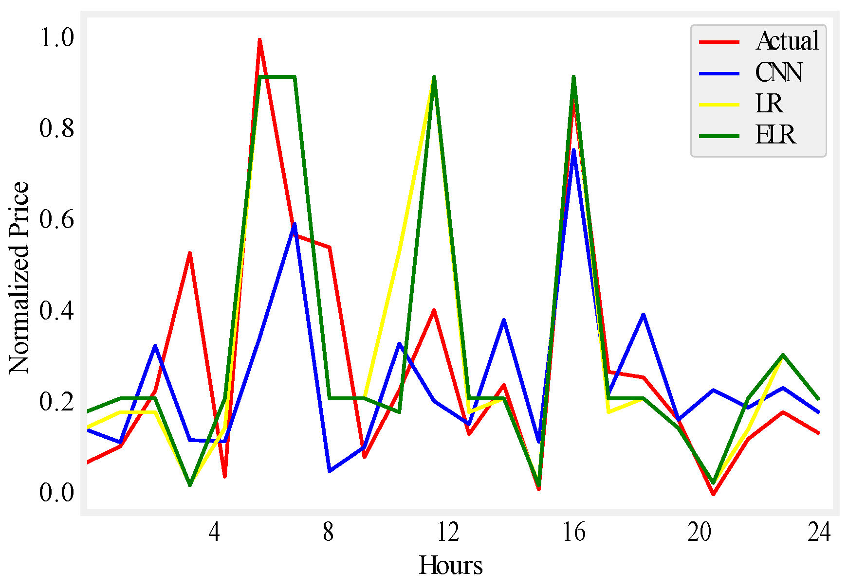
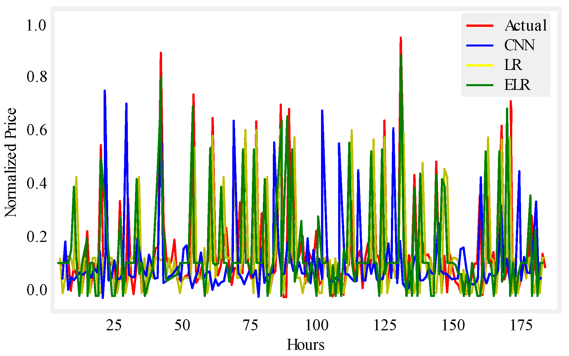
Energies 12 00866 g007
Figure 8. One day price prediction using UMass.
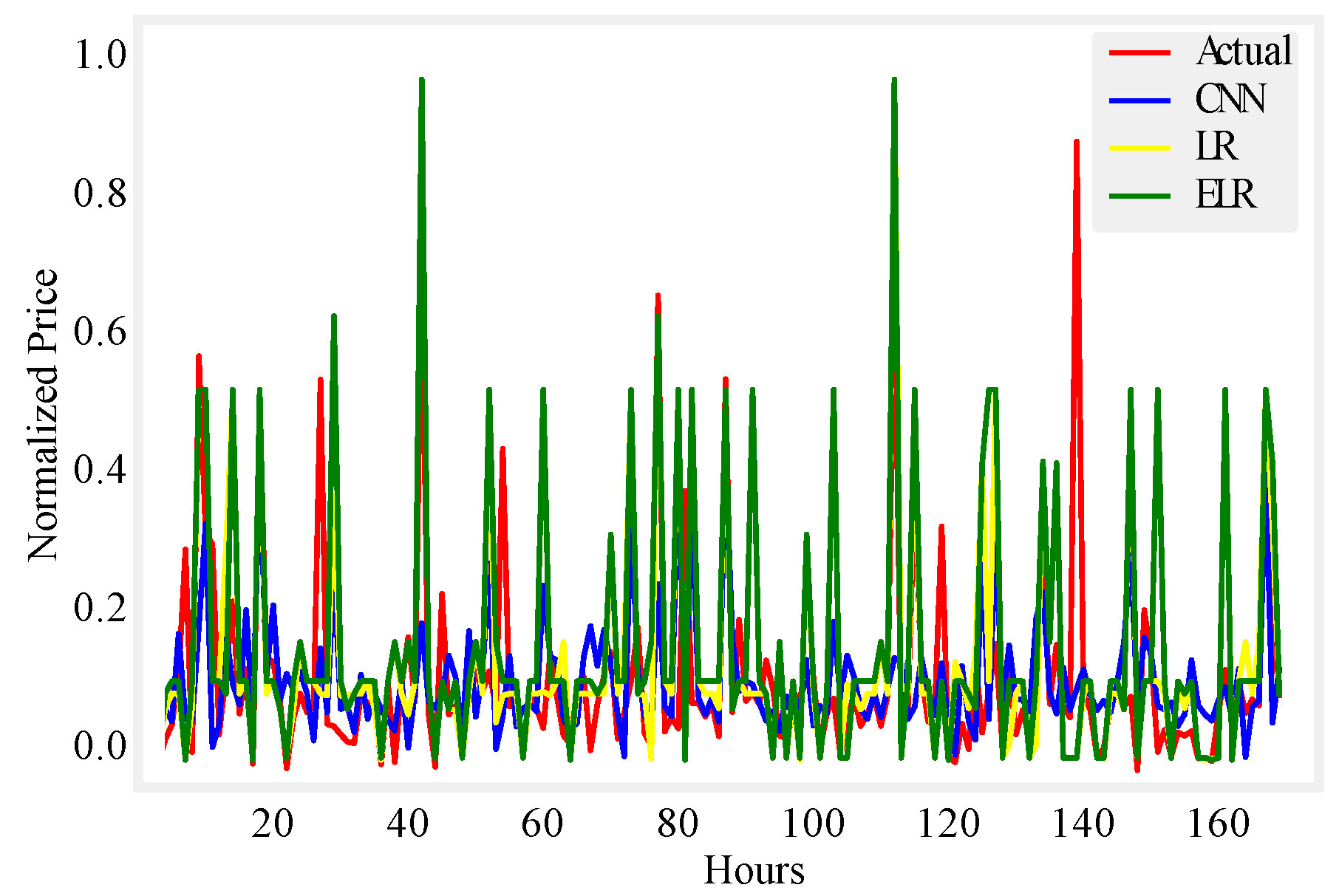
Energies 12 00866 g008
Figure 9. One week price prediction using UMass.
Energies 12 00866 g009
Figure 10. One month price prediction using UMass.
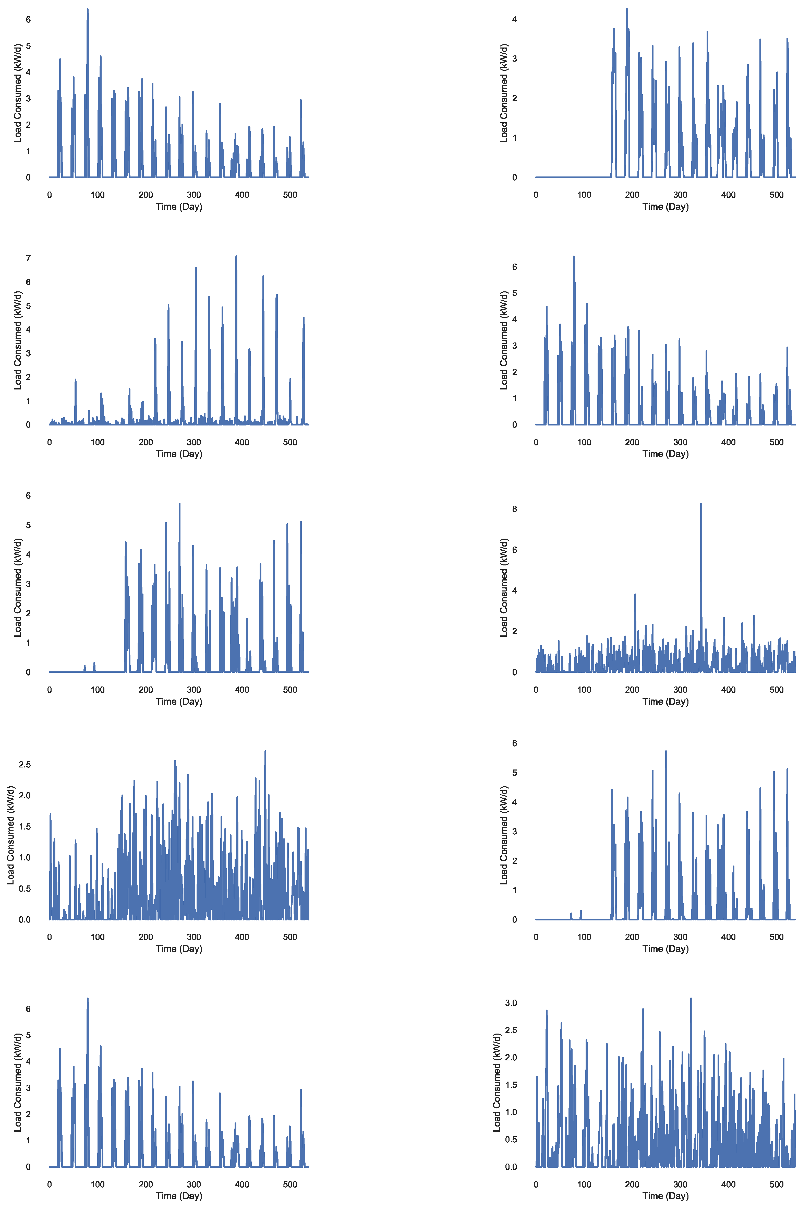
Energies 12 00866 g010
Figure 11. Daily load consumption of 10 different substations.
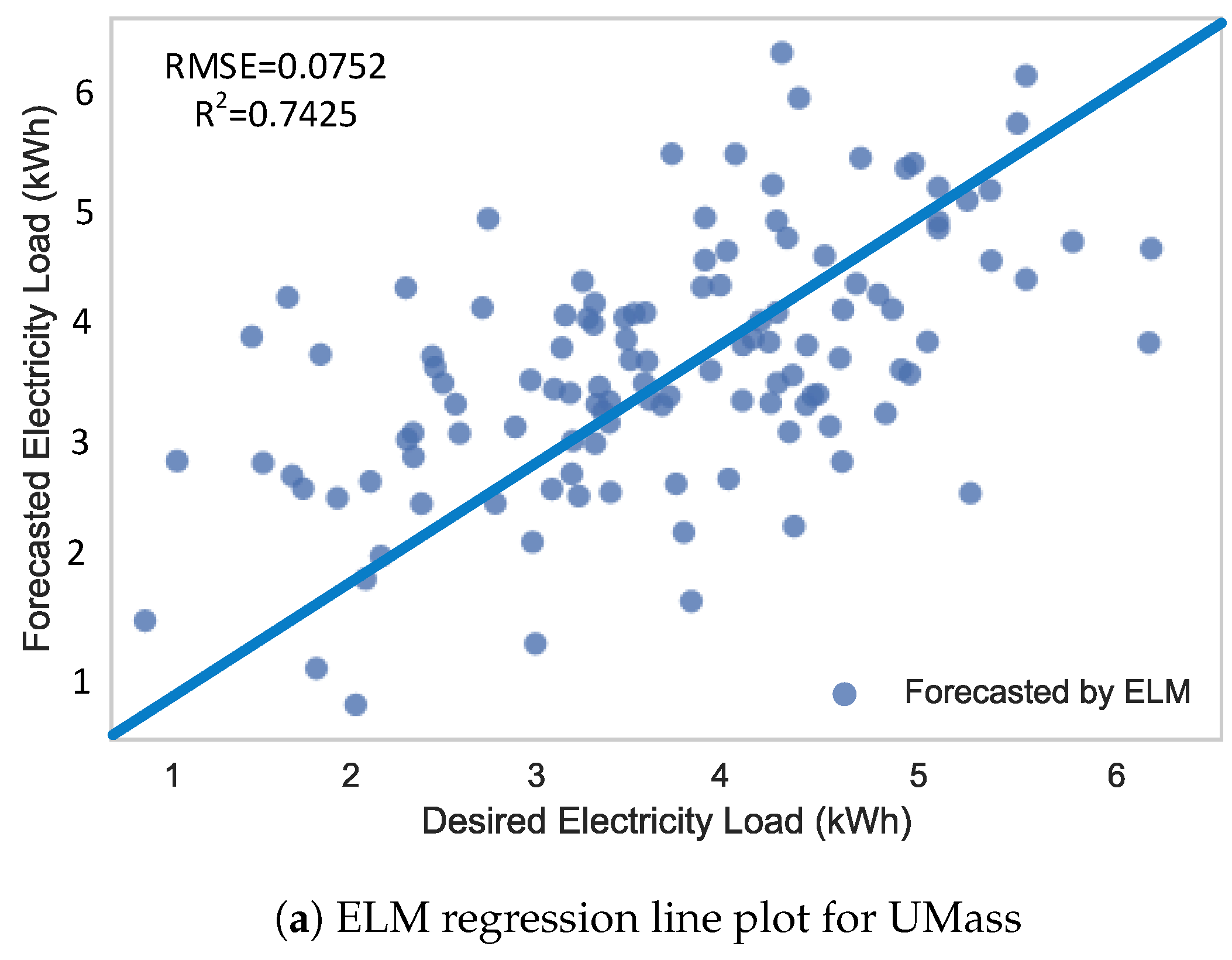
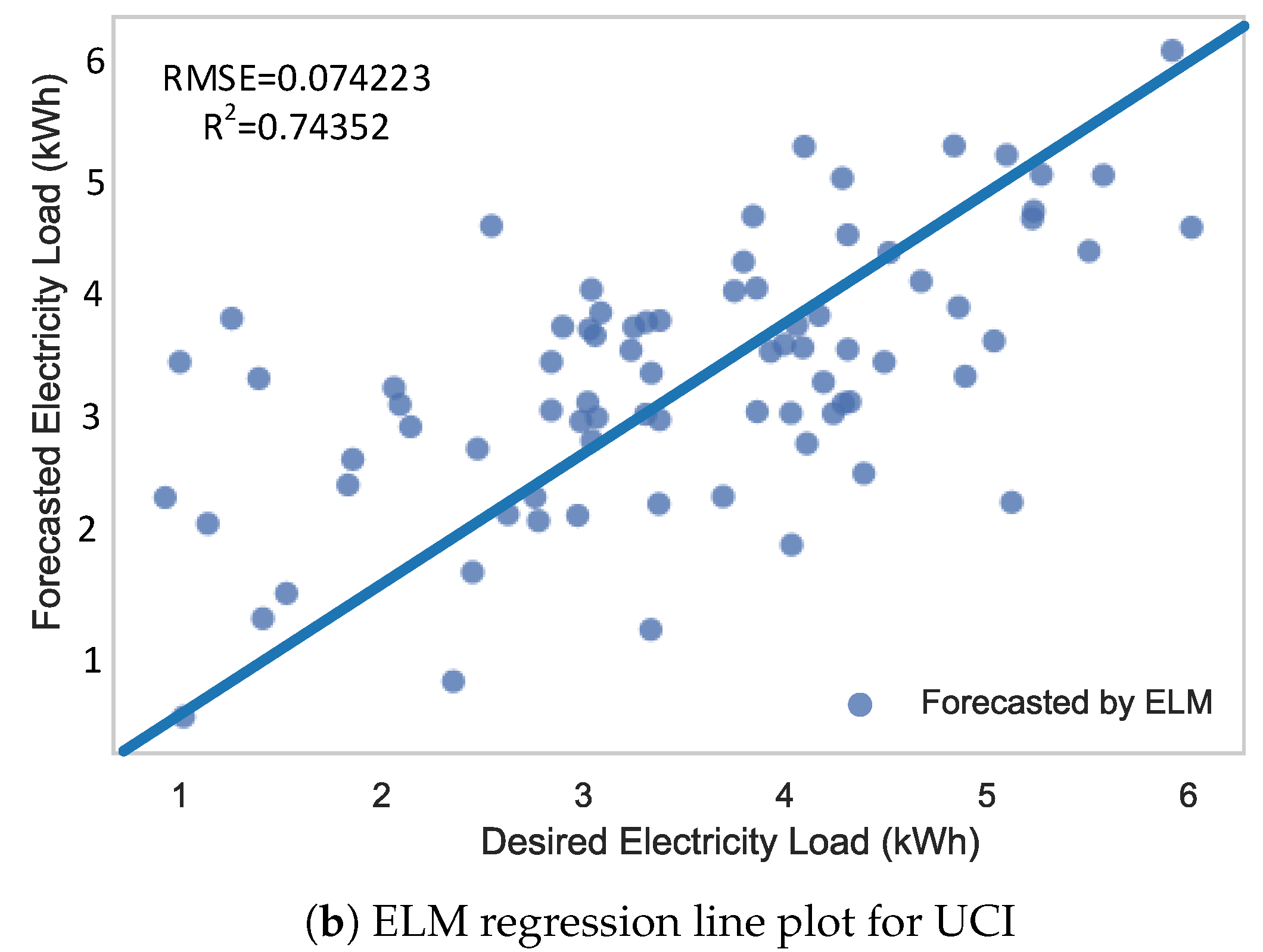
Energies 12 00866 g011
Figure 12. Regression line plots using ELM.
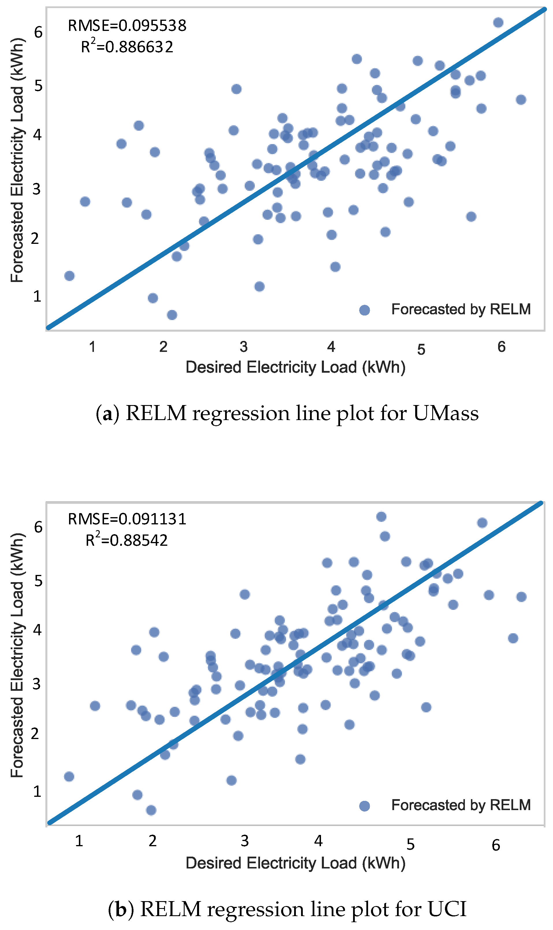
Energies 12 00866 g012aEnergies 12 00866 g012b
Figure 13. Regression line plots using RELM.
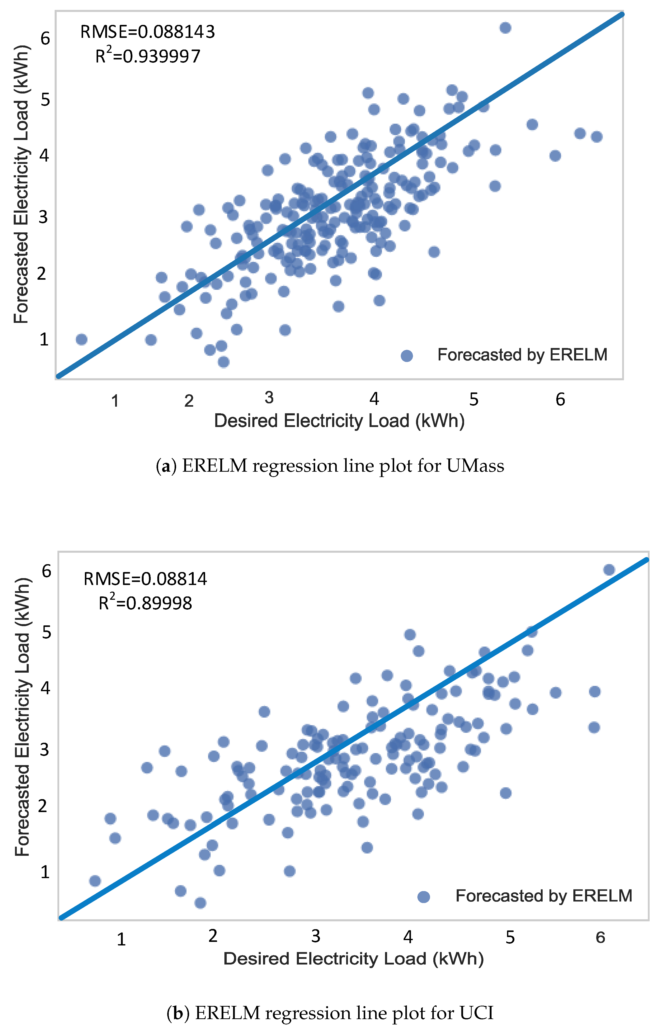
Energies 12 00866 g013
Figure 14. Regression line plots using ERELM.
Energies 12 00866 g014
Table 1. Differences between TG and SG.
TGSG
AnalogueDigital
One way communicationTwo way communication
Centralized power generationDistributed power generation
Small number of sensorsLarge number of sensors
Manual monitoringAutomatic monitoring
Difficult to locate failuresEasy to locate failures
Table 2. List of abbreviations.
AbbreviationFull Form
AEMOAustralia Electricity Market Operators
AIArtificially Intelligent
ANNArtificial Neural Network
ARIMAAuto Regressive Integrated Moving Average
ARMAXAuto Regressive Moving Average with Exogenous variables
BPBack Propagation
CARTClassification and Regression Technique
CNNConvolutional Neural Network
DAEDeep Auto Encoders
DE-SVMDifferential Evolution Support Vector Machine
DNNDeep Neural Network
DRNDeep Residual Network
DSMDemand Side Management
DWTDiscrete Wavelet Transform
ELMExtreme Learning Machine
EPEXEuropean Power Exchange
ELREnhanced Logistic Regression
ERELMEnhanced Recurrent Extreme Learning Machine
FFNNFeed Forward Neural Network
GCAGray Correlation Analysis
GWOGrey Wolf Optimization
GRUGated Recurrent Unit
ISO NECAIndependent System Operator New England Control Area
KELMKernel Extreme Learning Machine
KPCAKernel Principal Component Analysis
LRLogistic Regression
LSTMLong Short Term Memory
MAEMean Absolute Error
MAPEMean Absolute Percentage Error
MISOMidcontinent Independent System Operator
MLPMulti Layer Perceptron
MLRMulti Linear Regression
MSEMean Square Error
NLS-SVMNonlinear Least Square Support Vector Machine
NNNeural Network
NYISONew York Independent System Operator
OS-ELM7Online Sequential Extreme Learning Machine
PJMPennsylvania–New Jersey–Maryland
PSOParticle Swarm Optimization
RBMRestricted Boltzmann Machine
RELMRecurrent Extreme Learning Machne
ReLURectified Linear Unit
RESRenewable Energy Sources
RFERecursive Feature Elimination
RMSERoot Mean Square Error
RNNRecurrent Neural Network
SARIMASeasonal Auto Regressive Integrated Moving Average
SBELMSparse Bayesian Extreme Learning Machine
SDAStacked De-noising Autoencoders
SGSmart Grid
SLFNSingle Layer Feedforward Network
SMSmart Meters
TGTraditional Grid
TVC-ABCTime Varying Coefficients Artificial Bee Colony
Table 3. List of symbols.
SymbolDescription
xActual value
x’Predicted value
tTime slot
yOutput
hStep size
mMean
A v Actual value
F v Forecasted value
TTotal time duration
NTotal number of samples
α Fittest wolf 1
β Fittest wolf 2
δ Fittest wolf 3
ω Remaining wolves
Table 4. Summary of related work.
TechniqueFeatures/DataSetRegionContributionsLimitations
Bayesian, MLP [8]Load/UKDaleUKForecasting done using behavioural analyticRequires intensive training
MLR, BaggedT, NN [9]Load and weather/BeijingBeijing, ChinaComparison between techniques done to overcome the limitationsNot suitable for long term forecasting
DRN [10]Load and weather/ISO-NENew EnglandLoad forecasting done using weather dataOver fitting
RBM, ReLU [11]Load/Korea Electric CompanyKoreaTwo stage forecasting performedLong-term forecasting not supported
DWT-IR, SVM, SWA [12]Load/NYISO, AEMOAustralia, USDimensionality reduction and paramater optimization doneTime complexity
Modified MI, ANN [13]Load/PJMUSTwo stage forecasting is doneTime complexity
DAE [14]Load/Hong KongHong KongCooling load prediction doneTime and space consuming
Pooling Deep RNN [15]Load/IRISHIrelandPooling of consumers done for aggregated predictionDifficult to train
ELM [16,17]Load/USFUSLong, medium and short term forecasting doneOver fitting
SLFN [18,19]Load/Marine Resources DivisionAustraliaOptimization of weightsOverfitting by using moore-penrose inverse
Sparse Bayesian ELM [20]Electricity Load/Harvard medical collegeUSAOptimization of weights and biases using BPRequire intensive training
PSO, DPSO [21]Load/USUSACompact ANNs are producedLarge computational time
GWO with NN [22] USAWeights and biases optimizationTime complexity
RELM [6,23]Electricity Load/Bench mark UCI machinePortugalUse of context neuronsComputationally expensive
LSTM, DNN, GRU [24]Load and price/EPEXBelgiumComparison between different modelsOver fitting
Hilbertian, ARMAX [25]Price/EPEXSpain, GermanyOptimization of functional parameters for price forecastingNon linearity
CNN, LSTM [26]Price/PJMUSTwo NNs are used for price forecastingComputationally expensive
DNN [27]Price/EPEXBelgiumComplex patterns are extracted for predictionSpace complexity
GCA, KPCA, DE-SVM [28]Price/ISO NE-CANew EnglandDimensionality reduction is removed using hybrid of KPCA and GCAOver fitting
SDA [29]Price/MISOArkansas, Texas and IndianaVariant of autoencoder usedComputationally expensive
ARIMA, TVC-ABC, NLS-SVM [30]Price/PJM, NYISO, AEMOAustralia, USParameter tuning of SVM done using TV-ABCComputationally expensive
ANN with meta heuristics optimization methods [31]Load and price/Commercial load of building in China, Taiwan regional electricity loadTaiwanVarious paramater calculations done for accuracyAccuracy of models depend on nature of dataset
OS-ELM with kernel [32]Load and price/Sylva bench markUSComparison of different algorithms doneRestrict to the computation of streamed data
ELM in multi class scenario [33]Load and price/University of California IrvineCanadaRobust classificationComputational cost overhead
Enhanced Logistic RegressionLoad and Price/UMass Electric DatasetUSAELR beats conventional techniquesLarge computational time
RELM enhanced using GWOLoad and Price/UCI DatasetUSAOptimized weights and biases leads to better predictionLarge computational time is required for weight optimization
Table 5. Features in UMass Electric Dataset.
Original Features
Air Conditioner (AC), Furnace, Cellar lights, Washer, First floor lights, Utility room + Basement, Garage outlets, Master bed + Kids bed, Dryer, Panels, Home office, Dining room, Microwave, Fridge
Table 6. Results of CART for UMass Electric Dataset.
FeaturesLoad ValuesPrice Values
AC0.66530.6633
Furnace0.01030.0101
Cellar lights0.00180.0011
Washer0.00290.0029
First floor0.00320.0026
Utility + Basement0.06150.0670
Garage0.00360.0070
M. bed + K. bed0.00800.0059
Dryer0.18900.1927
Panels0.00330.0030
Home office0.08260.0083
Dining room0.00790.0084
Microwave0.02960.0262
Table 7. RFE features for a UMass Electric Dataset.
TypeNumber of Features
Original16
Selected8
Rejected8
Table 8. Relief-F features for UMass Electric Dataset.
ParametersValues
Threshold10
Selected features5
Nearest Neighbors3
Table 9. Obtained RMSE using ELM, RELM and ERELM.
Transfer FunctionForecasting ApproachTrainingTesting
ELM0.05320.0535
Hard LimitRELM0.04120.0423
ERELM0.03320.0345
ELM0.05130.0525
SinRELM0.03520.362
ERELM0.03210.0523
ELM0.06340.0673
TanhRELM0.04530.0463
ERELM0.03410.0321
ELM0.04230.473
SigmoidRELM0.03410.0381
ERELM0.02140.0235
Table 10. Obtained RMSE for half-yearly testing data using ELM, RELM and ERELM by Monte Carlo and K-Fold cross validation.
DatasetsERELMRELMELMRNNLR
Monte CarloK-FoldMonte CarloK-FoldMonte CarloK-FoldMonte CarloK-FoldMonte CarloK-Fold
MT1660.02350.02650.07340.07880.08240.08830.082340.08520.08530.0873
MT1680.01340.01620.04210.04620.05240.04230.08540.08620.07560.0763
MT1690.01530.023520.05310.03530.03820.04630.08530.08730.07350.0762
MT1710.03540.04230.05240.05520.06340.06430.08540.08520.0720.0712
MT1820.02420.03530.02520.03520.08350.09520.07530.07760.09340.0952
MT2350.01530.01420.03440.03970.06340.06430.08650.9340.9810.0991
MT2370.02430.02970.05340.05350.07520.07950.07560.07620.07950.08255
MT2490.01430.01630.05240.05320.06240.06930.08620.08910.07530.0778
MT2500.03420.04520.05350.05620.08530.08730.07640.07840.08740.0894
MT2570.02420.02150.04130.04130.06420.06830.07530.07940.08930.0934
UMass Electric0.03980.03150.05340.05630.06810.06850.07120.08910.08880.0913
Table 11. Obtained RMSE for yearly testing data using ELM, RELM and ERELM by Monte Carlo and K-Fold cross validation.
DatasetsERELMRELMELMRNNLR
Monte CarloK-FoldMonte CarloK-FoldMonte CarloK-FoldMonte CarloK-FoldMonte CarloK-Fold
MT1660.02240.02420.06510.06650.07560.08010.087320.07920.08620.0851
MT1680.01240.01510.06340.07320.05210.04100.08310.07310.07010.0678
MT1690.01440.02240.05010.05530.04240.04310.08120.09120.07410.0872
MT1710.01420.04010.04210.05380.05120.06820.07810.07920.07120.0882
MT1820.01820.02000.02420.02500.07430.07910.08240.07010.08920.0822
MT2350.01420.01520.03010.03620.05820.06020.08520.08920.08890.0986
MT2370.02240.02670.05130.05210.06230.06320.07010.07890.08620.0813
MT2490.01320.01570.04210.06130.05230.06230.07820.08020.06710.0742
MT2500.02420.02730.04120.05010.06020.06920.06820.07720.07850.0864
MT2570.03240.04720.04010.05130.06020.07440.06230.07020.08760.0882
UMass Electric0.03320.04120.05420.05520.05820.06030.07010.07710.08210.0891
Table 12. Computational time comparison of ERELM, RELM and ELM execution.
Forecasting TechniqueTraining Time (s)Testing Time (s)
ERELM0.6530.0346
RELM0.00430.0012
ELM0.001240.001076
Table 13. Load performance metrics comparison for one day using the UMass Electric Dataset.
MetricsHalf-Yearly DataYearly Data
CNNLRELRCNNLRELR
MSE (abs. val)8.845.844.7710.28.976.8
MAE (abs. val)9.245.254.348.756.254.24
RMSE (abs. val)10.627.646.1810.46.65.2
MAPE (%)25.4422.4518.4836.333.330.5
Accuracy (%)89.3892.3593.8289.693.494.8
Table 14. Load performance metrics comparison for one week using the UMass Electric Dataset.
MetricsHalf-Yearly DataYearly Data
CNNLRELRCNNLRELR
MSE (abs. val)20.217.9712.9718.916.511.3
MAE (abs. val)8.826.875.288.756.255.19
RMSE (abs. val)16.2513.1210.1815.7612.989.64
MAPE (%)25.6522.1917.4133.225.922.8
Accuracy (%)83.7586.8889.8184.2487.0291.36
Table 15. Load performance metrics comparison for one month using the UMass Electric Dataset.
MetricsHalf-Yearly DataYearly Data
CNNLRELRCNNLRELR
MSE (abs. val)25.8221.8217.3724.0220.5614.25
MAE (abs. val)10.558.236.7910.358.155.33
RMSE (abs. val)17.8514.7711.7912.559.986.52
MAPE (%)29.1327.1323.3925.4521.220.6
Accuracy (%)82.1585.7288.2187.4590.0293.48
Table 16. Price performance metrics comparison for one day using the UMass Electric Dataset.
MetricsHalf-Yearly DataYearly Data
CNNLRELRCNNLRELR
MSE (abs. val)15.0814.3910.0912.5810.858.6
MAE (abs. val)8.257.656.017.857.055.88
RMSE (abs. val)16.6314.9912.9815.0511.529.85
MAPE (%)19.0218.5917.1120.0518.8515.55
Accuracy (%)83.3785.0187.0284.9588.4890.15
Table 17. Price performance metrics comparison for one week using the UMass Electric Dataset.
MetricsHalf-Yearly DataYearly Data
CNNLRELRCNNLRELR
MSE (abs. val)14.0512.8011.2215.0213.4511.25
MAE (abs. val)7.556.045.038.027.055.25
RMSE (abs. val)13.0511.309.4712.5510.458.64
MAPE (%)14.2513.7113.0316.4515.7515.25
Accuracy (%)86.9588.7090.5387.4589.5591.36
Table 18. Price performance metrics comparison for one month using the UMass Electric Dataset.
MetricsHalf-Yearly DataYearly Data
CNNLRELRCNNLRELR
MSE (abs. val)19.4518.9116.4720.0518.5413.35
MAE (abs. val)8.957.706.449.358.156.42
RMSE (abs. val)14.7813.7511.4812.4411.029.45
MAPE (%)21.4420.5418.8923.3622.5519.45
Accuracy (%)85.2286.2588.5287.5688.9890.55
Table 19. Load performance metrics comparison for one day using the UCI Dataset.
MetricsHalf-Yearly DataYearly Data
CNNLRELRCNNLRELR
MSE (abs. val)15.0512.4710.5618.2014.310.4
MAE (abs. val)12.4510.348.5621.4718.3716.61
RMSE (abs. val)18.5215.5413.4516.2213.7810.16
MAPE (%)28.2425.3420.4527.0523.2520.05
Accuracy (%)81.4884.4686.5583.7886.2289.84
Table 20. Load performance metrics comparison for one week using the UCI Dataset.
MetricsHalf-Yearly DataYearly Data
CNNLRELRCNNLRELR
MSE (abs. val)25.2019.6615.7713.258.347.2
MAE (abs. val)11.3510.018.2413.9812.4711.39
RMSE (abs. val)22.4519.2516.4520.2517.8013.11
MAPE (%)28.5625.4519.6330.5025.4518.52
Accuracy (%)77.5580.7583.5579.7582.2086.89
Table 21. Load performance metrics comparison for one month using the UCI Dataset.
MetricsHalf-Yearly DataYearly Data
CNNLRELRCNNLRELR
MSE (abs. val)28.3525.5521.6815.5013.85.47
MAE (abs. val)15.3510.348.9523.4619.317.7
RMSE (abs. val)23.9720.8717.6920.0217.1714.49
MAPE (%)31.2329.4325.6727.4525.3520.02
Accuracy (%)76.0379.1382.3179.9882.2385.51
Table 22. Accuracy of ERELM using RMSE, MSE and MAE for half-yearly data.
DatasetsRMSEMSEMAE
MT1660.02350.000550.0243
MT1680.01340.000170.0135
MT1690.01530.000230.0174
MT1710.03540.001250.0352
MT1820.02420.000580.0252
MT2350.01530.000230.0253
MT2370.02430.000590.0254
MT2490.01430.000200.0153
MT2500.03420.0011690.0342
MT2570.02420.000580.0253
UMass Electric0.02560.000710.0623
Arithmetic Mean0.02270.000550.024218
Standard Deviation0.006000.0003500.006515
Table 23. Accuracy of ERELM using RMSE, MSE and MAE for yearly data.
DatasetsRMSEMSEMAE
MT1660.02240.000410.0215
MT1680.01240.000160.0142
MT1690.01440.000150.0162
MT1710.01420.001240.0221
MT1820.02000.000420.0224
MT2350.01420.000470.0201
MT2370.02240.000150.0241
MT2490.01320.000120.0142
MT2500.02420.001020.0163
MT2570.03240.000450.0177
UMass Electric0.03320.000610.0546
Arithmetic Mean0.020270.000470.02212
Standard Deviation0.007120.000340.01077

