Two-Stage Stochastic Optimization for the Strategic Bidding of a Generation Company Considering Wind Power Uncertainty

Abstract

With the deregulation of electricity market, generation companies must take part in strategic bidding by offering its bidding quantity and bidding price in a day-ahead electricity wholesale market to sell their electricity. This paper studies the strategic bidding of a generation company with thermal power units and wind farms. This company is assumed to be a price-maker, which indicates that its installed capacity is high enough to affect the market-clearing price in the electricity wholesale market. The relationship between the bidding quantity of the generation company and market-clearing price is then studied. The uncertainty of wind power is considered and modeled through a set of discrete scenarios. A scenario-based two-stage stochastic bidding model is then provided. In the first stage, the decision-maker determines the bidding quantity in each time period. In the second stage, the decision-maker optimizes the unit commitment in each wind power scenario based on the bidding quantity in the first stage. The proposed two-stage stochastic optimization model is an NP-hard problem with high dimensions. To tackle the problem of “curses-of-dimensionality” caused by the coupling scenarios and improve the computation efficiency, a modified Benders decomposition algorithm is used to solve the model. The computational results show the following: (1) When wind power uncertainty is considered, generation companies prefer higher bidding quantities since the loss of wind power curtailment is much higher than the cost of additional power purchases in the current policy environment. (2) The wind power volatility has a strong negative effect on generation companies. The higher the power volatility is, the lower the profits, the bidding quantities, and the wind power curtailment of generation companies are. (3) The thermal power units play an important role in dealing with the wind power uncertainty in the strategic bidding problem, by shaving peak and filling valley probabilistic scheduling.

1. Introduction

1.1. Background and Motivations

During the last several decades, the electricity industry all over the world was long dominated by vertically integrated utilities. In order to improve the energy efficiency and social welfare, as well as reduce the operational cost of the electricity industry, many countries are struggling to reform their electricity sectors. The electricity markets throughout the world are now undergoing huge restructuring processes. In a liberalized electricity market, the electricity market in each time period is formed through an auction mechanism, which is called day-ahead power exchange. Using this mechanism, an independent system operator matches the sellers’ and buyers’ bids to determine the market clearing price corresponding to the equilibrium point of electricity market. Under this context, it is of great significance for generation companies to optimize its bidding decisions in order to earn more profit.

In line with the above government consideration, researchers are intensively studying strategic bidding. Previously, some traditional energy sources represented by fossil fuels play a dominant role in the power structure of most countries. Therefore, most previous literature with regard to strategic bidding focuses on the thermal power generation companies. However, it is known to all that fossil fuels are limited and unrenewable. Its overconsumption may also bring several environmental pollution problems. With the increasing concern over the energy security and environmental pollution caused by the overconsumption of fossil fuel, the development of renewable energy sources such as wind power will be a prevailing trend. The integration of renewable power sources is expected to constantly rise. Take China as an example. By 2017, China ranked first in the global ranking of new installed wind power capacity, with a total installed wind power capacity of 19,660 MW, accounting for 37% of the market share, and the installed wind power capacity of China will exceed 2 × 10³ GW in 2018, which will be a milestone in the history of wind power development in China [1]. In response to the rapid development of wind power generation, this paper will focus on the strategic bidding of a generation company with wind farms.

When considering the strategic bidding of a generation company with wind farms, one of the most important problems that must be solved is wind power uncertainty. It is worth noting that, although the integration of wind power has brought considerable environmental benefits, it has also posed great challenges to the reliability and economic of electric power systems due to its intermittent and stochastic nature. Since the exact value of wind power output in each time period is unknown, it may confuse the decision-makers when they offer their bidding quantities in the day-ahead electricity market. As a powerful tool in dealing with the uncertainty, stochastic programming theory has been widely used in electric power systems to handle the uncertain parameters. In this paper, we use two-stage stochastic optimization theory to handle wind power uncertainty.

1.2. Aims and Contributions

This paper provides a two-stage stochastic optimization model for the strategic bidding of a generation company with both thermal power units and wind farms. Note that the decisions of the strategic bidding of a generation company usually involve two processes: (1) a bidding process and (2) a production process. In the former, a generation company offers its bidding quantity and bidding price in a day-ahead electricity market. After the bidding process ends, the generation company optimizes the production schedule of electricity to satisfy the bidding quantity the next day. We divide the decision variables of a generation company into two categories: first-stage and second-stage. We assume that bidding quantity is a first-stage variable. Since the decision-maker must offer its bidding quantity in a day-ahead electricity market, the exact value of wind power is unknown. We assume that wind power uncertainty disappears the next day. The decision-maker then optimizes the production schedule of electricity based on the first-stage variable and the exact value of wind power. The proposed model is an NP-hard problem with high dimensions. If we solve it directly through branch and bound algorithms, the problem of “curses-of-dimensionality” caused by the coupling scenarios can lead to a heavy computation burden. Based on this consideration, a modified Benders decomposition algorithm is used to solve this model. The innovations of this paper can be shown as follows:

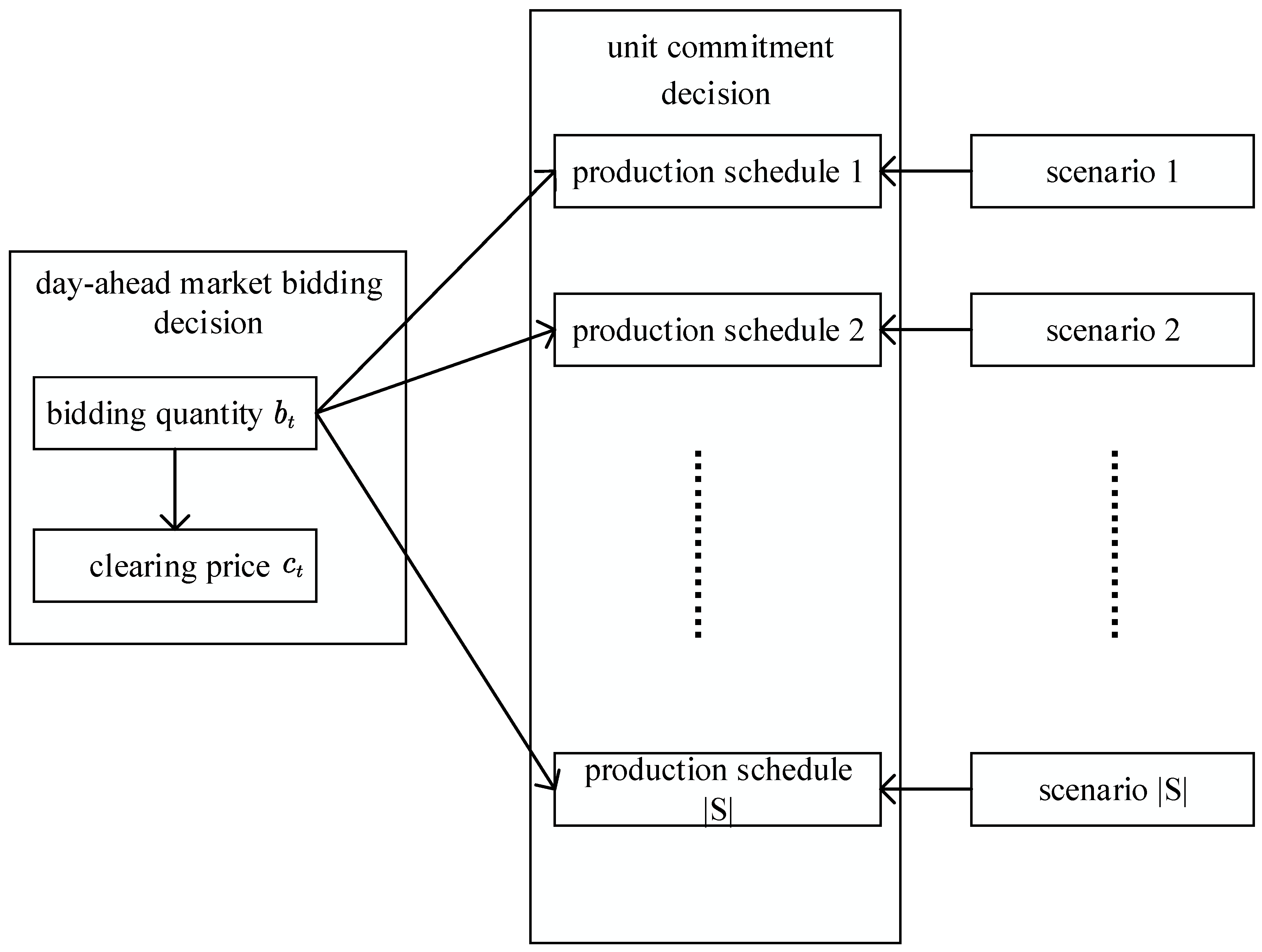
• Based on the two-stage stochastic optimization theory, the decision-making of power generation enterprises is divided into a day-ahead bidding decision and a real-time scheduling decision according to the different decision-making stages. A two-stage stochastic optimization model is constructed.
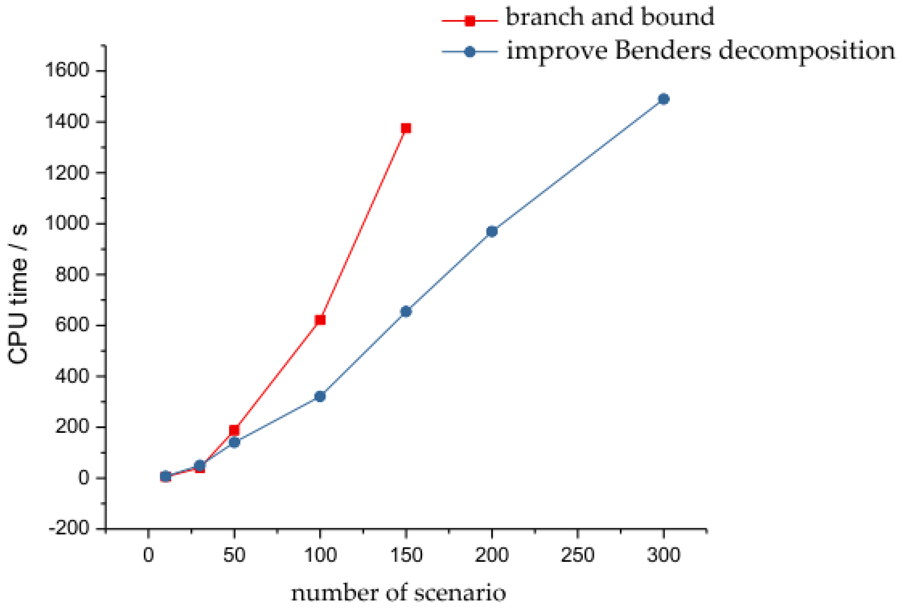
• An improved Benders decomposition algorithm is used to solve the problem. This algorithm decomposes the original problem into a master problem that only involves first-stage variables, and a set of sub-problems that only involves second-stage variable. These problems are much easier to solve compared with the original problem. This modified Benders decomposition algorithm does not requires the sub-problem to be a convex optimization problem like the traditional Benders decomposition algorithm. Note that the sub-problems in this paper are mixed integer programming since the startup and shutdown decisions of thermal power units are involved. We use a convex hull approximation method to convexify the feasible region of the sub-problem, so that the dual information of the sub-problem can be utilized.
• The actual cases from the Latin American electricity market are selected to verify the rationality and effectiveness of the constructed models and algorithms.

1.3. Paper Organization

The content of the paper is arranged as follows: Section 2 reviews the research status of strategic bidding of generation companies and the probabilistic scheduling of wind generators. Section 3 expounds the profit function of power generation enterprises in the free competitive power wholesale market. In Section 4, aiming at maximizing the profit expectation of power generation enterprises, a two-stage stochastic optimization model is established. The algorithm of the mixed integer linear programming model is proposed in Section 5. Using the method proposed in this paper, the actual cases are selected for analysis and discussion in Section 6, and Section 7 summarizes the conclusions of the study.

2. Literature Review

In order to adapt to this trend, many scholars have begun to pay attention to the research on strategic bidding of power generation companies in the deregulated market environment. There are two streams of literature that are closely related to our paper: one is about the strategic bidding of a generation company as a price taker; the other is the probabilistic scheduling of wind generators.

2.1. Strategic Bidding of Generation Company

In terms of strategic bidding of a generation company as a price taker, Ahmet D. Yucekaya [2] et al. considered power operating constraints and price uncertainty within the market to establish bidding models, and two particle swarm optimization algorithms are proposed to determine bidding price and bidding scalar in a competitive power market. Ettore Bompard [3] et al. established a strategic bidding model in oligopoly electricity markets and introduced a demand elasticity model used for assessing the mitigation effects on the strategic bidding of the producers. Based on the strategic bidding problem and Nash equilibrium (NE) concepts, Luiz Augusto Barroso [4] et al. used Nash equilibrium theory to discuss the calculation method of the electricity market-clearing price under the oligopolistic competition market, and discussed the optimal bidding strategy of generation companies based on this clearing price. Li [5] et al. established the bidding strategy model in terms of supply function equilibrium. John W. [6] et al. proposed a framework in which strategies of generating companies may be developed for the individual participants in an energy brokerage, and obtained an optimal bidding strategy. Mario Veiga Pereira [7] et al. considered the strategic bidding problem under the uncertainty of a short-term power market environment, established pure price, pure quantity, or joint price/quantity bidding models, and proposed a binary expansion (BE) solution approach to solve the above problem. Meanwhile, some scholars have studied the bidding of power generation companies in the future free competitive market environment. Kazemi M et al. [8] considered the uncertainty of clearing price in the power market and built an uncertain bidding model for thermal power generators based on information gap decision theory. Ren et al. [9] discussed the optimal bidding strategy for thermal power producers under the dynamic bidding game mode of incomplete information. Considering the real time wind power uncertainties, the pre-bidding model under different bidding strategies was proposed [10]. Ding et al. [11] studied the bidding problem of wind power generators with energy storage systems, and verified the role of energy storage systems in bidding for power generation enterprises. Agustín et al. [12], based on the conditional risk value (CVAR) theory, studied the bidding optimization problem of generation companies with two types of power generation methods: wind power generation and hydropower generation.

2.2. Probabilistic Scheduling of Wind Generators

With regard to probabilistic scheduling of wind generators, many scholars have conducted in-depth research from different angles. Yan et al. [13] classified the uncertainty analysis methods from different perspectives, and summarized and evaluated the commonly used optimization algorithms and future development trend, but did not compare the accuracy of various algorithms quantitatively. Li et al. [14] considered the uncertainty of wind power under the day-ahead market environment, and established a clearing model based on the day-ahead market, which effectively solves the problem of power system scheduling. Zhang et al. [15] established a probabilistic optimization model based on user demand, wind power, and the uncertainty of carbon trading. Aiming at minimizing the total cost of power generation in the system, Bin et al. [16] introduced the scene method into the wind power grid-connected system to establish an optimization model with the goal of minimizing expected cost. Jiang et al. [17] separated wind power into three scenarios, and chose the Benders decomposition method to solve the wind and hydro coordinated optimization model. Fu et al. [18] proposed an operational method to satisfy the fluctuation of wind power in the range, and established a robust optimization economic scheduling model. Álvaro Lorca et al. [19] used a combination of adaptive theory and robust optimization to establish an economic dispatch model to automatically adjust system parameters when wind power changes. Sun et al. [20] proposed a multi-time scale intra-day ultra-short-term scheduling strategy combining intra-day rolling optimization and real-time optimization. Tan et al. [21] used the concepts of demand response and energy storage system to establish a scheduling optimization model of grid-connected wind power. Zhao et al. [22] proposed the expectation and opportunity constraint feathering method for solving random unit combinations. Liu et al. [23] and Guan et al. [24] pointed out various types of uncertain sets and solved the problem of wind power uncertainty. Hu [25] et al. used interval numbers to solve the uncertainty problem of wind power and load. Compared with the traditional method, the proposed method has improved the robustness and economy of the scheduling plan. Suresh K. Damodaran [26] et al. presented the modeling of hydro-thermal-wind generation scheduling considering economic and emission factors, and proposed a modified particle swarm optimization (MPSO) algorithm to solve it.

3. Generation Company Return Function

3.1. Problem Description

Generation companies are no different from other companies whose objective is to make profits. Therefore, it is important to discuss the return function of power generation companies. The return function of selling the electricity during time period $t$ is shown as follows:

$$R_t\left(b_t,c_t\right)=b_t{c}_t$$

(1)

where $b_t$ is the bidding quantity during time period t. $c_t$ is the market clearing price of the electricity wholesale market during the time period $t$. One of the important differences between a deregulated electricity market wholesale market and a traditional highly regulated power wholesale market is the formation mechanism of electricity prices. In a deregulated wholesale electricity market, electricity prices are not determined by national energy policies but are based on market supply and demand. Based on the market clearing rules, the independent system operators of the wholesale electricity market will find an equilibrium point in each time period according to the bidding quantity and quotation provided by the power purchasers and power sellers. The electricity price corresponding to the equilibrium point is called “market clearing price,” which is the unit return of electricity sellers and the unit cost of electricity buyers. Note that different power supply and demand may correspond to different equilibrium points, leading to a different market-clearing price. At present, electricity sellers in the wholesale electricity market fall into two categories, the price maker and the price taker. For price takers, since their installed capacities and bidding quantities are not large, the changes in their bidding quantity are not substantial enough to significantly affect the balance between supply and demand in the market. There is no significant relationship between $b_t$ and $c_t$. $c_t$ can be regarded as a given parameter for the price taker. However, for price makers, the change in the bidding quantity may result in changes in market clearing prices due to their high installed capacities. Therefore, we need to discuss the relationship between $b_t$ and $c_t$ when power generation companies are price makers.

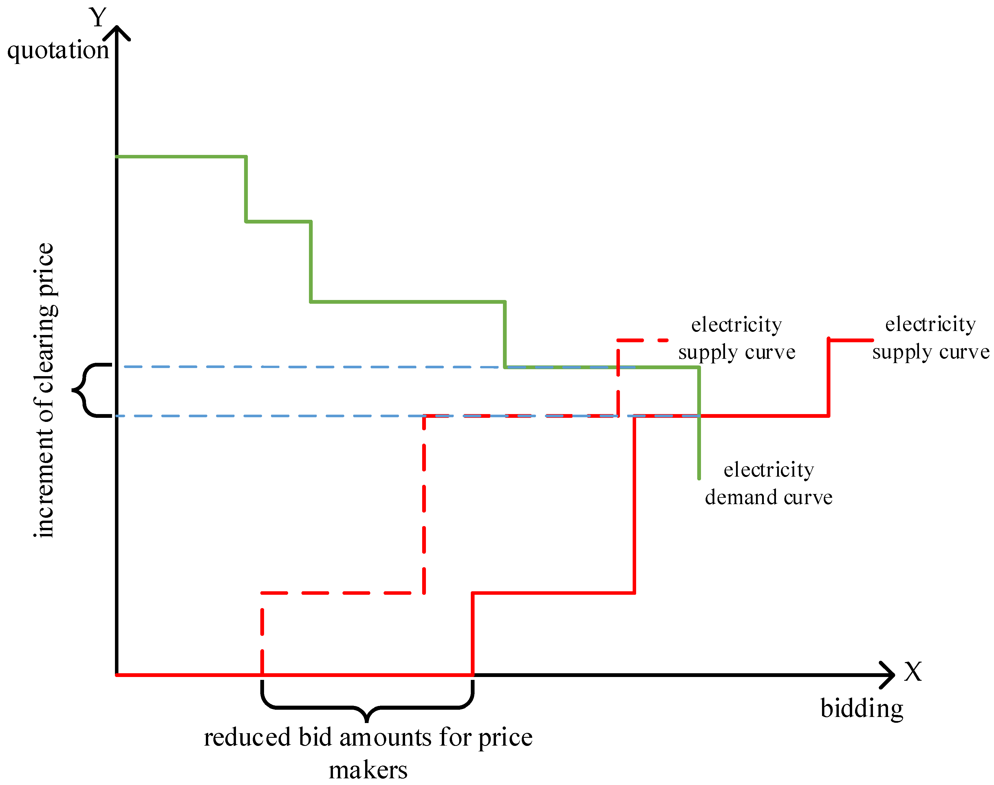
3.2. Electricity Wholesale Supply and Demand Relationship

Considering an electricity wholesale market with one price maker and multiple price takers, this paper focus on the decision-makings of the price maker. The following assumptions are made:

(1)

The relevant information in the wholesale electricity market is completely transparent to the price maker. In other words, the uncertainty of the market information is not considered.

(2)

The bidding prices of the price maker are assumed to be 0 during the entire planning horizon. This ensures that all bidding quantities of the price maker will be sold in the market. This is because the market clearing price in each time period must be greater than 0.

Figure 1 provides the supply and demand in an electricity wholesale market. We use Figure 1 to illustrate how the market clearing price is formed. The green curve and red curve represent the demand of electricity buyers and the supply of electricity sellers, respectively, as well as their bidding prices. The electricity price corresponding to the intersection point between these two curves is the so-called market clearing price. This intersection point is called the equilibrium point in the electricity market. This is because the supply and demand at this point is equal.

Figure 1 also shows how the market clearing price changes with the change in the bidding quantity of a price maker. After the price maker reduces its bidding quantity, the equilibrium point changes from X to Y. Note that X and Y correspond to different market clearing prices, which means that the reduction of the bidding quantity may break the equilibrium state, thus increasing the market clearing price.

The corresponding market clearing price under different bidding quantity can be obtained by changing the length of the step corresponding to the price maker, then observing the electricity price corresponding to the new equilibrium point. The function diagram of a price maker can then be shown as follows:

Let $e_{1t},e_{2t},e_{3t}$ be the break points. If the bidding quantity of a price maker exceeds a break point, the equilibrium state will be broken, which will affect the market-clearing price. $p_{1t},p_{2t},p_{3t}$ are the corresponding market clearing prices under different bidding intervals, which is the slope corresponding to the return function diagram under this interval. Note that, in the bidding interval corresponding to the red image, we can see the case that the bidding amount is higher than the previous break point but the revenue is lower. In this case, a wise decision-maker will not offer the bidding quantity corresponding to the interval of read lines. Therefore, the real return function image of the price maker should be the black stepped curve shown in Figure 2.

When there is a piecewise linear relationship between $b_t$ and $c_t$, the return function of the power generation company $R_t\left(b_t,c_t\right)=b_t{c}_t$ will appear in a nonlinear form. For efficient computation, we reformulate $R_t\left(b_t,c_t\right)=b_t{c}_t$ into mixed integer linear formulations, which are shown in the Appendix.

4. Two-Stage Stochastic Bidding Model for Generation Company

4.1. Method Introduction

The decision-making of strategic bidding for power generation enterprises can be divided into two objectives: One is to determine the bidding quantity and price in the day-ahead electricity market. The other is to optimize its generation schedule the next day to satisfy the bidding quantity. Note that these two decisions are made during different time periods. This feature is consistent with the two-stage stochastic optimization process in stochastic optimization theory. We assume that the decision-maker does not know the exact value of wind power when offering its bidding quantity in the day-ahead electricity market. This is because the wind power forecasting techniques are unable to provide the precise point value of the wind power. On the next day, the wind power uncertainty is eliminated. The decision-maker then optimizes the production schedule of thermal power units and wind farms. Based on this considered, the decision variables in the optimization model are divided into one-stage decision variables and two-stage decision variables, as shown in Figure 3. The variables related to the bidding decision of the power generation companies in the day-ahead electricity market are defined as first-stage decision variables. This is because once the power generation company determines the bidding quantity, it must sign a corresponding transaction contract, and the power generation company is not allowed to change its bidding quantity on the next day. The decision variables related to the unit commitment are defined as two-stage decision variables, which are also called “wait-and-see” decision variables. This indicates that the power generation company does not need to determine the production schedule in the day-ahead electricity market but can optimize the production schedule according to the different wind power scenarios that may occur. Based on the above considerations, this paper constructed a two-stage stochastic bidding model for generation companies.

4.2. Objective Function

The goal of a power generation company is to maximize the expectation of its profit. The expectation of its profit is derived from the return of selling the electricity minus the expectation of operating costs, as follows:

$$\max {\displaystyle \sum _{t\in T}R}(b_t,c_t)-{\displaystyle \sum _{s\in S}{p}_s}({\displaystyle \sum _{i\in I}{\displaystyle \sum _{t\in H}\left(f(P_{it}^s)+S{U}_{it}^s+S{D}_{it}^s\right)}}+{\displaystyle \sum _{t\in H}{U}_t^s{c}_{ad}})$$

(2)

where $p_s$ is the probability of the occurrence for the scenario $s$; $f(P_{it}^s)$ is the power generation cost unit $i$ during the time period $t$ of the scenario $s$, which is a quadratic convex function that can be linearized by piecewise linear approximation; $S{U}_{it}^s$ and $S{D}_{it}^s$ are the startup and shutdown cost in the time period $t$ of the scenario $s$. $Q_t^s$ is the wind power curtailment in time period $t$ in the scenario $s$. $c_{ab}$ is the unit cost of the wind power curtailment. $U_t^s$ is the additional power purchase for the power generation company in the time period $t$ of the scenario $s$. $c_{ad}$ is the additional cost of electricity for the unit.

4.3. Restrictions

(1) Electric Quantity Balance Constraint

The electricity balance constraint guarantees that the output of electricity generated by the power generation enterprise, plus the additional purchased electricity and minus the abandoned wind power, is equal to the bidding quantity at each time point in any scenario, described as follows:

$${\displaystyle \sum _{i\in I}{P}_{it}^s}+W{P}_t^s-Q_t^s+U_t^s=b_t,t\in H,s\in S$$

(3)

where $W{P}_t^s$ is the wind power generation in the time period $t$ of the scenario $s$.

(2) Calculation of the Start–Stop Cost of the Thermal Power Unit

$$S{U}_{it}^s\ge s{u}_i\left(y_{it}^s-y_{i(t-1)}^s\right),i\in I,t\in H,s\in S$$

(4)

$$S{D}_{it}^s\ge s{d}_i\left(y_{i(t-1)}^s-y_{it}^s\right),i\in I,t\in H,s\in S$$

(5)

where $s{u}_i$ and $s{d}_i$ are the cost of the unit $i$ each time it is turned on or off. $y_{it}^s$ is a 0–1 variable. Only in the scenario $s$ is the unit $i$ 1 when the time period $t$ is in the power-on state; otherwise, it is 0.

(3) Minimum On–Off Time Constraint

$$y_{it}^s=1,i\in I_{on},t\in \left[1,(T_i^{on}-X_i^{on})y_{i0}\right],s\in S$$

(6)

$${\displaystyle \sum _{\tau =t}^{t+T_i^{on}-1}{y}_{i\tau }^s}\ge T_i^{on}\left(y_{it}^s-y_{i(t-1)}^s\right),i\in I,t\in \left[(T_i^{on}-X_i^{on})y_{i0},T-T_i^{on}+1\right],s\in S$$

(7)

$${\displaystyle \sum _{\tau =t}^T\left[y_{i\tau }^s-\left(y_{it}^s-y_{i(t-1)}^s\right)\right]}\ge 0,i\in I,t\in \left[T-T_i^{on}+2,T\right],s\in S$$

(8)

$$y_{it}^s=0,i\in I_{off},t\in \left[1,(T_i^{off}-X_i^{off})(1-y_{i0})\right],s\in S$$

(9)

$${\displaystyle \sum _{\tau =t}^{t+T_i^{off}-1}(1-y_{i\tau }^s)}\ge T_i^{off}\left(y_{i(t-1)}^s-y_{it}^s\right),i\in I,t\in \left[(T_i^{off}-X_i^{off})(1-y_{i0}),T-T_i^{off}+1\right],s\in S$$

(10)

$${\displaystyle \sum _{\tau =t}^T\left[1-y_{i\tau }^s-\left(y_{i(t-1)}^s-y_{it}^s\right)\right]}\ge 0,i\in I,t\in \left[T-T_i^{off}+2,T\right],s\in S$$

(11)

where $I_{on}$ and $I_{off}$ are the sets of thermal power units which are on and off at the start of time period 1 respectively. $T_i^{on}$ and $T_i^{off}$ are the minimum startup time and minimum shutdown time of the thermal power unit $i$. $T$ is the number of time periods of the entire planning horizons. $X_i^{on}$ and $X_i^{off}$ is the number of time periods that the unit $i$ has been on and off before the start of the time period 1.

(4) Power Generation Constraint

$$y_{it}^{s}P{L}_i\le P_{it}^s\le y_{it}^{s}P{U}_i,i\in I,t\in H,s\in S$$

(12)

where $P{L}_i$ and $P{U}_i$ correspond to the minimum and maximum power generation per unit in the power-on state.

(5) Climbing and Downhill Constraints

$$P_{it}^s-P_{i(t-1)}^s\le r{u}_i{y}_{i(t-1)}^s+P{L}_i\left(y_{it}^s-y_{i(t-1)}^s\right),i\in I,t\in H,s\in S$$

(13)

$$P_{i(t-1)}^s-P_{it}^s\le r{d}_i{y}_{it}^s+P{L}_i\left(y_{i(t-1)}^s-y_{it}^s\right),i\in I,t\in H,s\in S.$$

(14)

5. Solution Methodology

5.1. Improved Benders Decomposition

The model built in the last section is a large-scale mixed integer linear programming model. A generation company needs to optimize the unit commitment decisions in each scenario. The second-stage decisions are not independent but are coupled due to the first-stage decision variables. This causes a huge computational burden. As an effective algorithm for solving the two-stage stochastic optimization model, Benders decomposition has been widely used. The algorithm usually decomposes the two-stage stochastic optimization model into a master problem and $\left|S\right|$ sub-problems. The Benders cut constructed by the dual information of the sub-problems is used to connect the master problem and sub-problems, by realizing the update of the Lagrangian multiplier in the master problem and reflecting the effect of the bidding quantity on the objective function. In a classical Benders decomposition algorithm, the first-stage variables are usually considered in the master problem, while the second-stage variables are considered in the sub-problems. However, note that some two-stage decision variables in this paper are 0–1 variables describing the start–stop state of the units, which means that the sub-problems are not convex optimization problems. The implementation steps of the classic Benders decomposition algorithm cannot be directly applied since the construction of a Benders cut relies on the dual information of the sub-problems. If the dual theory is directly applied in a mixed integer programs, there may be a dual gap, leading to Benders cuts. Based on this consideration, this paper uses the convex hull approximation method proposed in [15] to convexify the feasible domain of the sub-problems. Each sub-problem is then reformulated as an equivalent convex optimization problem, so that the implementation of dual theory is realized. The specific implementation steps are show as follows. For the simplicity of description, the model built in the third section is rewritten into a compact form of vector and matrix representation, as follows:

$$\{\begin{array}{l}\max N^T\cdot b+{\displaystyle \sum _{s\in S}{p}_s}(C^T\cdot P^s+D^T\cdot Y^s+H^T\cdot Q^s)\\ s.t.\\ E^T\cdot (P^s+Q^s)=b-W{P}^s,s\in S\\ B^T\cdot Y^s\le g,s\in S\\ F^T\cdot P^s+G^T\cdot Y^s\le h,s\in S\\ b,P^s,Q^s\ge 0,Y^s\in \{0,1\}\end{array}$$

(15)

Obviously, the bidding amount $b$ is called the “complex variable” in the two-stage stochastic optimization model. Once the bidding amount is fixed, the unit commitment optimization between scenarios is independent of each other, so parallel computation can be used to speed up the solution. Based on this consideration, Equation (15) is decomposed into a master problem that only involves the optimization of bidding quantity $b$ and $\left|S\right|$ sub-problems, which involves the optimization of unit commitment decisions. The main problem is as follows:

$$\{\begin{array}{l}\max \alpha \hfill \\ s.t.\hfill \\ \begin{array}{l}\alpha \le N^T\cdot b+{\displaystyle \sum _{s\in S}{p}_s}({(b-W{P}^s)}^T\cdot \hat{\gamma }+g^T\cdot \hat{\delta }+h^T\cdot \hat{\pi }+\left({(b-W{P}^s)}^T{\hat{\lambda }}^s+h^T{\hat{\mu }}^s\right)\cdot \hat{\zeta })\\ \end{array}\hfill \\ b\ge 0.\hfill \end{array}$$

(16)

The first constraint in the main problem is called the Benders cut. Its construction method will be explained later. Solving the main problem can provide an upper bound of the original problem and obtain the value ($b$) of a one-stage decision variable. As the value of $b$ is fixed, the optimization problems corresponding to the scenes in the set $S$ become independent of each other, so that independent sub-problems $\left|S\right|$ can be obtained. The $s$ sub-problem is as follows:

$$\{\begin{array}{l}\max C^T\cdot P^s+D^T\cdot Y^s+M^T\cdot v,\hfill \\ s.t.\hfill \\ E^T\cdot (P^s+Q_s)+v=\hat{b}-W{P}^s,\hfill \\ B^T\cdot Y^s\le g,\hfill \\ F^T\cdot P^s+G^T\cdot Y^s\le h,\hfill \\ P^s,Q^s\ge 0,Y^s\in \{0,1\}.\hfill \end{array}$$

(17)

It is worth noting that there is no limit on the maximum value of an additional power purchase or the abandonment of electricity in the model. For any given bid amount, there must be a feasible solution to the sub-problem. Obviously, the optimal objective function value corresponding to the solution obtained after solving all sub-problems is the lower bound of the optimal objective function value of the original problem. Sub-Problem (17) is a mixed integer linear programming model, which is a kind of non-convex optimization problem. There is a dual gap between the dual solution of the linear relaxation problem and the sub-problem, so that the objective function value obtained by the main problem is not the upper bound of the original problem. Therefore, the sub-problems need to be corrected. First, the sub-problem needs to be solved directly and the value $Y^s$ obtained under the optimal solution. This value is then substituted into the sub-problem. The linear relaxation sub-problem as shown in Equation (18) is obtained.

$$\{\begin{array}{l}{\mathrm{maxC}}^T\cdot P^s+M^T\cdot v,\hfill \\ s.t.\hfill \\ E^T\cdot (P^s+Q_s)+v=\hat{b}-W{P}^s,:{\lambda }^s\hfill \\ F^T\cdot P^s\le h-G^T\cdot {\hat{Y}}^s,:{\mu }^s\hfill \\ v,P^s,Q^s\ge 0.\hfill \end{array}$$

(18)

The first and the second constraint in the above Equation (18) are the dual variables. After solving Equation (18), the value of the dual variable can be obtained ${\hat{\lambda }}^s$ and ${\hat{\mu }}^s$.

$$\beta \le {(\hat{b}-w{p}^s)}^T{\hat{\lambda }}^s+{(h-G^T\cdot Y^s)}^T{\hat{\mu }}^s.$$

(19)

Constraint (19) reflects the influence of the value $Y^s$ of the Benders cut on the value of the objective function of the sub-problem. Since ${\hat{\lambda }}^s$ and ${\hat{\mu }}^s$ are the dual variables in the optimal case of the sub-problem, the upper bound of the sub-problem is provided by $\beta$. After relaxing the type constraint of variable value $Y^s$ in Sub-Problem (17) and substituting Constraint (19) into Sub- Problem (17), the following linear sub-problems can be obtained:

$$\{\begin{array}{l}\max \beta \hfill \\ s.t.\hfill \\ E^T\cdot (P^s+Q_s)+v=\hat{b}-W{P}^s,:\gamma \hfill \\ B^T\cdot Y^s\le g,:\delta \hfill \\ F^T\cdot P^s+G^T\cdot Y^s\le h,:\pi \hfill \\ \beta \le {(\hat{b}-W{P}^s)}^T{\hat{\lambda }}^s+{(h-G^T\cdot Y^s)}^T{\hat{\mu }}^s,\zeta \hfill \\ v,P^s,Q^s\ge 0.\hfill \end{array}$$

(20)

The linear Sub-Problem (20) has the same objective function value and optimal solution as the original Sub-Problem (17), and Sub-Problem (20) is a linear programming problem. By solving Sub-Problem (20), it is possible to construct the Benders cut of the main problem, the first constraint in the main problem.

In order to illustrate this algorithm more intuitively, we present a simple numerical example with only one seller and one buyer. The bidding price and bidding quantity of the buyer are 350 $/MWh and 1000 MWh, respectively. The seller has only one thermal power unit. The maximum limitation and minimum threshold of the generation quantity of this thermal power unit are 20 MWh and 50 MWh, respectively. The unit generation cost of this thermal power unit is 280 $/MWh. The startup cost of this thermal power unit is 30 $. There are two possible wind power scenarios: 40 MW and 60 MW. The probability of each scenario is 0.5. The unit curtailment cost of wind power is 100 $/MWh. The unit additional power purchase cost is 400 $/MWh. We only consider one time period in this simple example. The original two-stage stochastic optimization model can be formulated as follows.

$$\{\begin{array}{l}\max 350\cdot b-0.5\cdot (280\cdot P^1+30\cdot y^1+100\cdot Q^1+400\cdot U^1)\\ -0.5\cdot (280\cdot P^2+30\cdot y^2+100\cdot Q^2+400\cdot U^2)\\ s.t.\\ P^1+40-Q^1+U^1=b,\\ P^2+60-Q^2+U^2=b,\\ 20y^1\le P^1\le 50y^1,\\ 20y^2\le P^2\le 50y^2.\end{array},$$

(21)

In Model (21), the first and second constraints are power balance constraints, and the third and fourth constraints are generation quantity constraints. Some other constraints are not considered since there is only one time period here. However, this will not prevent us from shedding light on the algorithm. We first fix the first-stage variable $b$ and decompose the original problem into two sub-problems associated with these two wind power scenarios. One of the sub-problems can be shown as follows.

$$\{\begin{array}{l}\min 0.5\cdot (280\cdot P^1+30\cdot y^1+100\cdot Q^1+400\cdot U^1)\\ s.t.\\ P^1+40-Q^1+U^1=b,\\ 20y^1\le P^1\le 50y^1,\\ y^1\in \{0,1\}.\end{array},$$

(22)

Model (22) is mixed integer programming, which is a non-convex problem. We first directly solve this problem and obtain the optimal solution $y^1=1$. We then substitute this optimal solution into Model (22) and obtain the following linear relaxed sub-problem.

$$\{\begin{array}{l}\min 0.5\cdot (280\cdot P^1+30+100\cdot Q^1+400\cdot U^1)\\ s.t.\\ P^1+40-Q^1+U^1=b,\\ 20\le P^1\le 50.\end{array},$$

(23)

After solving Model (23), we can obtain the value of dual variables of these two constraints, which are both 175. We can then obtain the Benders cut and add it to Model (22). Constraints used to restrict the type of $y^1$ can then be relaxed, so that Model (22) can be transformed into an equivalent linear programming model, which is called a linear sub-problem.

$$\{\begin{array}{l}\min \beta \\ s.t.\\ P^1+40-Q^1+U^1=b,\\ 20y^1\le P^1\le 50y^1,\\ \beta \ge 40\times 175+50y^1\times 175.\end{array}$$

(24)

Since Model (24) is a linear programming model, we can use its optimal solution to construct the Benders cut. The Benders cut is then added to the master problem. The master problem can then be shown as follows:

$$\{\begin{array}{l}\max 350\cdot b-{\alpha }_1-{\alpha }_2\\ s.t.\\ \mathrm{Benders}\mathrm{cut}\mathrm{associated}\mathrm{with}\mathrm{the}\mathrm{subproblem}\mathrm{of}\mathrm{scenario}1,\\ \mathrm{Benders}\mathrm{cut}\mathrm{associated}\mathrm{with}\mathrm{the}\mathrm{subproblem}\mathrm{of}\mathrm{scenario}2.\end{array}$$

(25)

5.2. Improve the Calculation Process of the Benders Decomposition Algorithm

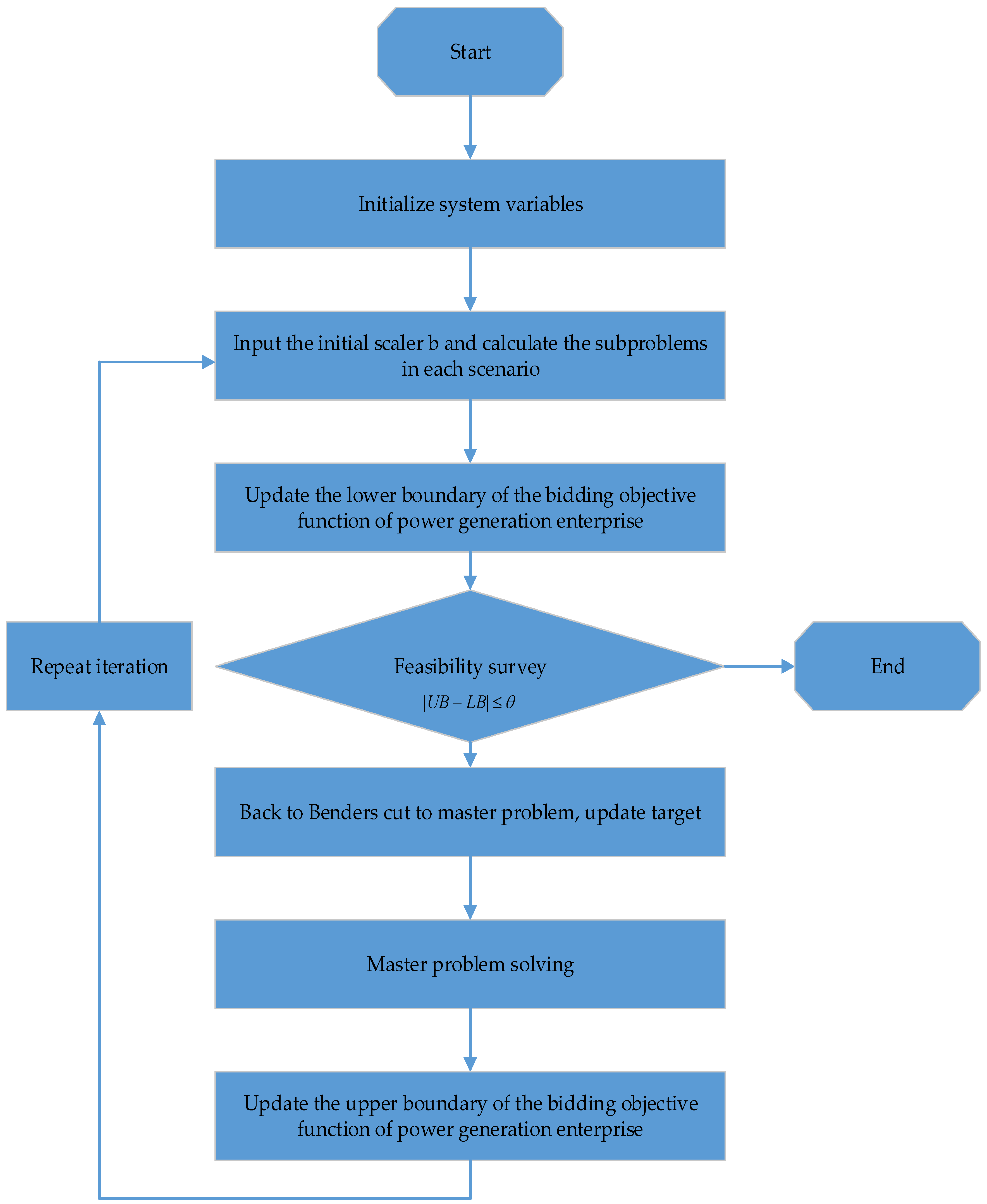
Because the two-stage stochastic optimization model of power generation enterprise bidding established in this paper contains the constraints of unit startup and shutdown, it cannot be solved directly by the classical Benders decomposition algorithm. Therefore, a convex hull approximation method is proposed for the feasible domain of sub-problems, which realizes the convexity of the feasible region of the sub-problem, as shown in Figure 4.

According to Figure 4, the improved Benders decomposition method can be used to calculate the two-stage optimization model of power generation enterprise bidding. The specific process is as follows.

Step 1:

Initialize the upper bound $LB=+\infty$ and the lower bound $UB=0$, and set the maximum tolerance of the difference between the upper and lower bounds $\theta$.

Step 2:

Enter a set of initial bid amount $b$ and calculate Sub-Questions (17) in each scenario, obtain the optimal value $b$, and update the lower bound $UB$ of the original problem.

Step 3:

Substitute the optimal value $Y^s$ in the second step into Equation (18) for solving, and construct Constraint (19).

Step 4:

Substitute Constraint (19) into model (18) and relax the constraint which restricts the type of variable $Y^s$. Then we can obtain model (20), which is a linear program. Solve model (20) and construct the benders cut based on the optimal values of its dual variables. The benders cut is then substituted into the master problem (16) so that the master problem is updated. Solve the new master problem and update the upper bound $LB$.

Step 5:

Observe if $UB-LB\le \theta$ is satisfied. If it is satisfied, the quality of the solution satisfies the decision-maker’s requirement, that is, the difference between the obtained optimal objective function value and the true optimal objective function value does not exceed $\theta$. The calculation is stopped, and the current result is output as the optimal solution. Otherwise, substitute the obtained one into the sub-problem and return to Step 2.

6. Case Analysis

6.1. Basic Date

This section introduces the data needed for the analysis of the example. This paper draws on a data from the Latin American (including Savardo, Honduras, and Nicaragua) wholesale electricity markets provided by [8]. Since there are too many parameters related to the clearing price of the electricity market, it cannot be enumerated in detail and can be obtained by referring to [8]. The parameters of the two thermal power units held by the price maker are derived from [27], as shown in

Table 1. The parameters of thermal power units.

Nominal Capacity (MW)	Number of Thermal Power Units (units)	Minimum Output (MW)	Climbing Speed (MW/h)	Downhill Speed (MW/h)
1200	10	400	600	600
1000	10	300	500	500
A (Dollar/MW2h)	B (Dollar/MWh)	C (Dollar/h)	Start-up cost (Dollar/per)	Shut-down cost (Dollar/per)
0.00148	1.2136	82	1600	1000
0.00289	1.2643	49	1400	800

. Quadratic function Ax² + Bx + C is used to formulate the generation cost of thermal power units. Thus, A, B, and C in Table 1 correspond to the coefficient of generation cost function of each thermal power unit.

Assume that the two units are turned off at the beginning of the scheduling period and are allowed to start immediately. The method for generating the wind power scene is as follows:

(1)

Use the nuclear density estimation method to analyze the historical data of wind power and obtain its approximate probability distribution function.

(2)

Use the Latin hypercube sampling method to discretize the probability distribution function and generate a wind power scene tree.

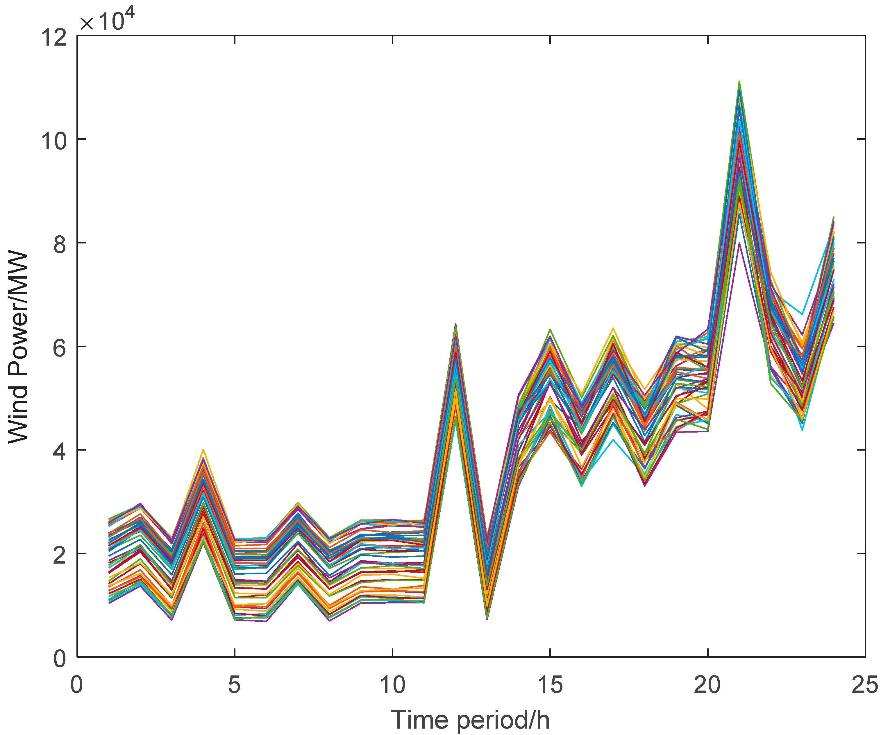
(3)

In order to avoid too many scenes, the back-generation reduction method is used to pre-process the scene, merge similar scenes, and finally obtain 50 wind power scenes, as shown in Figure 5 below.

The YALMIP toolbox [28] is a free toolbox based on the Matlab R2017a platform proposed by Dr. Johan Lofberg. It has a wide range of applications. In solving the optimization problem, it shows obvious advantages. One is that you can not only use the internal solution algorithm but also call other commercial solvers, such as CPLEX, GLPK, and Gurobi, which may greatly improve the ability to solve optimization problems. The YALMIP toolbox separates the modeling from the algorithm by simply setting parameters and specifying a solver. Based on this, the model uses the YALMIP toolbox to call the Gurobi 8.0 solver via the Matlab R2017a platform, which is equipped with an Intel(R) Core(TM) [email protected] GHZ CPU, 16 GB. In addition, the maximum error tolerance of the Benders decomposition algorithm is set to 0.001.

6.2. Results and Discussion

6.2.1. Additional Power Purchase Cost vs. Wind Curtailment Cost

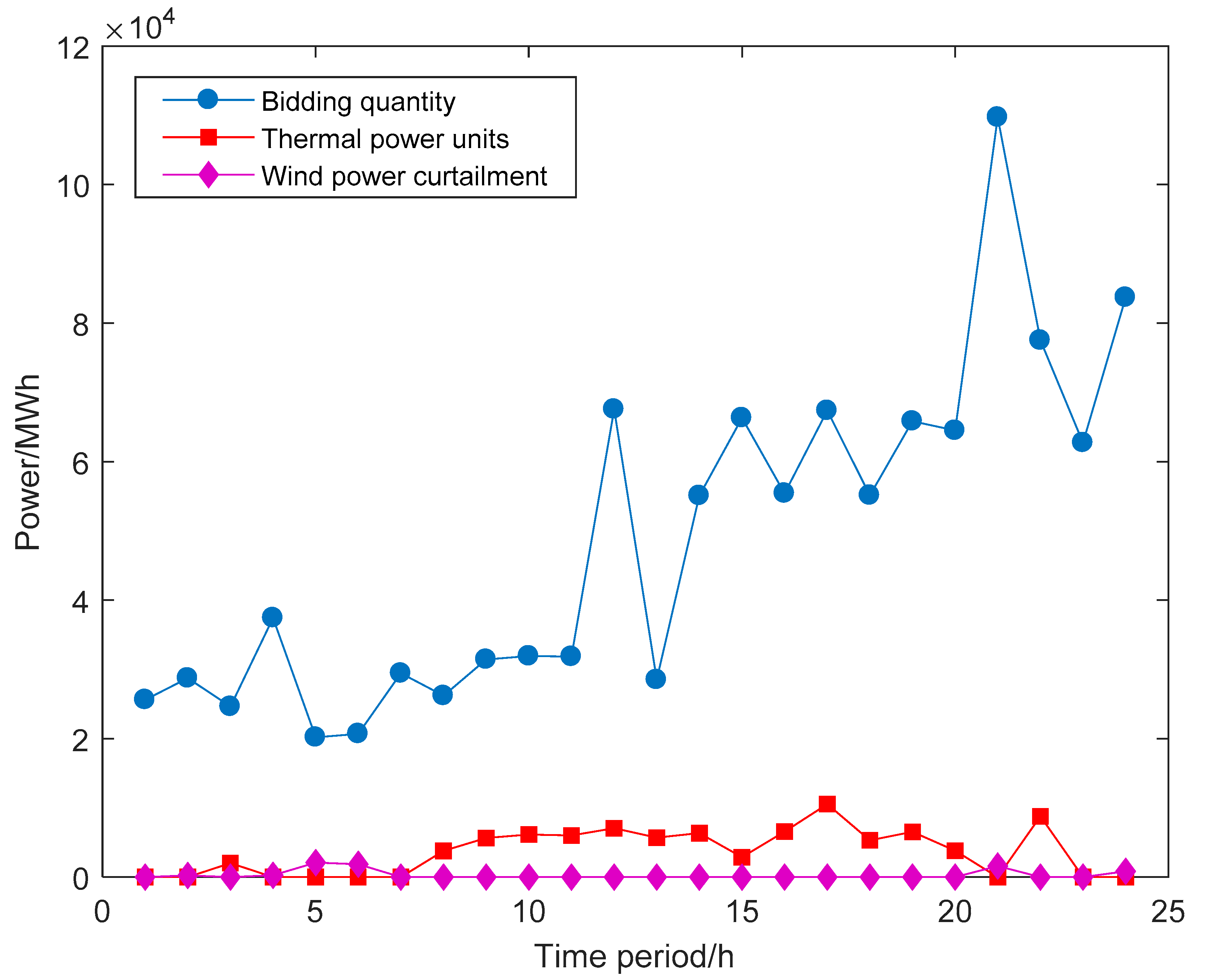
Since generation companies do not know the exact value of wind power in each time period, one of the most important problems in strategic bidding is the trade-off between the additional power purchase cost and the wind curtailment cost. If the bidding quantity is too high, generation companies are unable to satisfy the electricity demand by themselves in scenarios where the wind power output is low. They must purchase the electricity from other places, leading to the additional cost. However, if the bidding quantity is too low, the output of generation companies may also exceed the bidding quantity, so that extra wind power will be abandoned, leading to the wind curtailment cost. We are interested in the following question: Should generation companies select an aggressive decision with a high bidding quantity or a conservative decision with a low bidding quantity? We selected two scenarios from the set of these 50 scenarios, and the differences in scheduling decisions of power generation companies between these two scenarios were observed. As shown in Figure 6 and Figure 7, one scenario is the most optimistic, which means the wind power output during the entire horizon is the highest among all scenarios. Another scenario is the most pessimistic scenario, which means the wind power output during the entire horizon is the lowest among all the scenarios.

Figure 6 shows the optimal results in the most optimistic scenario. The additional power purchase is 0 during the entire planning horizon. Wind power curtailment quantities are also 0 in most time periods. Even if in some periods the wind curtailment quantities are not 0, they are relatively low compared with the bidding quantities in these time periods. As for the thermal power units, their generation quantities do not reach their maximum limitation in most time periods.

Figure 7 shows the optimal results in the most pessimistic scenario. Different from the most optimistic scenario, the wind curtailment quantities are 0 during the entire planning horizon. Although the generation quantities of all thermal power units reach their maximum limitation, generation companies still need to purchase additional power in all time periods. The generation quantities of thermal power units do not reach their maximum limitation during Time Periods 5 and 6. This is because the market-clearing price in Time Periods 5 and 6 is lower than the unit generation cost of these thermal power units. One can refer to Figure 8 to see the market-clearing prices during the entire planning horizon.

(1)

Thermal power units play a significant role in coping with wind power uncertainty. In the most optimistic scenario where the wind power is high, the generation company reduces the generation quantities of thermal power units. Since the unit generation cost of wind power is much cheaper than the thermal power, most electricity demands are satisfied through wind power in order to save the generation cost. On the contrary, in the most pessimistic case, where the wind power is low, the generation company increases the generation quantities of thermal power units in the case of an additional power purchase cost.

(2)

Aggressive bidding quantities, compared with conservative bidding quantities, are preferred by the generation company. Note that, even in the most optimistic case, the wind power curtailment is still very low. However, in the most pessimistic case, the additional power purchase is relatively high. If a generation company offers low bidding quantities in the day-ahead electricity market, it will not only suffer the wind curtailment cost in some scenarios when wind power is high but also lose the opportunity of earning more revenue. Therefore, a generation company would rather offer high bidding quantities since the loss of revenue and wind curtailment cost is much higher than the additional power purchase cost.

Figure 6 and Figure 7 lead to the following conclusions.

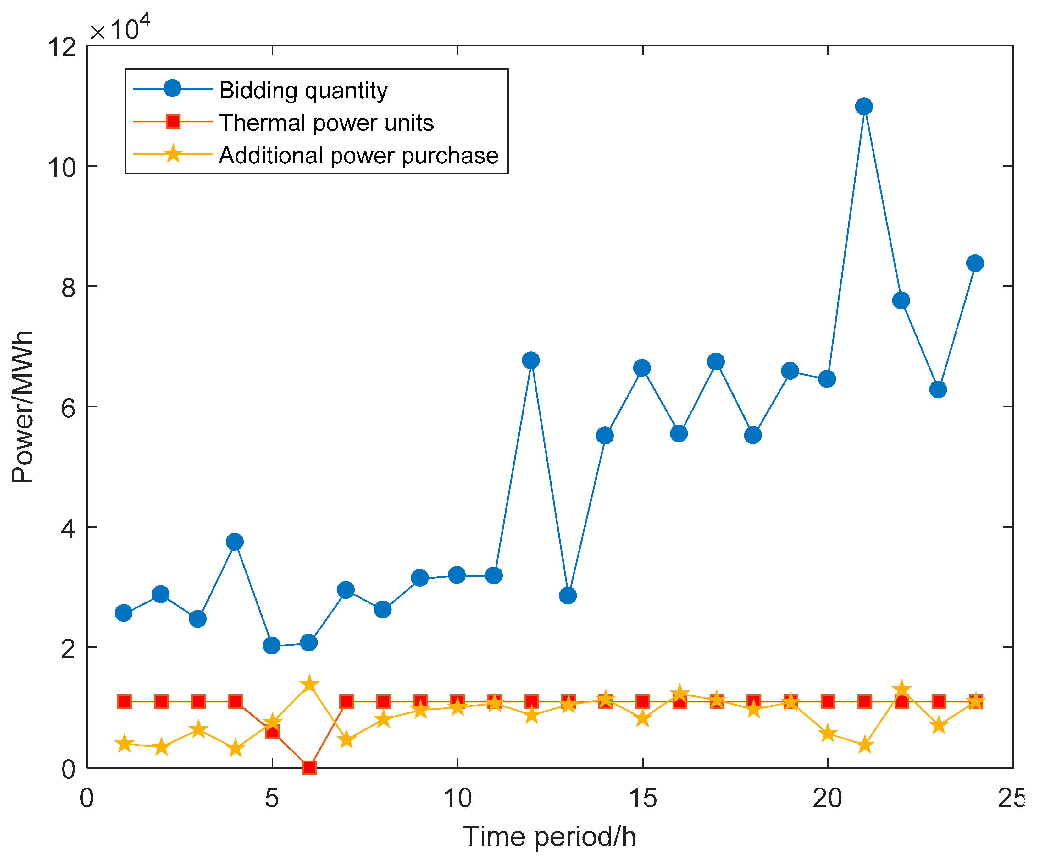
6.2.2. The Effect of Additional Power Purchase on Decision-Makings

In the strategic bidding of generation companies, many models have an important assumption that the generation quantities of a power generation company in some time period do not have to equate to its bidding quantity. If a generation company cannot produce that much electricity, it is allowed to purchase the electricity from other places, with a higher unit price compared with the market-clearing price. However, additional power purchases are not always possible, especially when the power generation company is a price maker with the largest installed capacity. In this case, other price takers may not able to provide enough electricity to fill the gap between bidding quantity and generation quantity for price makers. Based on the above consideration, we discuss the effect of additional power purchases on decision-makings. The effect of additional electricity on decision-makings is shown in

Table 2. The effect of additional electricity on decision-makings.

Y/N	Expected Profit (Dollar)	Total Bidding Quantity (MWh)	Expected Additional Power Purchase (MWh)	Wind Power Curtailment (MWh)
Y	4.38 × 108	1.17 × 106	5.82 × 104	269.99
N	4.00 × 108	9.54 × 105	0	2.97 × 104

.

Table 2 shows that, if an additional power purchase is allowed, the expected profit of the generation company is much higher. This generation company also offers higher bidding quantities in the day-ahead electricity market. The expected wind curtailment will be much higher if an additional power purchase is not allowed.

The comparison shows that an additional power purchase provides a generation company with high flexibility in its decision-making. Note that an important feature of two-stage stochastic optimization theory is the robustness of the constraints, i.e., the constraints must be satisfied in all scenarios. As mentioned earlier, we find that a generation company always prefers high bidding quantities when an additional power purchase is allowed. This is because, even if the generation quantities of the generation company cannot satisfy the bidding quantity, a generation company is allowed to purchase electricity from other places to fill the gap. However, if an additional power purchase is not allowed, the generation company must offer lower bidding quantities in case of a violation of power balance constraints. Note that wind power in some scenarios may exceed these low bidding quantities, which lead to a higher expected wind power curtailment.

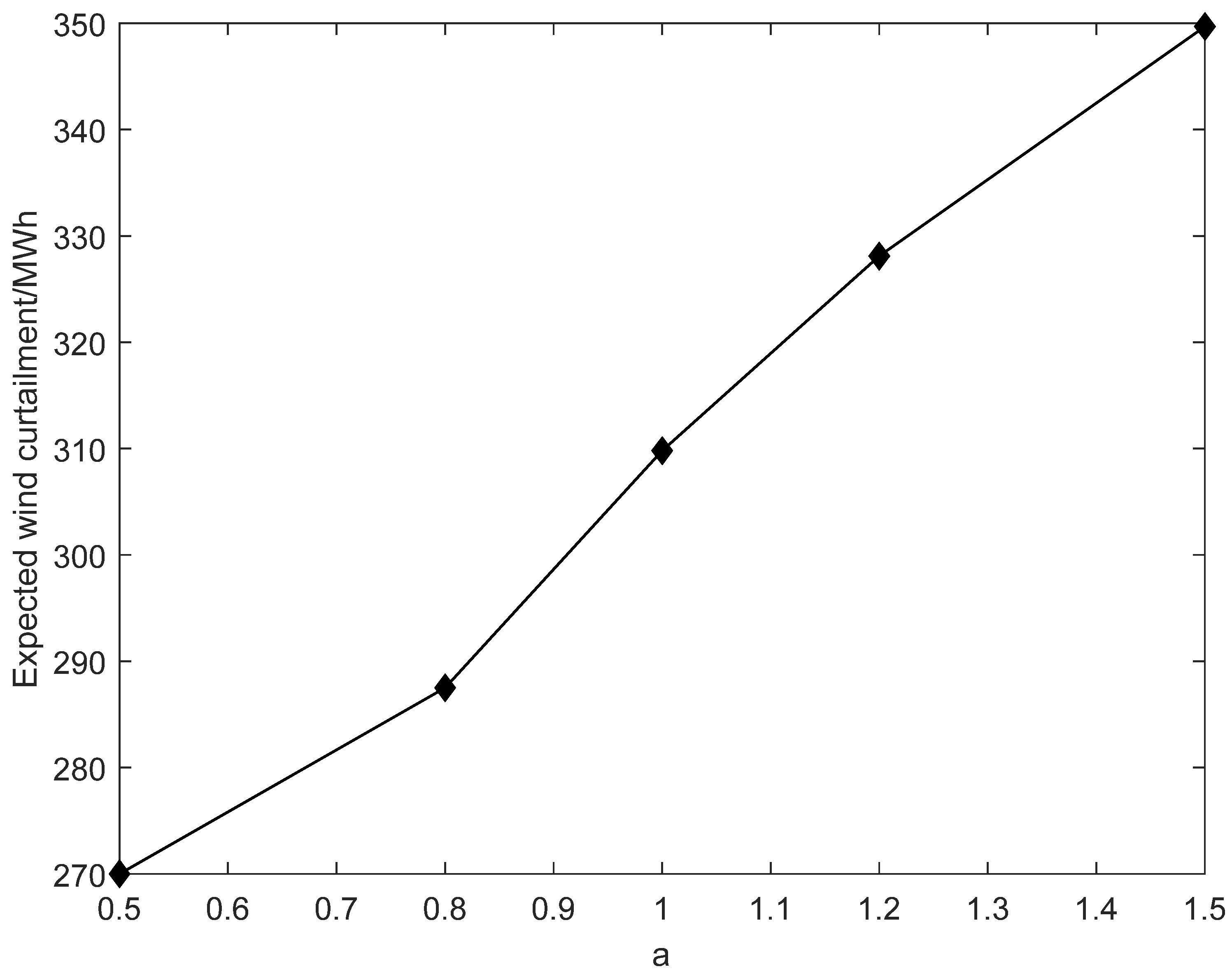
6.2.3. The Effect of Wind Power Volatility on Decision-Makings

One of the important purposes of the two-stage stochastic optimization model is to help power generation companies deal with wind power uncertainty. Note that wind power uncertainty can be characterized by its variance, which is used to measure the expectation of the squared deviation of a random variable from its mean. Based on this consideration, sensitivity analyses with regard to the variance of wind power is conducted. Assume that the variance of wind power in the original case is ${\sigma }^2$. We use $a{\sigma }^2$ to represent the variance of wind power in different cases. By changing the value of a, the sensitivity analyses of the variance of wind power are realized. The results are shown in

Table 3. The effect of the variance of wind power on decision-makings.

a	Expected Profit (Dollar)	Total Bidding Quantity (MWh)	Expected Additional Power Purchase (MWh)	Expected Discarding Electricity (MWh)
0.5	4.38 × 108	1.17 × 106	5.82 × 104	269.99
0.8	4.27 × 108	1.14 × 106	5.87 × 104	287.45
1.0	4.15 × 108	1.10 × 106	5.93 × 104	309.78
1.2	4.00 × 108	1.06 × 106	5.98 × 104	328.14
1.5	3.80 × 108	1.00 × 106	6.04 × 104	349.61

and Figure 9.

Table 3 and Figure 9 shows that, even if the expectations of wind power are maintained and only the variance is increased, the decision-making of power generation companies will become more and more conservative and the profit is expected to be lower and lower. This is related to the robustness of the electric balance expressed by Constraint (3). When the variance of the wind power increased, the amount of wind power generated under the “worst case” is reduced. Since Constraint (3) guarantees that the bidding amount of the power generation company must be satisfied even in the “worst scenario,” the power generation enterprise has to reduce the bid amount to meet the “worst case scenario” requirement. The computational results show that reducing the forecasting error of wind power is significant for the strategic bidding of generation company.

In order to show the rationality and effectiveness of the proposed algorithm in dealing with the model, two kinds of methods are used to solve the model, and the efficiency of the solution under different methods is compared. In the first case, the improved Benders decomposition algorithm is used, and in the second the Gurobi 8.0 solver is directly called to solve the model. In order to improve the solution dimension of the sub-problem, the number of thermal power units held by power generation enterprises is increased to 20, and the proportion of wind power generation is adjusted accordingly. The maximum allowable CPU time is 3600 s. If the result is still not obtained after 3600 s, the solution is considered unsuccessful. The result is shown in Figure 10.

Figure 10 shows that, when the number of scenarios is small, the advantages of the improved Benders decomposition algorithm are not obvious, and in some cases the efficiency is even lower than the direct solution (branch and bound). However, as the number of scenario increases, the advantages of improving the Benders decomposition algorithm begin to manifest. When the number of scenario exceeds 150, it is impossible to obtain the optimal solution by direct solution in the CPU time of 1800 s. However, even if the number of scenario reaches 300, the Benders decomposition still shows a correspondingly better solution efficiency. It can be seen that the improved Benders decomposition algorithm is reasonable and effective for the model constructed in this paper.

7. Conclusions

This paper examines the bidding of power generation companies with wind and thermal power units in a free deregulated electricity market. Considering that the decisions of the power generation companies can be divided into day-ahead market bidding decisions and unit combination decisions, this paper constructs a two-stage stochastic optimization model considering wind power uncertainty and unit combination constraints. From the solution results, the following conclusions can be drawn:

(1)

The key to strategic bidding is the tradeoff between high bidding quantities and low bidding quantities. Too much or too little bidding can result in loss for a generation company. Various factors discussed in the examples will have an impact on the bidding quantities of power generation companies. In addition, unless the cost of additional electricity purchases is high enough, power generation companies will be more inclined to make aggressive decisions to avoid the loss of opportunity costs due to excessive power abandonment.

(2)

The goal of power generation companies is to maximize their expected benefits. However, even if we do not change the expected value of wind power but only increase their volatility, it will still cause the expected profit of power producers to decrease.

(3)

Properly retaining a certain proportion of thermal power units is important for promoting wind power consumption and improving the profitability of power generation companies.

References

1. Xu, T. 2017 Global Wind Power Installed Capacity Statistics. Wind. Energy Ind. 2018, 3, 51–57. [Google Scholar]
2. Yucekayaa, A.D.; Valenzuelaa, J.; Dozierb, G. Strategic bidding in electricity markets using particle swarm optimization. Electr. Power Syst. Res. 2009, 79, 335–345. [Google Scholar] [CrossRef]
3. Bompard, E.; Ma, Y.; Napoli, R.; Abrate, G. The Demand Elasticity Impacts on the Strategic Bidding Behavior of the Electricity Producers. IEEE Trans. Power Syst. 2007, 22, 188–197. [Google Scholar] [CrossRef]
4. Barroso, L.A.; Carneiro, R.D.; Granville, S.; Pereira, M.V.; Famp, M.H.C. Nash Equilibrium in Strategic Bidding: A Binary Expansion Approach. IEEE Trans. Power Syst. 2006, 21, 629–638. [Google Scholar] [CrossRef] [Green Version]
5. Li, T.; Shahidehpour, M. Strategic Bidding of Transmission-Constrained GENCOs with Incomplete Information. IEEE Trans. Power Syst. 2005, 20, 437–447. [Google Scholar] [CrossRef]
6. Lamont, J.W.; Rajan, S. Strategic bidding in an energy brokeragy. IEEE Trans. Power Syst. 1997, 12, 1729–1733. [Google Scholar] [CrossRef]
7. Pereira, M.V.; Granville, S.; Fampa, M.H.C.; Dix, R.; Barroso, L.A. Strategic Bidding under Uncertainty: A Binary Expansion Approach. IEEE Trans. Power Syst. 2005, 20, 180–188. [Google Scholar] [CrossRef]
8. Kazemi, M.; Mohammadi-Ivatloo, B.; Ehsan, M. Risk-based bidding of large electric utilities using Information Gap Decision Theory considering demand response. Electr. Power Syst. Res. 2014, 114, 86–92. [Google Scholar] [CrossRef]
9. Ren, Y.L.; Zou, X.Y.; Zhang, X.H. Bidding game model of power generation company based on first-price sealed auction. J. Syst. Eng. 2003, 18, 248–254. [Google Scholar]
10. Bushnell, J. A mixed complementarity model of hydrothermal electricity competition in the western United States. Oper. Res. 2003, 51, 80–93. [Google Scholar] [CrossRef]
11. Ding, H.J.; Pinson, P.; Hu, Z.C. Integrated bidding and operating strategies for wind-storage systems. IEEE Trans. Sustain. Energy 2016, 7, 163–172. [Google Scholar] [CrossRef]
12. De la Nieta, A.A.S.; Contreras, J.; Muñoz, J.I. Optimal coordinated wind-hydro bidding strategies in day-ahead markets. IEEE Trans. Power Syst. 2013, 28, 798–809. [Google Scholar] [CrossRef]
13. Yan, J.; Liu, Y.Q.; Han, S.; Wang, Y.M.; Feng, S.L. Reviews on Uncertainty Analysis of wind Power Forecasting. Renew. Sustain. Energy Rev. 2015, 52, 1322–1330. [Google Scholar] [CrossRef]
14. Li, H.; Zhang, R.C.; Wang, X.S.; Dong, Y. Multi-Time Scale Rolling Economic Dispatch for Wind/Storage Power System based on forecast Error Feature Extraction. Energies 2018, 11, 2124. [Google Scholar]
15. Zhang, X.H.; Yan, K.L.; Lu, Z.G.; Zhong, J.Q. Scenario Probability Basted Multi-Objective Optimized Low-Carton Economic Dispatching for Power Grid Integrated with Wind Farms. Power Syst. Technol. 2014, 38, 1835–1841. [Google Scholar]
16. Bin, J.; Yuan, X.H.; Chen, Z.H.; Tian, H. Improved gravitational search algorithm for unit commitment considering uncertainty of wind power. Energy 2014, 67, 52–62. [Google Scholar]
17. Jiang, R.; Wang, J.H.; Guan, Y.P. Robust unit commitment with wind power and pumped storage hydro. IEEE Trans. Power Syst. 2012, 27, 800–810. [Google Scholar] [CrossRef]
18. Fu, Y.; Chen, T.; Li, Z.K.; Wei, S.R.; Ji, L. Robust Security Economic Dispatch Considering Wind Power Curtailment. Proc. CSEE 2017, 37, 47–54. [Google Scholar]
19. Lorca, Á.; Sun, X.A. Adaptive Robust Optimization With Dynamic Uncertainty Sets for Multi-Period Economic Dispatch Under Significant Wind. IEEE Trans. Power Syst. 2015, 30, 1702–1713. [Google Scholar] [CrossRef]
20. Sun, Y. Ultra-Short Term Dispatching Strategies for the System with Large-Scale Wind Power Integration; Northeast Electric Power University: Jilin, China, 2018. [Google Scholar]
21. Tan, Z.F.; Li, H.H.; Ju, L.W.; Song, Y.H. An Optimization Model for Large-Scale Wind Power Grid Connection Considering Demand Response and Energy Storage Systems. Energies 2014, 7, 7282–7304. [Google Scholar] [CrossRef]
22. Zhao, C.Y.; Wang, Q.F.; Wang, J.H. Expected Value and Chance Constrained Stochastic Unit Commitment Ensuring Wind Power Utilization. IEEE Trans. Power Syst. 2014, 29, 2696–2705. [Google Scholar] [CrossRef]
23. Liu, B.; Liu, F.; Wang, C.; Mei, S.; Wei, W. Uncertainty Set Modeling and Evaluation of Wind Farm Power Output for Robust Dispatch. Autom. Electr. Power Syst. 2015, 39, 8–14. [Google Scholar]
24. Guan, Y.P.; Wang, J.H. Uncertainty Sets for Robust Unit Commitment. IEEE Power Energy Soc. 2014, 29, 1439–1440. [Google Scholar] [CrossRef]
25. Hu, B.Q.; Wu, L.; Marwali, M. On the Robust Solution to SCUC with Load and Wind Uncertainty Correlations. IEEE Trans. Power Syst. 2014, 29, 2952–2964. [Google Scholar] [CrossRef]
26. Damodaran, S.K.; Kumar, T.K.S. Hydro-Thermal-Wind Generation Scheduling Considering Economic and Environmental Factors Using Heuristic Algorithms. Energies 2018, 11, 353. [Google Scholar] [CrossRef]
27. Carrion, M.; Arroyo, J.M. A computationally efficient mixed-integer linear formulation for the thermal unit commitment problem. IEEE Trans. Power Syst. 2006, 21, 1371–1378. [Google Scholar] [CrossRef]
28. Löfberg, J. YALMIP: A toolbox for modeling and optimization in MATLAB. In Proceedings of the 2004 IEEE International Symposium on Computer Aided Control Systems Design, New Orleans, LA, USA, 2–4 September 2004; pp. 284–289. [Google Scholar]
Figure 1. Demand and supply in the electricity wholesale market.
Energies 11 03527 g001
Figure 2. The function diagram of the return of the price taker.
Energies 11 03527 g002
Figure 3. The process of two-stage decision-making.
Energies 11 03527 g003
Figure 4. The flow chart to solve the two-stage stochastic optimization model of power generation enterprise bidding based on the improved Benders decomposition method.
Energies 11 03527 g004
Figure 5. The scenarios of wind power.
Energies 11 03527 g005
Figure 6. The optimal decision-making under the most optimistic scenario.
Energies 11 03527 g006
Figure 7. The optimal decision-making under the most pessimistic scenario.
Energies 11 03527 g007
Figure 8. The market-clearing price during the entire planning horizon.
Energies 11 03527 g008
Figure 9. The expected wind power curtailment with different values of parameter a.
Energies 11 03527 g009
Figure 10. Computation efficiency.
Energies 11 03527 g010