Analyzing the Near-Field Effects and the Power Production of an Array of Heaving Cylindrical WECs and OSWECs Using a Coupled Hydrodynamic-PTO Model

Abstract

The Power Take-Off (PTO) system is the key component of a Wave Energy Converter (WEC) that distinguishes it from a simple floating body because the uptake of the energy by the PTO system modifies the wave field surrounding the WEC. Consequently, the choice of a proper PTO model of a WEC is a key factor in the accuracy of a numerical model that serves to validate the economic impact of a wave energy project. Simultaneously, the given numerical model needs to simulate many WEC units operating in close proximity in a WEC farm, as such conglomerations are seen by the wave energy industry as the path to economic viability. A balance must therefore be struck between an accurate PTO model and the numerical cost of running it for various WEC farm configurations to test the viability of any given WEC farm project. Because hydrodynamic interaction between the WECs in a farm modifies the incoming wave field, both the power output of a WEC farm and the surface elevations in the ‘near field’ area will be affected. For certain types of WECs, namely heaving cylindrical WECs, the PTO system strongly modifies the motion of the WECs. Consequently, the choice of a PTO system affects both the power production and the surface elevations in the ‘near field’ of a WEC farm. In this paper, we investigate the effect of a PTO system for a small wave farm that we term ‘WEC array’ of 5 WECs of two types: a heaving cylindrical WEC and an Oscillating Surge Wave Energy Converter (OSWEC). These WECs are positioned in a staggered array configuration designed to extract the maximum power from the incident waves. The PTO system is modelled in WEC-Sim, a purpose-built WEC dynamics simulator. The PTO system is coupled to the open-source wave structure interaction solver NEMOH to calculate the average wave field $\eta$ in the ‘near-field’. Using a WEC-specific novel PTO system model, the effect of a hydraulic PTO system on the WEC array power production and the near-field is compared to that of a linear PTO system. Results are given for a series of regular wave conditions for a single WEC and subsequently extended to a 5-WEC array. We demonstrate the quantitative and qualitative differences in the power and the ‘near-field’ effects between a 5-heaving cylindrical WEC array and a 5-OSWEC array. Furthermore, we show that modeling a hydraulic PTO system as a linear PTO system in the case of a heaving cylindrical WEC leads to considerable inaccuracies in the calculation of average absorbed power, but not in the near-field surface elevations. Yet, in the case of an OSWEC, a hydraulic PTO system cannot be reduced to a linear PTO coefficient without introducing substantial inaccuracies into both the array power output and the near-field effects. We discuss the implications of our results compared to previous research on WEC arrays which used simplified linear coefficients as a proxy for PTO systems.

1. Introduction

Ocean Wave Energy is a potential source of clean electricity that can make a significant contribution to the de-carbonization of the world’s electricity supply. However, for it to follow the path of offshore wind and become a commercially viable power source, significant cost reductions need to be made. Because of practical limitations on the physical size of an individual Wave Energy Converter (WEC), these devices must be placed in close proximity to benefit from economies of scale such as those witnessed in the offshore wind industry. Such agglomerations of WECs are commonly termed wave farms. To match the power output of offshore wind farms, WEC farms need to consist of hundreds of WECs. How these WECs are grouped and arranged within a wave farm to maximize profitability while minimizing detrimental effects is still an open question.

Due to hydrodynamic interactions between individual WECs and closely spaced groups of WECs, determining the power output of a WEC farm is not a trivial matter. Unlike the case of wind farms, the interactions can be both beneficial and deleterious and correctly modelling them can make or break the financial viability of a WEC farm. As experimental studies are costly and time consuming, the chief design tool for assessing WEC farms is numerical modelling. There are many variables influencing the estimated power output, among them the site wave climate and bathymetry, WEC farm layout and the Power Take-off (PTO system) of each WEC. Modelling them in parallel leads to significant demands on computational power, and often leads to unclear conclusions. An additional complication for the numerical modelers is that many of the aforementioned variables are interdependent; it is, therefore, essential to understand the significance of each of the variables underlying the chosen numerical model.

For a given WEC type and for a given incident wave, a critical parameter that influences the WEC motion and the power output of a WEC farm is the PTO system. Because of the variety of technical solutions and the complexity of modeling the inherently non-linear behavior of most viable PTO systems in WECs, a plurality of previous investigations has assumed a simple mechanical damper as a proxy for the PTO system. Some examples for farms of heaving cylindrical WECs are found in [1,2,3,4,5] and for Oscillating Surging Wave Energy Converters (OSWECs) in [6,7,8,9]. Concurrently, due to step improvements in hydrodynamic modelling software, there has been a jump in the number of numerical investigations that have modelled single WECs [10,11,12,13] and small farms of WECs [14,15] with fully non-linear hydrodynamics. Yet, as pointed out in Penalba et al. [16] for the case of heaving point absorbers and in [8] for OSWECs, the errors due to a simplified PTO model can override any improvements made by more accurate hydrodynamic models. A particular concern with many existing PTO modelling efforts is that the most common PTO system type developed for commercial WEC prototypes, a hydraulic PTO system, is inherently non-linear [17,18]. A few recent studies, notably [16,17,18,19,20,21,22] have implemented realistic hydraulic PTO models with non-linear dynamics. However, these studies were limited in their scope to single WECs and not WEC farms, furthermore, many of the models quite complicated in their implementation.

In this paper, our aim is to implement a realistic hydraulic PTO model for two types of promising WEC technologies, namely heaving cylindrical WECs and OSWECs, in an array composed of 5 WECs. Although the terms WEC farm and WEC array are used interchangeably, we will follow the precedent set in [23] and term a small farm of closely spaced WECs a WEC array. The impact of the hydraulic PTO system on the power output and the ‘near-field’ surface elevations of the 5-WEC array is compared to that of the base case of a linear PTO system. Both PTO systems are simulated using WEC-Sim [6], a dynamical simulator for WECs built in the MATLAB Simulink platform. The PTO model is coupled to the open-source wave-structure interaction solver NEMOH [24] using the perturbed wave field imparted by the motion of the WECs in WEC-Sim. Previously, a similar approach was presented in [25,26,27] for the case of a wave-structure interaction solver coupled to a wave propagation model using a basic linear PTO model. WEC-Sim has been used in modelling hydraulic PTOs in several recent studies [20,22]. In the present paper, only the near-field zone is simulated with a future goal of coupling to a wave propagation model to model the impact of a WEC farm (consisting of one or multiple WEC arrays) in the ‘far-field’. In referencing the near-field we refer to the area inside the WEC array immediately surrounding the WECs, while the far-field can refer to areas outside the immediate area of the WEC array up to several km away. The modifications of the wave field in the presence of multiple bodies are referred to as ‘array effects’, that are synonymous with ‘farm’ or ‘park effects’ used in some literature [2,28,29,30]. We begin by listing the underlying theory and assumptions in Section 2. Then we provide the details on the two numerical PTO system interpretations used in the study in Section 3 and specify the regular wave test matrix of the simulations in Section 4.2. We then present the results for a single WEC for the power in Section 5.1, the near-field $|\eta |$ in Section 5.2 and compare the performance and effects of a hydraulic PTO system to a linear PTO system in Section 5.2.3. Next, we present the corresponding results for the 5-WEC arrays of heaving cylindrical WECs and OSWECs in Section 6.4, Section 6.5 and Section 6.5.3. Finally, we highlight the key messages of the research in the discussion in Section 7 and make conclusions with a view toward a continuation of the work undertaken in this paper in Section 8.

2. Hydrodynamic Model Description

2.1. Linear Potential Flow

This investigation assumes linear potential flow theory [31], a subset of linear wave theory that allows the fluid velocity, v, to be expressed as the gradient of the time dependent potential $\mathsf{\Phi }$, (Equation (1)).

$$v=\nabla \mathsf{\Phi }$$

(1)

The assumptions underlying potential flow are the following:

• the fluid is inviscid;
• the fluid is incompressible; and
• the flow is irrotational.

The standard assumption of linear theory that the motion amplitudes of the bodies are much smaller than the wavelength also applies. Linear potential flow theory has hitherto been used in most of the investigations into WEC array modelling, for example see [3,29,30,32]. In further assuming that all time-varying quantities oscillate with the same angular frequency $\omega$, we can separate out the time dependence from the time-independent velocity potential $\varphi$,

$$\varphi (x,y,z,t)=\Re \left\{\varphi (x,y,z)e^{-i\omega t}\right\}$$

(2)

where $\varphi$ is the complex velocity potential. Due to application of the principle of superposition, linear potential theory allows for the separation of the total velocity potential into the following components (Equation (3)):

$${\varphi }_t(x,y,z)={\varphi }_i+{\varphi }_d+\sum _i^6{\varphi }_r$$

(3)

where ${\varphi }_t$ is the total velocity potential, ${\varphi }_i$ is the incident wave velocity potential, ${\varphi }_d$ the diffracted wave velocity potential and ${\sum }_i^6{\varphi }_r$ is the sum of the radiated wave velocity potentials for each Degree of Freedom (DoF) of the WEC. In our investigation we only model 1 DoF for each WEC, namely heave for the cylindrical WEC and pitch for the OSWEC. We also introduce the term perturbed wave to denote the wave resulting from sum of the diffracted and radiated velocity potentials.

2.2. Boundary Element Method Solver

In our coupling approach the ‘array’ effects, induced by the hydrodynamic interaction between the WECs, are resolved by simulating the WEC motions using the open-source potential flow Boundary Element Method (BEM) solver NEMOH [24]. Given Equation (1), NEMOH solves the Laplace equation, Equation (4), for the complex velocity potential, $\varphi$:

$$\nabla \varphi =0$$

(4)

given a set of boundary conditions on the wetted body surface, the free surface, sea bottom and far-field. The equations of motion are solved using the method of Green’s functions, as explained in [24]. An important restriction imposed by the method is the assumption that the water depth h is constant throughout the WEC array domain. The free surface elevation $\eta$ is calculated by taking the real part of the complex surface elevation $\overline{\eta }$ that is in turn obtained in NEMOH from the free surface boundary condition Equation (5). From the superposition principle of Equation (3), free surface elevations $\eta$ can be obtained separately for the WEC motions due to the diffracted and the radiated potentials:

$$\eta =-\frac{1}{g}{\left(\frac{\partial \varphi }{\partial t}\right)}_{z=0}$$

(5)

where g is the acceleration due to gravity and $z=0$ is the undisturbed free surface. NEMOH also calculates the coefficients of the added mass $A\left(\omega \right)$, hydrodynamic damping $B\left(\omega \right)$, and hydrodynamic restoring force or buoyancy force $K(\omega$) which are used to calculate the WEC motions in Section 3.1.

3. PTO Model Development

3.1. Equations of Motion

To model the WECs with a given PTO system, in this investigation we use the open source mechanical solver WEC-Sim developed by Sandia National Laboratory in collaboration with the National Renewable Energy Laboratory (NREL) in the US [6]. WEC-Sim operates within the MATLAB Simulink environment. For 1 DoF WEC displaced a distance z from equilibrium, WEC-Sim solves for the WEC motion in the time domain using the Cummins Equation (6):

$${\mathrm{M}}_t\ddot{z}\left(t\right)=f_e\left(t\right)+f_{rad}\left(t\right)+f_{hs}\left(t\right)+f_{PTO}\left(t\right)+f_v\left(t\right)+f_m\left(t\right)$$

(6)

In the case of a floating WEC oscillating in heave, ${\mathrm{M}}_t=\mathrm{M}+A_{33\infty }$ where M is the generalized mass matrix and $A_{33\infty }$ is the asymptotic value of the heave added mass. On the right hand side, $f_e\left(t\right)$ is the excitation force, $f_{PTO}\left(t\right)$ is the PTO force, $f_{hs}\left(t\right)$ is the hydrostatic force, $f_{rad}\left(t\right)$ is the force vector of radiation, $f_v\left(t\right)$ are the forces that can be modelled as viscous or friction losses in the system, and $f_m\left(t\right)$ is the force vectors resulting from the mooring connections. The excitation force is calculated as $f_e\left(t\right)={\mathcal{F}}^{-1}\left\{F_e\left(\omega \right)\eta (\omega )\right\}$, where $\eta \left(\omega \right)$ is the Fourier transform of the surface elevation and $F_e\left(\omega \right)$ is the frequency domain exciting force transfer function. $f_{hs}\left(t\right)$ is the hydrostatic force which is equal to $K_{33}Z\left(\omega \right)$ where $K_{33}$ represents the hydrostatic stiffness and $Z\left(\omega \right)$ the frequency domain displacement of the heaving cylindrical WEC. The hydrodynamic coefficients representing A, the added mass of the device, B, the hydrodynamic damping and K, the hydrodynamic spring or stiffness, are calculated in the frequency domain in NEMOH for each relevant degree of freedom for the given WECtype. Please note that henceforth all capital letters represent frequency domain complex quantities while small case letter real-valued time-domain quantities. For the regular waves simulated herein, the radiation force $f_{rad}\left(t\right)$ can be calculated in the steady state form for a given frequency $\omega$ by the following Equation (7):

$$f_{rad}\left(t\right)=-A\left(\omega \right)\ddot{z}-B\left(\omega \right)\dot{z}.$$

(7)

In this paper, we do not model $f_v\left(t\right)$ and $f_m\left(t\right)$ since they are assumed to be negligible, therefore those terms are set equal to zero. The OSWEC described in Section 4.1 is simulated using the same Equation (6), with the substitution of torques for the forces and the pitch angular displacement $\theta \left(t\right)$ for the heave displacement $z\left(t\right)$ and the coefficients in heave for the coefficients in pitch. Two different types of power take-off systems will be further discussed: a linear and hydraulic PTO system, the former being the most popular way of simplifying a PTO system while the latter being one of the most used PTO systems in commercial WEC designs.

3.1.1. Linear PTO System

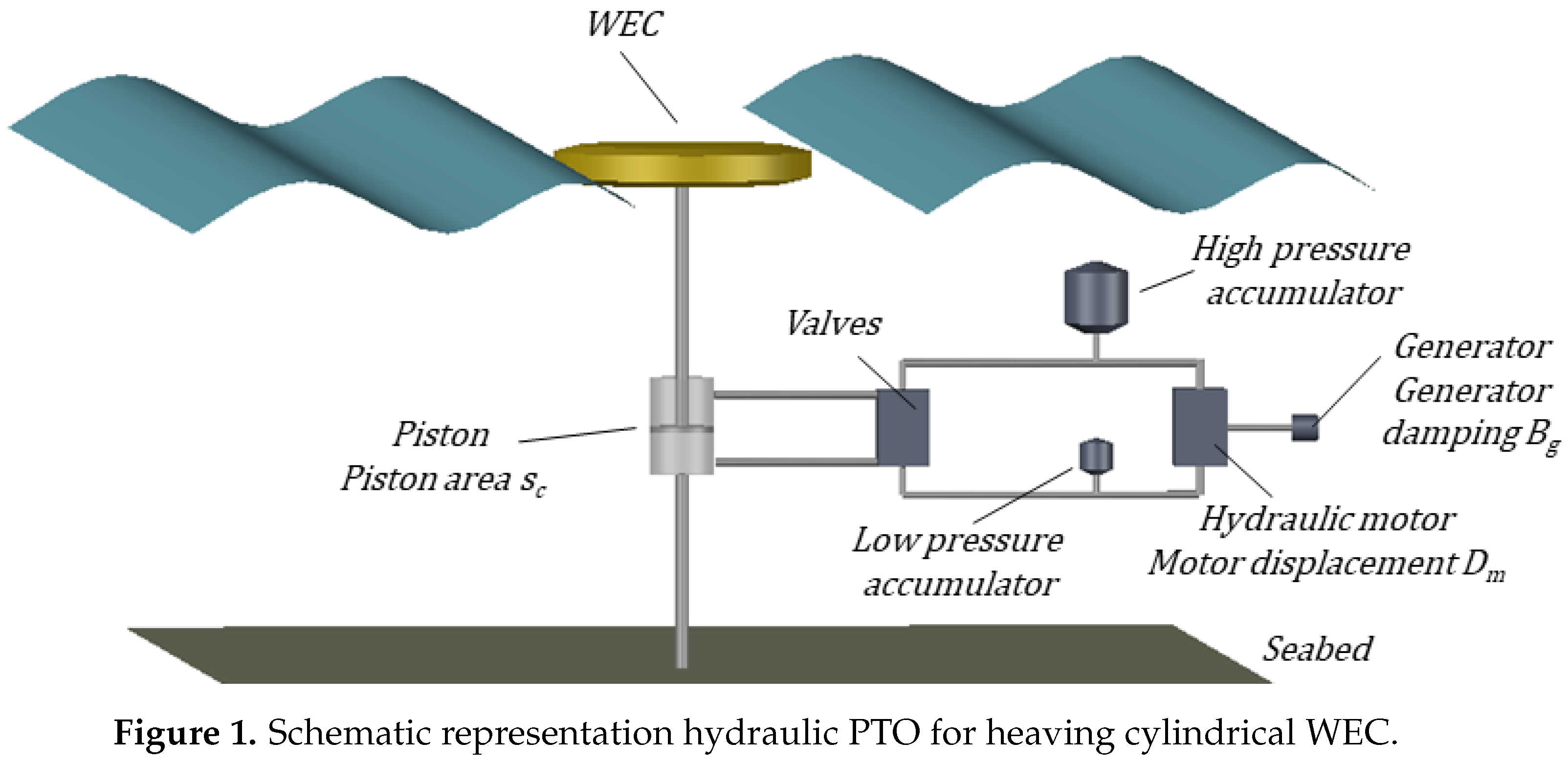
The most common way of simulating the effect of the PTO system of a wave energy converter is by modelling its dynamics as linear. This means the PTO system is modelled as a spring-damper-mass system with stiffness coefficient $K_{PTO}$ and damping coefficient $B_{PTO}$. However, because of the practical difficulty of changing the mass of the PTO system in real-time, it is often assumed the mass is unchangeable, resulting in the spring-damper system as represented in Figure 1 for the heaving cylindrical WEC. For practical reasons, a variable spring system is often difficult to implement, therefore a further simplification is warranted where we set the stiffness coefficient $K_{PTO}$ to zero. In the following calculations, the PTO system will be modelled as linear damper, resulting in the following expression for the PTO force:

$$f_{PTO,l}\left(t\right)=-B_{PTO,l}\dot{z}\left(t\right)$$

(8)

with $B_{PTO,l}$ the linear PTO damping term. The linear PTO influences the dynamics of the heaving cylindrical WEC: it exerts a force, $f_{PTO,l}\left(t\right)$, oppositely directed to the WEC’s velocity, $\dot{z}\left(t\right)$. The instantaneous power $P_{inst,l}$ absorbed by the linear PTO system is calculated as:

$$P_{inst,l}\left(t\right)=-f_{PTO,l}\left(t\right)\dot{z}\left(t\right)=B_{PTO,l}{\dot{z}}^2\left(t\right)$$

(9)

When assuming that the waves are sinusoidal the motion of the WEC can be expressed as the real part of a complex value: $\Re \left\{Z\left(\omega \right)e^{-i\omega t}\right\}$, where from this point capital letters will represent the complex form of a certain quantity. The average power $P_l$ absorbed by a heaving cylindrical WEC with a linear PTO system in one wave period is given as

$$P_l=\frac{1}{2}{B}_{PTO,l}{|Z\left(\omega \right)|}^2{\omega }^2$$

(10)

The expression above is used to find the optimum value for $B_{PTO,l}$ resulting in the maximum average absorbed power P. This leads to

$$B_{PTO,l}=\sqrt{B_{33}^2+{\left(\omega (m+A_{33})-\frac{K_{33}}{\omega }\right)}^2}$$

(11)

with m the WEC’s mass, $A_{33}$ the added mass in heave, $B_{33}$ the heave component of the hydrodynamic damping and $K_{33}$ the hydrostatic stiffness in heave. The same procedure can be repeated for the OSWEC with a linear PTO system: the PTO-torque ${\mathcal{T}}_{PTO,l}$ is calculated as follows:

$${\mathcal{T}}_{PTO,l}\left(t\right)=-B_{PTO,l}\dot{\theta }\left(t\right)$$

(12)

with $B_{PTO,l}$ the linear damping coefficient in [Nm/(rad/s)] for the OSWEC and $\dot{\theta }\left(t\right)$ the pitch velocity of the OSWEC [rad/s]. The optimal value for $B_{PTO,l}$, resulting in the maximum average absorbed power, is given by

$$B_{PTO,l}=\sqrt{B_{55}^2+{\left(\omega (I+A_{55})-\frac{K_{55}}{\omega }\right)}^2}.$$

(13)

Here, I represents the OSWEC’s moment of inertia about its hinge, $A_{55}$ represents the added moment of inertia in pitch, $B_{55}$ the pitch component of the hydrodynamic damping and $K_{55}$ the flap buoyancy torque. The average absorbed power by an OSWEC with a linear PTO system is then expressed as:

$$P_l=\frac{1}{2}{B}_{PTO,l}{|\mathsf{\Theta }\left(\omega \right)|}^2{\omega }^2$$

(14)

with $|\mathsf{\Theta }(\omega )|$ the amplitude of the pitch motion.

3.1.2. Hydraulic PTO System

Although the linear damper is a convenient way of modelling the effects of the PTO system, it is in some cases an oversimplified representation of the realistic PTO system. Realistic full scale WECs are often equipped with a hydraulic PTO system, which can be modelled numerically using WEC-Sim for both a heaving cylindrical WEC and an OSWEC. A schematic representation of a heaving cylindrical WEC equipped with a hydraulic PTO system is given in Figure 1.

In the case of a heaving cylindrical WEC, the hydraulic PTO system converts the heaving motion in a pressurized fluid flow. This fluid flow is translated in rotational energy by the variable displacement motor. The motor’s axle is connected to a generator’s axle, which generates electricity [20]. The provided model calculates the hydraulic PTO force, $f_{PTO,h}$ with:

$$f_{PTO,h}\left(t\right)=-sign\left(\dot{z}\left(t\right)\right)·(p_h\left(t\right)-p_{\ell }\left(t\right))s_c$$

(15)

with $p_h$ and $p_{\ell }$ respectively the pressure in the high- and low-pressure accumulator, whereas $s_c$ represents the piston area. Accumulators smoothen the peak flows into a quasi-constant flow towards the hydraulic motor [33]. The PTO-force exerted by the hydraulic PTO system always has the opposite sign as the velocity of the heaving cylindrical WEC. The volume flow $Q_{piston}$, resulting from the up- or downward piston movement is given by:

$$Q_{piston}\left(t\right)=s_c\dot{z}\left(t\right)$$

(16)

Rectifying valves ensure unidirectional flow further in the hydraulic system. This makes fluid flow from the piston into the high-pressure accumulator and then further to the hydraulic motor. Fluid leaving the hydraulic motor flows towards the low-pressure accumulator. The incoming volume flow in the high-pressure accumulator, $Q_{in}$, is calculated as:

$$Q_{in}=Q_{piston}+Q_{motor}.$$

(17)

with $Q_{motor}$ originating from the hydraulic motor - see Equation (20). The total fluid volume inside the accumulator at time $t_j$ equals $V_{in}\left(t_j\right)$ and is calculated with:

$$V_{in}\left(t_j\right)=V_{in}\left(t_{j-1}\right)+Q_{in}\left(t_j\right)·dt.$$

(18)

It is assumed that initially there is no fluid inside the accumulator, so $V_{in}\left(0\right)$ equals 0. The total volume of the accumulator equals $V_0$, which allows the calculation of the pressure inside the accumulator as follows, according to an isentropic process:

$$p_h(t_j)=\frac{p_{precharge}}{{(1-\frac{V_{in}(t_j)}{V_0})}^{\gamma }}$$

(19)

with $p_{precharge}$ the initial pre-charge pressure in the accumulator and $\gamma$ the adiabatic index, set equal to 1.4. The compressibility of the fluid is neglected. The calculation of the pressure in the low-pressure accumulator, $p_l\left(t_j\right)$, is done similarly. The fluid volume flow originating from the motor is determined by:

$$Q_{motor}\left(t\right)={\omega }_m\left(t\right)\alpha D_m$$

(20)

In this formula, ${\omega }_m$ represents the angular velocity of the hydraulic motor, whereas $\alpha$ represents the swashplate angle which is the instantaneous motor displacement divided by the maximum motor displacement. $D_m$ represents the nominal motor displacement. The product $\alpha D_m$ represents the volume needed for one revolution of the hydraulic motor, expressed in [m${}^3$/rad]. In MATLAB Simulink, the angular velocity of the hydraulic motor, ${\omega }_m$, is calculated by integrating the following expression:

$${\dot{\omega }}_m\left(t\right)=\frac{(p_h\left(t\right)-p_{\ell }\left(t\right))\alpha D_m-{\mathcal{T}}_g\left(t\right)-{\mathcal{T}}_f\left(t\right)}{I_{mg}},$$

(21)

where ${\mathcal{T}}_g$ is the generator torque, ${\mathcal{T}}_f$ the torque due to friction, and $I_{mg}$ the total mass moment of inertia of the motor/generator. The generator torque changes linearly with the motor’s angular velocity, ${\omega }_m$, with a damping coefficient of the generator, $B_g$:

$${\mathcal{T}}_g\left(t\right)=B_g{\omega }_m\left(t\right).$$

(22)

It is assumed that this damping coefficient $B_g$ is constant. The efficiency of the generator depends on its torque ${\mathcal{T}}_g$ and its angular velocity ${\omega }_m$. A table for the generator efficiency is provided by WEC-Sim for different combinations of ${\mathcal{T}}_g$ and ${\omega }_m$. The average absorbed power by the hydraulic PTO of a heaving cylindrical WEC over one wave period T is expressed as:

$$P_h=-\frac{1}{T}{\int }_0^T{f}_{PTO}\left(t\right)·\dot{z}\left(t\right)dt$$

(23)

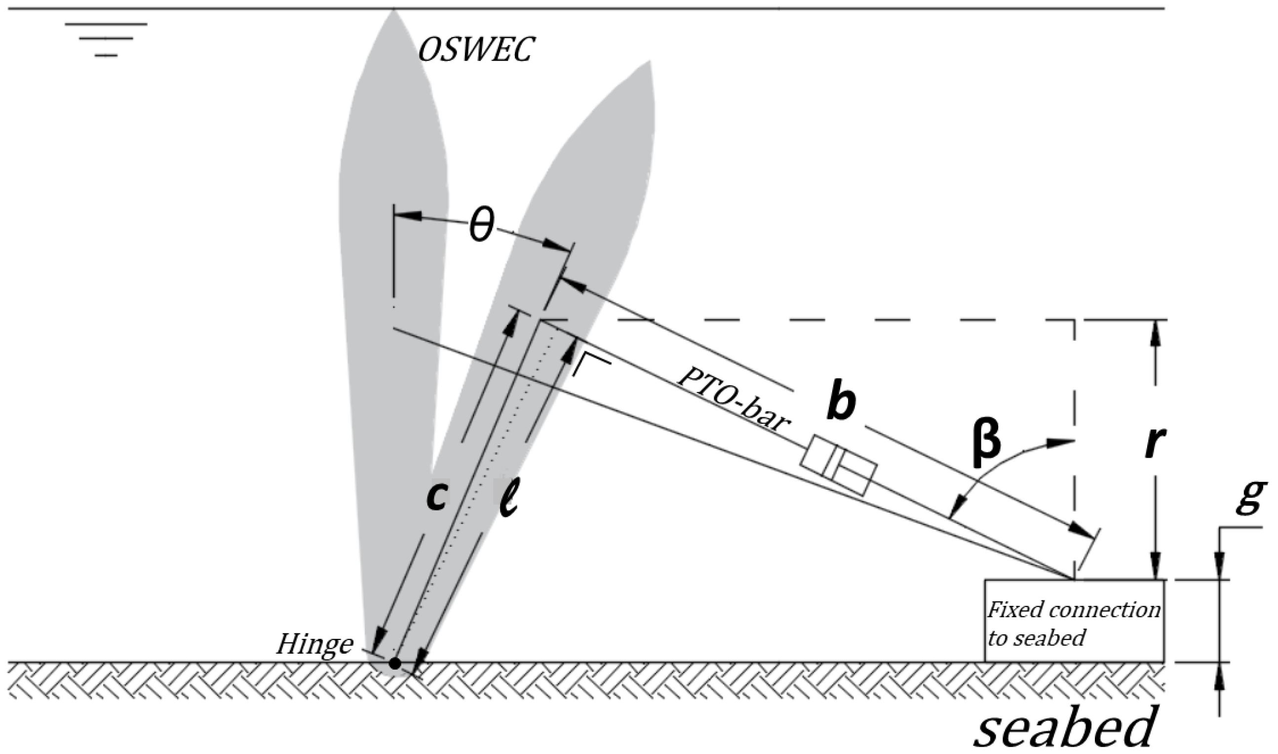
The Equation (23) is the absorbed power without taking into account losses in the hydraulic motor and electric generator. The average electrical power will be less than the power at the piston, $P_h$, since friction in the hydraulic motor and the efficiency of the generator are taken into account in WEC-Sim. In Section 4.4 and further, only the average absorbed power at the piston $P_h$ will be considered. WEC-Sim also provides the ability to implement a hydraulic PTO system for an OSWEC. The principle of a hydraulic PTO system applied to a pitching flap is sketched in Figure 2. In Figure 2, a positive pitching angle $\theta$ corresponds to a clockwise movement of the flap, which implies a shortening of the PTO-bar equipped with the PTO system. This shortening in its turn creates a pressure difference on both sides of the piston. The pitching motion thus induces a linear movement in the piston. Once this linear motion is calculated in Simulink, the force $f_{PTO}$ can be calculated and will be multiplied with the lever arm length ℓ around the hinge to find the torque ${\mathcal{T}}_{PTO}$:

$${\mathcal{T}}_{PTO}\left(t\right)=f_{PTO}\left(t\right)·\ell \left(t\right).$$

(24)

How the force $f_{PTO}$ is calculated is explained in Section 3.1.2, in Equation (15), since the hydraulic PTO system for the OSWEC mainly contains the same components as the one for the heaving cylindrical WEC. How the pitching motion of the flap is converted in a linear movement of the piston is briefly explained below. This conversion involves some geometric parameters—see Figure 2 for definitions:

• $\theta \left(t\right)$, the varying pitch angle
• g, the offset height of the PTO-bar connection with the seabed
• c, the distance between the flap-hinge and connection with the PTO-bar
• $b\left(t\right)$, the length of the PTO-bar, varying in time; for $\theta =0$, $b=b_{ini}$
• $r\left(t\right)$, the vertical distance between the connection points of the PTO-bar, varying in time
• $\beta \left(t\right)$, the angle between the PTO-bar and the vertical direction, varying in time
• $\ell \left(t\right)$, the length of the lever arm (or the distance of the hinge to the PTO-bar), variable in time.

In Figure 2 the length r varies in time and is evaluated by $r\left(t\right)=c·\cos \left(\theta \right(t\left)\right)-g$, while angle $\beta \left(t\right)$ can be calculated as $\beta \left(t\right)=\arccos \left(r\right(t)/b(t\left)\right)$. The length of the lever arm ℓ, i.e., the perpendicular distance from the PTO-bar to the hinge can be determined using:

$$\ell \left(t\right)=\sin \left(\theta \right(t)+\beta (t\left)\right)·c$$

(25)

The instantaneous absorbed power can be either determined by multiplying ${\mathcal{T}}_{PTO}$ with the angular velocity $\dot{\theta }$ or by multiplying $f_{PTO}$ with the linear velocity of the piston at each time step, as in Equation (23). As with the heaving cylindrical WEC, only the total absorbed power $P_h$ at the piston will be considered. The average absorbed power by the hydraulic PTO system of an OSWEC over one wave period is expressed as:

$$P_h=-\frac{1}{T}{\int }_0^T{\mathcal{T}}_{PTO}\left(t\right)·\dot{\theta }\left(t\right)dt$$

(26)

4. Modelled WECs and Input Wave Conditions

In this paper, we present the results for full scale WECs for a series of regular waves of varying heights and periods. The WEC types are outlined in Section 4.1 and the input wave conditions are shown in

Table 1. Test matrix of regular wave conditions.

Wave Height, H (m)	Wave Period, T (s)
1.0	6.0	8.0	10.0	12.0
2.0	6.0	8.0	10.0	12.0

in Section 4.2.

4.1. Modelled WEC Types

The two types of full-scale WECs modelled in this study are a heaving cylindrical buoy and a pitching bottom fixed flap, which is often termed OSWEC [34]. The heaving cylindrical WEC type is a flat cylinder with radius (r) of 10 m and a draft ($h_z$) of 2.0 m (see Figure 3). The shape was selected based on its overall dimensions being similar to several promising WEC technologies, namely that of Carnegie Wave [35] and SINN Power [36]. Moreover, as noted in a recent study, [37], such a flat disk shape provides a balance between the power absorption, WEC bandwidth, and material cost considerations. Please note that in our case the buoy is not fully submerged as in the case of the Carnegie CETO™ and is instead floating at equilibrium position with a draft of $h_z$ = 2.0 m. The natural or resonance period of the WEC in heave, $T_{r,33}\equiv 5.46$ s. The second is a bottom-fixed surface-piercing OSWEC with a width (w) of 20 m, a height (h) of 12 m, a draft ($h_z$) of 10 m, and a thickness ($\delta x$) of 1.0 m (see Figure 3). The OSWEC is similar to several pre-commercial WEC technologies, specifically the WaveRoller, developed by Finnish company AW-Energy. The natural pitch period of the OSWEC, $T_{r,55}\equiv 17$ s.

4.2. Input Wave Conditions

To demonstrate the utility of the presented PTO model coupling, regular waves of two wave heights and four wave periods are simulated as shown in Table 1.

Each PTO system configuration presented in Section 4.1 and each WEC type in Section 4.1 is modelled for all wave conditions. In the following Section 4.3 and Section 4.4, we determine the optimal PTO system coefficient for each WEC and PTO system type for each wave condition defined in Table 1.

4.3. Optimal PTO System Coefficients: Linear PTO

In Section 3.1.1 it was stated that an optimal value exists for the linear PTO system damping coefficient $B_{PTO,l}$, resulting in the maximum average absorbed power. These damping coefficients are first calculated for the specific case of the heaving cylindrical WEC with Equation (11), for the dimensions described above. The theoretically found values are summarized in

Table 2. Optimal linear $B_{PTO}$ coefficients for a heaving cylindrical WEC (${10}^6\times$ kg/s) and OSWEC (${10}^6\times$ (kg· m${}^2$)/s).

T (s)	6	8	10	12
Heaving Cylindrical WEC	1.12	2.25	3.46	4.65
OSWEC	128.0	98.40	69.70	51.0

. To calculate the corresponding coefficients for the OSWEC, (13) is applied for the OSWEC with the prescribed dimensions of Figure 3. Results for the optimal linear PTO damping coefficients are given in Table 2.

4.4. Optimal PTO System Coefficients: Hydraulic PTO

4.4.1. Optimal Hydraulic PTO System Coefficients for a Heaving Cylindrical WEC

It was proven that an optimal linear damping coefficient exists when a linear PTO system is applied. Since the PTO-force of a hydraulic PTO system, $f_{PTO,h}$ is no longer linearly dependent on the velocity of the heaving cylindrical WEC, no straightforward relationship for an optimal configuration of the hydraulic PTO system can be expressed. To find optimal PTO system parameters, a similar approach as in [38] is followed: a hydraulic PTO system damping term $B_{PTO,h}$ is defined and it is checked for an optimum value. Note however that this damping coefficient $B_{PTO,h}$ cannot be used to calculate the PTO-force $f_{PTO,h}$ by multiplying $B_{PTO,h}$ with the WEC’s velocity. It is a coefficient that takes into account the different parameters of the hydraulic PTO system that influence the performance of the WEC, with the same dimensions as the linear damping term $B_{PTO,l}$ [kg/s]:

$$B_{PTO,h}={\left(\frac{s_c}{D_m}\right)}^2{B}_g$$

(27)

$B_{PTO,h}$ can be changed by modifying the piston area, $s_c$, the motor displacement, $D_m$ or the generator damping, $B_g$, see Figure 1. In practice it is most convenient to alter the motor displacement $D_m$ [38], e.g., by installing a variable displacement motor as hydraulic motor. It is assumed that the swashplate angle $\alpha$ equals one. Since only $D_m$ will be varied in the following procedure, it is assumed that $s_c$ and $B_g$ are constant: $s_c$ is set as 0.0707 m${}^2$ and $B_g$ as 6 $\frac{\mathrm{Nm}}{\mathrm{rad}/\mathrm{s}}$, respectively, based on a prior analysis. Figure 4 proves the existence of an optimal value for $B_{PTO,h}$ for different wave periods in regular waves. As with the linear PTO system, the optimal value for $B_{PTO,h}$ increases with increasing wave period T. Due to the inherent non-linearities of the hydraulic PTO system, a different optimal value for $B_{PTO,h}$ could be expected for a different wave height H at the same wave period T. However, only a small change was observed in the optimal value for $B_{PTO,h}$ when altering the wave height H from 1.0 m to 2.0 m. The same conclusion was made in [38]. Since the average absorbed power $P_h$ stays rather constant close to the optimal value for $B_{PTO,h}$, the effect of a small change in $B_{PTO,h}$ close to its optimum value on $P_h$ is negligible. Therefore, the $B_{PTO,h}$ coefficients summarized in

Table 3. Optimal hydraulic damping coefficients $B_{PTO,h}$ for a heaving cylindrical WEC (${10}^6\times$ kg/s) and OSWEC (${10}^6\times$ m${}^2·$ kg/s).

WEC Type	T (s)	6	8	10	12
Heaving Cylindrical WEC	H = 1.0 m	1.5	3.25	4.7	8.3
OSWEC	H = 1.0 m	275	175	121	95

will be used for both H = 1.0 m and for H = 2.0 m.

The optimal hydraulic PTO system damping coefficients for the heaving cylindrical WEC for the studied wave conditions are summarized in Table 3.

4.4.2. Optimal Hydraulic PTO System Coefficients for the OSWEC

Section 3.1.2 also described the application of a hydraulic PTO system to an OSWEC. As with the heaving cylindrical WEC, optimal hydraulic parameters will be found for the OSWEC with dimensions as given in Section 4.1. The piston area was set equal to $s_c$ = 0.1257 m${}^2$ while the generator damping $B_g$ is set to $10\frac{\mathrm{Nm}}{\mathrm{rad}/\mathrm{s}}$, both values resulting from a prior analysis. Please note that additional geometric parameters must be considered when studying the optimal configuration for an OSWEC with a hydraulic PTO system—see Section 3.1.2 and Figure 2. The hydraulic PTO system applied to the OSWEC exerts a torque, ${\mathcal{T}}_{PTO}\left(t\right)=f_{PTO}\left(t\right)·\ell \left(t\right)$, depending on the PTO-force $f_{PTO}$ and the lever arm ℓ, calculated as in Equation (25). The latter depends on the following geometric parameters: g, c and b as defined in Figure 2. This implies that, contrary to the case of the heaving cylindrical WEC, not only the characteristics of the hydraulic PTO system, but also the initial geometric parameters g, c and $b_{ini}$ must be chosen carefully. The reasoning followed in the procedure of optimizing the hydraulic PTO system will briefly be explained below. It is firstly assumed that an optimal PTO-torque exists for each wave period, ${\mathcal{T}}_{PTO,opt}$. When then e.g., c increases, ℓ will increase as well, keeping all other parameters constant. This will result in a lower $f_{PTO,opt}$ to achieve the same ${\mathcal{T}}_{PTO,opt}$. $f_{PTO}$ can be lowered by increasing $D_m$. Changing the motor displacement will result in a different pressure difference between the accumulators and a different motor speed. The geometric configuration of the hydraulic PTO system for the OSWEC can thus be chosen in such a way that allows the most convenient hydraulic motor parameters. It may be expedient to limit the motor speed or the pressure difference to a certain value, which can be realized by adapting the motor displacement accordingly. A brief numerical analysis has shown that higher values for c and thus higher motor optimal displacements $D_m$ result in lower pressure differences. However, this distance c will probably have to be limited as well due to practical considerations. When looking at sketches of the WaveRoller OSWEC, the hydraulic PTO system seems to be very close to the seabed. After a brief analysis, it was chosen to put c equal to 3.0 m, g to 1.5 m and $b_{ini}$ to 5.0 m. $D_m$ was varied to find an optimal value that results in the maximum $P_h$. To express an equivalent $B_{PTO,h}$ for the OSWEC (similarly as was done for the heaving cylindrical WEC), following formula is used, resulting in a coefficient with the same dimensions as the linear damping term for the OSWEC:

$$B_{PTO,h}=c·b_{ini}{(\frac{s_c}{D_m})}^2{B}_g.$$

(28)

Figure 5 shows the average absorbed power $P_h$ for different values of $B_{PTO,h}$ for the four considered wave periods described in Section 5.2 and a wave height H = 1.0 m. The optimal value for $B_{PTO,h}$ decreases with increasing wave period, for this range of wave periods. The same conclusion was made for the OSWEC with a linear PTO system: the optimal value for $B_{PTO,l}$ decreases with increasing wave period.

5. Comparing the Effects of a Linear to a Hydraulic PTO System for a Single Heaving Cylindrical WEC and a Single OSWEC

5.1. Comparing the Average Power Output for Each WEC vs. Type of PTO System

The average power output for a single WEC of each type is calculated via Equation (10) or Equation (14) for the linear PTO system and via Equation (23) or (26) for the hydraulic PTO system. Please note that for the latter PTO system type the losses in the generator will not be taken into account to provide a fair comparison with the linear results, as noted in Section 3.1.2. The $B_{PTO}$ settings used are described in Section 4.3 and Section 4.4. Results for the modelled wave conditions of Table 1 are shown in

Table 4. Average power output for a single WEC for a linear and hydraulic PTO system. Heaving cylindrical WEC: top two rows. OSWEC: bottom two rows.

WEC Type	Wave Height H (m)	Average Power Output Linear ${\mathit{P}}_{\mathit{l}}$ (kW)				Average Power Output Hydraulic ${\mathit{P}}_{\mathit{h}}$ (kW)
		Wave Period T (s)				Wave Period T (s)
		6.0	8.0	10.0	12.0	6.0	8.0	10.0	12.0
heaving cylindrical WEC	1.0	47.98	65.94	72.86	72.04	50.15	77.40	90.05	85.34
	2.0	191.91	263.78	291.46	288.14	200.61	311.36	364.59	344.15
OSWEC	1.0	106.47	132.75	131.55	126.83	92.56	114.34	113.08	109.43
	2.0	425.87	531.03	526.49	508.78	367.98	452.59	447.95	434.39

. We note that the results for H = 2.0 m are almost exactly 4 times the results for H = 1.0 m, indicating that the non-linear influence of the hydraulic PTO system in these operational wave conditions is minimal. Therefore, we will focus on the results for a H = 1.0 m wave, which we plot in the bar chart in Figure 6.

$$\frac{P_h-P_l}{P_l}·100.$$

(29)

The percent difference is defined by Equation (29). We observe that for the heaving cylindrical WEC, the average power output is always greater with the hydraulic PTO system than with the linear PTO system while, in comparison, for the OSWEC the situation is reversed.

It can be seen that there is a notable increase in the average power output for the hydraulic PTO system ($P_h$) versus the linear ($P_l$) for the case of the heaving cylindrical WEC for periods $T\ge 8.0$ s. For these wave conditions, the hydraulic PTO system can damp the motion of the WEC to match the phase of the incident wave condition more effectively. Such is not the case with the OSWEC, where the natural pitching period of the WEC is higher than the investigated wave periods and the hydraulic PTO system is not performing optimally, i.e., it cannot ‘speed up’ the relative motion. We must note, however, that the linear PTO system for the OSWEC, although it shows on average a 15% improvement in the power performance of the WEC, may be making unrealistic assumptions about the motion of the OSWEC that may result in an artificially increased average power output. Observe that in all cases the average power output for the OSWEC is much higher than for the heaving cylindrical WEC, indicating that the OSWEC is more efficient in absorbing the power of the incoming waves; how this power absorption affects the wave field will be explored in the next Section 5.2.

5.2. Analyzing the Wave Field around One WEC

5.2.1. Calculating the Total and Perturbed Wave Fields

To calculate the wave field around a single WEC for a wave height H, we sum the complex incident unidirectional regular wave field, calculated at each point via Equation (30)

$$\zeta (x,y)={\displaystyle \frac{H}{2}}{e}^{-i\left(kx\right)}$$

(30)

to the perturbed wave field consisting of the radiated and diffracted wave fields. Both are calculated from their respective potentials via the kinematic free surface boundary condition Equation (5). The radiated wave field is given by Equation (31)

$${\eta }_r=-\frac{ZH}{\zeta }{\displaystyle \frac{i\omega {\varphi }_r}{2g}}.$$

(31)

Here ${\varphi }_r$ is the radiated wave potential and the ratio of the body displacement Z to the wave amplitude $\zeta$ is the response amplitude operator (RAO) which is calculated in Equation (32):

$$\frac{Z}{\zeta }=\frac{F_e}{-{\omega }^2{(M+A)}^2-i\omega (B_{PTO}+B)+K}$$

(32)

The modulus of the complex RAO calculated in Equation (32) is the amplitude of the WEC’s position divided by the wave amplitude:

$$|RAO|=|{\displaystyle \frac{Z}{\zeta }}|$$

(33)

Equation (32) is only valid when modelling a WEC with a linear PTO system. In Equation (32) $F_e$ is the excitation force, M the mass of the device, and $A,B$ and K, the added mass, hydrodynamic damping, and hydrodynamic spring or stiffness coefficients, respectively, determined in NEMOH for each of the relevant degrees of freedom. The $B_{PTO}$ is the linear $B_{PTO,l}$ coefficient in Table 2 for each wave period and WEC type. It is important to mention that the use of the hydraulic PTO coefficient $B_{PTO,h}$, as described in Section 4.4.1 and Section 4.4.2, in Equation (32) will lead to incorrect results. The coefficient $B_{PTO,h}$ was composed to combine all significant factors influencing the average absorbed power $P_h$, to check if an optimum value of the average absorbed power exists and to study the trend of this coefficient over a range of periods. Since the RAO for a WEC with a hydraulic PTO system cannot be calculated analytically, this RAO is determined using numerical time-domain simulations. For a given wave period and wave height, the WEC’s displacement is calculated numerically using WEC-Sim. The modulus of the RAO is calculated with Equation (33), whereas the RAO’s phase is determined as in Equation (34):

$$\phi =\omega ·\Delta t,$$

(34)

where $\Delta t$ represents the time shift between the WEC’s displacement profile and the surface elevation profile. Since the WEC’s position $z\left(t\right)$ is not sinusoidal when equipped with a hydraulic PTO system, the following method is used for the calculation of the time shift $\Delta t$:

$$\Delta t=\underset{\tau }{\mathrm{argmax}}{\int }_0^{T}z\left(t\right)·\zeta (t-\tau )dt.$$

(35)

The RAO phase $\phi$ will be positive since the WEC’s motion is delayed with respect to the incoming wave ($\Delta t$ > 0). The complex value of the RAO is now determined as:

$$\frac{Z}{\zeta }=|\frac{Z}{\zeta }|e^{i\phi }.$$

(36)

The diffracted wave amplitude ${\eta }_d$ is given by Equation (37)

$${\eta }_d=-{\displaystyle \frac{i\omega {\varphi }_{d}H}{g}},$$

(37)

where ${\varphi }_d$ is the diffracted wave potential. We calculate the wave field around a single WEC for each of the incident wave conditions presented in Table 1. In the two sections following, Section 5.2.2 and Section 5.2.3, we show representative results from the 24 cases simulated. Please note that the tally takes into account the fact that for the linear PTO system the result for H = 1.0 m and H = 2.0 m are the same.

5.2.2. The Influence of the WEC Type on the Wave Field

Before diving into the complicated patterns seen in the ‘near-field’ $\eta$ of the array, we model a single WEC in the numerical domain to clarify the impact of WEC type and PTO system type on the wave field. The two WEC types presented in Section 4.1 have a substantially different impact on the incoming waves as witnessed in the plots of the modulus of total wave field $|\eta |$, in Figure 7 for one heaving cylindrical WEC (left) and an OSWEC (right) for a linear PTO system for the same incident wave of H = 1.0 m and T = 6.0 s. The total $|\eta |$ is the modulus of sum of the complex perturbed $\overline{\eta }$ and the complex incident wave $\overline{\eta }$. We see right away that the perturbation effect for the OSWEC is much greater than that of the heaving cylindrical WEC, both in magnitude and extent away from the WEC. This difference is largely a consequence of the diffraction potential of the OSWEC since it presents a barrier to the entire water column compared to the small-draft heaving WEC which presents much less resistance to the incoming waves. As an example, we can observe this difference in Figure 8 for a H = 1.0 m, T = 10.0 s wave where the diffraction is plotted for a heaving cylindrical WEC on the left and for an OSWEC on the right.

Moreover, the difference in the radiated wave field is significant as well, especially as we move to higher wave periods, where the OSWEC responds more to the incoming wave whereas the heaving cylindrical WEC is essentially riding on top of the water column. This is significant in our study because it is indeed the radiation which we can influence throughout the PTO model as will be witnessed in the next subsection.

5.2.3. The Influence of the PTO System Type on the Wave Field for a Single WEC

As mentioned in the previous paragraph in Section 5.2.2, the discrepancy between the radiation of the two WECs is less than the difference in diffraction for a given wave. However, it is still significant, and as the radiated wave field is a function of the PTO system as well as the WEC type, we do see a divergence in the perturbed wave field between the different PTO system types. This is noted in a plot of the percent difference between the total $|\eta |$ for the linear and the hydraulic PTO system first for the heaving cylindrical WEC (left) and the OSWEC (right) in Figure 9 for a H = 1.0 m, T = 8.0 s wave.

We observe that the variability between the two PTO system types is less than 5 % for the heaving cylindrical WEC while that for the OSWEC is closer to 10 % in the region near the device. This is not demonstrated in the results in the power output (P) however, where in Table 4 in Section 5.1 for the H = 1.0 m, T = 8.0 s wave, the difference between $P_l$ and $P_h$ is 17% and only 14% for the OSWEC. Moreover, $P_h-P_l$ is positive for the heaving cylindrical WEC while the addition of a hydraulic PTO system actually reduces the power output for an OSWEC. This situation is mirrored for the other wave periods where the increase in the perturbed wave field for the OSWEC compared to that of the heaving cylindrical WEC does not induce an increase in the power output of the OSWEC $P_h$.

6. Analyzing the Power Production and the Near-Field Effects for an Array of 5 WECs With a Hydraulic PTO System

6.1. WEC Array Layout

As we have seen in the results for a single WEC in Section 5, the perturbed wave field around a single WEC strongly depends on both the WEC type and the PTO system modelled. In this section, we extend our results to an array of 5 WECs with a view toward the modelling of a commercial scale WEC farm consisting of multiple WEC arrays. To this end we model two different 5-WEC arrays: one consisting of heaving cylindrical WECs (Figure 10) and the other of pitching OSWECs (Figure 11). The WEC-WEC separation distances $d_x$ and $d_y$ are set to 40 m, which is the $2\times$ the diameter of the heaving buoy WEC and the width of the OSWEC. The array configurations of both WEC types are staggered, an arrangement that was clearly shown to be power-maximizing in several numerical and experimental studies such as in [4,23,26,28,39,40,41]. In this investigation the water depth is set at 30 m for the heaving buoy and 10.0 m for the OSWEC.

6.2. 1st Order Approximation for the WEC Array Near-Field

To assess the effects of multiple WECs in a WEC array or multiple WEC arrays in a WEC farm on the power output ($\mathbf{P}$) of the farm, we need to calculate the total perturbed wave field in the near-field domain. As we assume linear theory in our work, we can use the superposition principle to sum up the total wave field by using an iterative approach first developed in [42]. The technique employed is illustrated in Figure 12. The initial step (Step 1) is to propagate the incident wave in the empty numerical basin (no WEC present) to obtain the undisturbed surface elevation. In Step 2 the incident surface elevation is used as input into NEMOH whence the 1st order perturbed wave of WEC Array I, $p_{1i}$, is evaluated. In Step 3, the average wave amplitude at the location of $p_{1i}$ is used as input into NEMOH to calculate the 1st order perturbed wave of WEC Array II, $p_{1ii}$. In Step 4, the process in Step 2 is repeated, with $p_{1ii}$ as the new input perturbed wave. Finally, in Step 5, the same process is performed for the 2nd perturbed wave of WEC Array I, $p_{2i}$. Since the input perturbed wave in each subsequent step after step is reduced by approximately an order of magnitude, for all practical purposes this process can be terminated at Step 4 without any appreciable loss in accuracy, even for the case where interaction is maximized. Therefore, Step 5 is only displayed for a complete description of the proposed iterative method. To calculate the perturbed $\eta$, in this paper we limit the summation to the 1st order perturbed waves from each WEC in the array. The power for each WEC is calculated using the average surface elevation that is the sum of the incident wave and the perturbed waves from the nearest two WECs.

6.3. Power Output Calculation for an Array of 5 WECs

In evaluating the influence of the 5-WEC array interaction effects on the performance of a wave farm, we compute the total power output by the two WEC arrays, after having obtained the modified wave field in the WEC array using the approach outlined in Section 6.2. The power of each array is calculated by the following equations depending on the PTO system and WEC type. For the linear PTO system, we extend Equations (10) and (14) to $\mathcal{M}$ WECs operating in one DoF to Equation (38),

$$\begin{array}{c}\hfill {\mathbf{P}}_l=-\frac{1}{2}{\mathbf{B}}_{PTO,l}{|\mathbf{Z}\left(\omega \right)|}^2{\omega }^2,\end{array}$$

(38a)

$$\begin{array}{c}\hfill {\mathbf{P}}_l=-\frac{1}{2}{\mathbf{B}}_{PTO,l}{|\theta \left(\omega \right)|}^2{\omega }^2,\end{array}$$

(38b)

where $\mathbf{Z}$ and $\mathbf{\theta }$ indicate an $\mathcal{M}\times 1$ column vector of the WEC’s position or angular displacement, respectively. ${\mathbf{B}}_{PTO,l}$ represents an $\mathcal{M}\times \mathcal{M}$ diagonal matrix with the $B_{PTO}$ coefficients for each WEC on the diagonal. For the hydraulic PTO system, the equations equivalent to (23) and (26) are given in Equation (39):

$$\begin{array}{c}\hfill {\mathbf{P}}_h=-\frac{1}{T}{\int }_0^T{\mathbf{F}}_{PTO}\left(t\right)·\dot{\mathbf{z}}\left(t\right)dt,\end{array}$$

(39a)

$$\begin{array}{c}\hfill {\mathbf{P}}_h=-\frac{1}{T}{\int }_0^T{\mathcal{T}}_{PTO}\left(t\right)·\dot{\mathbf{\theta }}\left(t\right)dt.\end{array}$$

(39b)

Here as in Equation (38), the boldface quantities represent $\mathcal{M}\times 1$ column vectors of the forces and velocities of the individual heaving cylindrical WECs of the torques and angular displacements of the individual OSWECs. As mentioned in Section 6.2, for each WEC in the array, the motions and the forces used in Equations (38) and (39) are calculated with the input wave equal to the incident wave plus the 1st order WEC array perturbed wave at the location of the given WEC. The magnitude of the $\eta$ used for calculating the power $\mathbf{P}$ in Equations (38) and (39) is taken as the average of the 1st order modified $\eta$ on a region immediately surrounding the WEC. In addition to calculating the power of each array, we also introduce the ‘q value’, defined as the ratio of the power of the $\mathcal{M}$-WEC array to the power produced by the sum of $\mathcal{M}$ WECs as if they were operating in isolation:

$$q={\displaystyle \frac{{\mathbf{P}}_{Array}}{\sum P}}.$$

(40)

where P is the power output of the linear or hydraulic PTO WEC given by equations (Equations (10), (14), (23) and (26)) for the heaving cylindrical WEC or the OSWEC, respectively. The q value is a commonly used metric in wave energy literature to assess the strength of array effects, we find it used in [30,39,40,43], for example.

6.4. Power Output for an Array of 5 WECs

The 5-WEC array power output for the two PTOs and for the data for the two WEC types is displayed in

Table 5. Average power output for an array of 5 WECs for a linear and hydraulic PTO system. heaving cylindrical WEC: top three rows. OSWEC: bottom three rows.

WEC Type	Value	Wave Height H (m)	Average Power Output Linear ${\mathit{P}}_{\mathit{l}}$				Average Power Output Hydraulic ${\mathit{P}}_{\mathit{h}}$
			Wave Period T (s)				Wave Period T (s)
			6	8	10	12	6	8	10	12
heaving cylindrical WEC	ARRAY	H = 1.0	234.54	325.48	315.33	304.44	245.7	387.28	389.27	358.25
	SINGLE × 5	H = 1.0	239.9	329.72	364.32	360.18	250.77	386.99	450.26	426.69
	q	H = 1.0	0.98	0.99	0.87	0.85	0.98	1.00	0.86	0.84
OSWEC	ARRAY	H = 1.0	1001.7	1736.6	1282.6	854.33	867	1617.7	1237.8	868.79
	SINGLE × 5	H = 1.0	532.34	663.75	657.75	634.15	462.8	571.7	565.4	547.2
	q	H = 1.0	1.88	2.62	1.95	1.35	1.87	2.83	2.19	1.59

for the modelled wave periods from Table 1 for H = 1.0 m and in the bar chart Figure 13. The q value for the various configurations, defined in Equation (40), is displayed in the third and sixth data row. As we have witnessed in Section 5.1, the deviation from linear behavior due to the increase from H = 1.0 m to H = 2.0 m is very small, therefore we will focus our attention in this and the following sections on the results for H = 1.0 m with the knowledge that the results for H = 2.0 m show similar patterns and behaviors. As in the single WEC case, we observe a significant increase in the power output of the 5-OSWEC array versus a 5-heaving cylindrical WEC array with the power of the former producing up to 3× more power for a wave period of 8.0 s. Please note that as in the single WEC case analyzed in Section 5.1, the heaving cylindrical WEC array produces more power with increasing wave period while in the case of the OSWEC array, the peak power occurs for T = 8.0 s, with a decrease for higher wave periods. Please note that this reduction is more significant in the array case than in the single wave case, a fact that is reflected in the decreasing q values as the period increases. This behavior can be directly linked to the increase in the $|\eta |$ in the ‘near-field’ zone, as we will observe in Section 6.5.2. For the heaving cylindrical WEC, the q values are also decreasing for wave periods greater than 8.0 s, but with the difference that each q value is consistently below unity. It is clear from the data that in the case of the modelled 5-WEC array configuration, placing the OSWECs in an array is much more advantageous to their performance than for the heaving cylindrical WECs. We must remark however, that in realistic wave conditions with frequency and directional spreading it is near impossible to achieve the phase relationships that lead to high q values and consequently, we expect the relative difference in the array power output between the two types of WECs to diminish.

6.5. The Near-Field $|\eta |$ for an Array of 5 WECs

In this section, we present the results for the near-field wave field for an array of 5 heaving cylindrical WECs, arranged in the configurations displayed in Figure 10 and Figure 11 for the wave periods listed in Table 1 for a wave height H of 1.0 m. The results are presented in Section 6.5.1 and Section 6.5.2 as the modulus of the surface elevation $|\eta |$. Using this metric, we show both the total wave field to see the connection between the surface elevation and the array power output, and the perturbed wave field which only displays the array effects, that is deviations from the incident wave field brought about by the interactions with the WEC arrays. Because of the quantitative differences in the wave fields for a heaving cylindrical WEC and an OSWEC, the presentation of the results is split into two Section 6.5.1 and Section 6.5.2, where in each subsection we take an in-depth look at the ‘near-field’ wave amplitude $\eta$.

6.5.1. The Perturbed $|\eta |$ for an Array of Heaving Cylindrical WECs

First thing, we look at the wave field of an array of 5 heaving cylindrical WECs for a linear PTO system for T = 6.0 s and T = 8.0 s. In Figure 14 and Figure 15 the total (left) and perturbed (right) fields are plotted for the named wave periods. Notice that the magnitude of the changes in the total $|\eta |$ due to the presence of the array are much greater for the case of T = 6.0 s. This can be seen even more clearly in a comparison of the perturbed $|\eta |$ for the same two wave periods, where the perturbed wave field is nearly 2× greater in magnitude near the WECs. However, it would be incorrect to assume that this difference is linearly proportional to the difference in the power output $\mathbf{P}$ of the array at these wave periods, as will be elaborated on in Section 7.

Moving on to the two higher wave periods, T = 10.0 s and T = 12.0 s, the interaction of the incident wave field with the WEC array markedly decreases. We can observe this in a contour plot of the total and the perturbed wave field for T = 10.0 s for the heaving cylindrical WEC array with a linear PTO system in Figure 16. We note that although the perturbed wave field is barely perceptible, it does result in a slight enhancement of the total wave field which creates an area of higher total $|\eta |$ in front of the array. For T = 12.0 s the shape of the interaction zones is similar to those of T = 10.0 s but the magnitude of the array effects is minimal and consequently, these wave fields are not displayed in the interest of brevity.

6.5.2. Results for an Array of OSWECs

We next move on to explore the results of the simulations for the 5-OSWEC Array. Analogous to Section 6.5.1 we first look at the total near-field $|\eta |$ for T = 6.0 s and T = 8.0 s, which are the wave periods with the greatest ‘array effect’ and the highest power output $\mathbf{P}$. In Figure 17 and Figure 18 we plot the total $|\eta |$ (left) and the perturbed $|\eta |$ for the two wave periods in question. Observe that the magnitude of both fields is much greater than that of the heaving cylindrical WEC shown in Figure 14 and Figure 15 for both T = 6.0 s and T = 8.0 s. Moreover, we observe a large difference in the locations of ‘hot spots’ and ‘cold spots’, which are areas of strong positive or negative anomalies in $|\eta |$ between T = 6.0 s and T = 8.0 s. In other words, the areas with destructive interference between the incident and the perturbed wave leads to a decrease in $|\eta |$ or vice versa with constructive interference between the incident and perturbed waves. This is important in understanding the interaction between the wave period and the power output $\mathit{P}$ that we will discuss in Section 7.

As with the heaving cylindrical WEC, the two largest wave periods T = 10.0 s and T = 12.0 s display smaller perturbations in the near-field zone. Unlike for the heaving cylindrical WEC, however, they are still significant, as we can witness in Figure 19 and Figure 20 in the plots of the $|\eta |$ for an OSWEC with a linear PTO system. This perturbation effect is mirrored in the positive q values in Table 5 for both T = 10 and T = 12, unlike in the case of the heaving cylindrical WECs. Again, notice the strong change in the locations of the positive and negative anomalies in the total wave field between Figure 19 and Figure 20. As we will see in the next section Section 6.5.3, these are the two wave periods where the hydraulic PTO system power performance in a OSWEC array is close to or slightly exceeding the linear PTO system WEC array case, unlike the single WEC case in Section 5.1 where the reverse is true.

6.5.3. Comparing the Effect of a Linear PTO System to a Hydraulic PTO System for a Wave Field around a 5-WEC Array

In this section, we compare the effect of the linear and hydraulic PTO system on the near-field of the array. As in Section 6.5.1 and Section 6.5.2, we show the outcomes for both the total and perturbed wave fields, but instead of plotting $|\eta |$, we plot the percent difference between the $|\eta |$ of the WEC with hydraulic and the linear PTO system similar to Figure 9 for the a single WEC. We start by looking at the effect of the hydraulic PTO system for the case of the heaving cylindrical WEC. In Figure 21 we plot the difference between the total $|\eta |$ for a heaving cylindrical WEC for the 4 modelled wave periods as defined by Equation (29).

The first observation we make is the marked decrease in the $\eta$ difference as we increase T from 6.0 s to 12.0 s. While for the 6.0 s wave the difference barely exceeds 15 % for areas on the perimeter of the body, for the rest of the wave periods the differences are considerably less, dipping below the 5% threshold of the T = 12.0 s case. Please note that whereas for the two shorter wave periods the areas of positive and negative change have a complicated pattern based on the interaction between the radiated waves of each body, for the T = 10.0 s and T = 12.0 s cases there is a general trend of a higher $|\eta |$ for the hydraulic PTO system for the front rows and lower for the back row, especially for the back middle WEC. Observe that this slight overall decrease in $|\eta |$ does not adversely affect the heaving cylindrical WEC array performance, as we saw in Table 5 in Section 6.4, where the performance of the heaving cylindrical WEC array is significantly better than that of the single WECs.

Contrary to the heaving cylindrical WEC array, the difference of the PTO system greatly modifies the wave field of the 5-OSWEC array. In comparing Figure 22 to Figure 21, we see that the percent difference is much greater, in fact more than 100% for the 8.0 s case. We also observe that, unlike for the heaving cylindrical WEC array example, the differences in $|\eta |$ do not markedly decrease with increasing wave period. We see that difference is the greatest for T = 8 s but that it is also greater for T = 12.0 s than for T = 10.0 s. What we see then is that there is a strong effect the hydraulic PTO system on the WEC array wave field, and by comparing the contour plots in Figure 22 to the values for the average absorbed power of the OSWEC array in Table 5, we also notice that the difference in $|\eta |$ is not always proportional to the difference in power. For example, we notice that the magnitude and extent of the positive anomalies for T = 12.0 s is greater than that for T = 10.0 s but that the hydraulic PTO system 5-OSWEC array produces less power for the higher period. In general, we see that the difference from linear to hydraulic PTO system has a strong effect on the total wave field, but that the quality of the difference is greatly dependent on the wave period. We note that for the T = 8.0 s case in particular, there is an overall reduction in the surface elevation in lee of the array for the hydraulic PTO system compared to the linear PTO system, a fact that is reflected in the increase of the q value from 2.62 to 2.83. We can also observe that for the T = 10.0 s and especially the T = 12.0 s case that there is a net increase in $|\eta |$ inside the array area and a slight decrease outside of it. Again, we see this confirmed in the q values in Table 5 where they increment from 1.95 to 2.19 for the T = 10.0 s and from 1.35 to 1.59 for the T = 12.0 s wave.

7. Discussion

In the results for the 5-WEC arrays in Section 6 we have seen the interplay between the efficacy of the WEC array from the point of view of average absorbed power and the array wave fields $\eta$. The primary determination we can make is that the array effects are much stronger for the 5-OSWEC array case than for the heaving cylindrical WEC array case. Consequently, the effect of the change of the PTO system on the near-field surface elevations is much more significant for the OSWEC than for the heaving cylindrical WEC as highlighted in Figure 21 and Figure 22 in Section 6.5.3. As remarked in Section 6.4 in Figure 13, the effect of the change in PTO on the power output of the array is likewise quite different between the 5-heaving cylindrical WEC array and the 5-OSWEC array, but is not strictly related to the change in the magnitude of the array effects. The addition of a hydraulic PTO significantly increases the power output of the heaving WEC array, especially at the higher wave periods. Meanwhile for the OSWEC array, there is a net decrease in the array power output with a change from a linear to a hydraulic PTO system for all periods except for T = 12 s. The interplay between the impact of the PTO systems of the two WEC types placed a closely spaced WEC array on the array power and on the near-field $\eta$ are conceptualized in the flow chart in Figure 23. The arrow thickness represents the relative magnitude of the effect of each PTO type on the phenomena where the arrows are directed.

As with the magnitude, the location of the greatest changes in the near-field $\eta$ differs between the 5-heaving cylindrical WEC and the 5-OSWEC array. Observe that the areas of positive and negative % difference in $\eta$ are very distinct, with the hydraulic PTO system increasing the apparent $\eta$ behind the heaving cylindrical WEC array while for the OSWEC array the change from a linear to a hydraulic PTO reduces the $\eta$ behind the WECs. This is not a surprise given that the OSWEC, which operates in shallow water and fills the entire wave column, presents a bigger obstacle to the oncoming waves that results in much greater wave diffraction as observed in Figure 9. It is also the case that the OSWEC produces a stronger radiated wave field. The sum of the two effects results in strong areas of constructive and destructive interference that we observe in the surface elevations in the single OSWEC case in Figure 7 (left) and in the array of 5 OSWECs in Figure 17, Figure 18, Figure 19 and Figure 20. Note especially the enhancement in the wave fields for T = 8.0 s for the OSWEC where the perturbed field is up to 50 % greater around the bodies. This is manifested in the power output $\mathbf{P}$ of the 5-OSWEC array at this wave period in Table 5: $\mathbf{P}$ is the highest value among all wave periods for the OSWEC and also with the highest q value, for both PTOs. In contrast, the perturbed wave field for the heaving cylindrical WEC for T = 8.0 s is quite small, only differing by a few centimeters from the undisturbed $|\eta |$ as we see in the right panel in Figure 15. Moreover, the impact of the change in the PTO system of the heaving cylindrical WEC is not necessarily reflected in the power output of the heaving cylindrical WEC array. As an example, the 5-heaving cylindrical WEC array outputs the most power at a wave period of T = 8.0 s for a linear PTO system, for a hydraulic PTO system the power is higher for wave period of T = 10.0 s. Since the near-field array effects and the power output of a 5-heaving cylindrical WEC array are not directly linked, these changes are not reflected in Figure 21 where we see a relative decrease in the near-field $|\eta |$ between the case of a wave period of T = 8 s and T = 10 s.

When we observe the areas of positive or negative change based on a substitution of a linear for a hydraulic PTO system, in Figure 21, we note a decrease in the change in $\eta$ for the higher wave periods, indicating that the hydraulic PTO system is indeed extracting more energy from the wave field than the linear PTO system. However, the magnitude of these effects is close to the 5% threshold and can essentially be neglected in a 1st order modelling approach. Conversely, we have noted in Section 6.5.3 that the addition of a hydraulic PTO system to the OSWECs in an array tends to ‘pull’ in the energy from the surrounding areas to the ‘near field’. This is especially true for higher wave periods and is reflected in the relative increase in the power output of an OSWEC array with a hydraulic PTO system compared to the same isolated WEC. In the case of the OSWEC array, the effects are an order of magnitude stronger. We note the present results show the same differences in the strength of the array effects between the heaving cylindrical WEC and the OSWEC arrays as in those presented in [44].

We presume that such contrasting behavior reflects the differences in the underlying hydrodynamics of the WEC-PTO system of the 2 WEC types. For the heaving cylindrical WEC case, the primary driver of an increment in the power output of a hydraulic PTO system is the increase in the PTO system force, while for the OSWEC the hydraulic PTO system has a greater impact on the WEC motion. Indeed, the $\eta$ of near-field area of the OSWEC array increases with the hydraulic PTO system, especially for the long wave periods T = 10.0 s and T = 12.0 s. Unlike the heaving cylindrical WEC case, we also note that a change in the PTO system reduces the $\eta$ in lee of the WEC array, augmenting the areas of destructive interference. This might be important in considering the impact on surrounding WEC arrays and coastal processes.

Still, a change in PTO system for the OSWEC results in an improvement for only the T = 12.0 s, with a relative decrease in the power output for the other wave periods compared to the linear PTO system case. We must remark here that for the OSWEC case, for both the single WEC and the array, our linear PTO model can exaggerate the performance of the OSWEC since we are not taking into account the strong non-linearities inherent in the dynamics of this WEC type. This has been pointed out in [8,45] among others. Therefore, if we were to choose a more sophisticated model for the OSWEC, the relative ‘underperformance’ of the hydraulic PTO system might disappear.

It must be mentioned here that in this paper we are using a linear hydrodynamic model in simulating the WEC arrays for regular waves from a single direction. It has been shown in literature and in our own research that these assumptions would tend to overestimate both the power output and the perturbations in the near-field $\eta$. We note that a heaving cylindrical WEC, being axi-symmetric, is much less sensitive to changes in the direction of the incoming wave than the OSWEC. We also remark that for the case of the OSWEC, the linear PTO model might lead to an overestimation of the power and the differences we observe between a 5-OSWEC array power output with a linear and hydraulic PTO model might be in part be due to such assumptions. Therefore, we use the linear model more as a ‘benchmark’ to compare with previous studies such as [2,5,23,44] rather than a realistic PTO system representation to include in an OSWEC array simulation.

8. Conclusions

In this paper, we have presented a model of arrays of 5 WECs of two WEC types with contrasting hydrodynamics, a heaving cylinder WEC and an OSWEC driven by the surge component of the wave force. In our wave structure interaction-PTO model, we simulated single WECs and arrays with linear and hydraulic PTO systems, calculating both the power output of the WEC array and near-field $\eta$ of the WEC array using an original iterative method that enables a fast calculation of both quantities. We have elaborated on the distinct hydrodynamic behavior of the heaving cylindrical WEC and the OSWEC.

We noted the differing effects of changing of a WEC PTO system between a single WEC case and an array case as summarized by Figure 23. Pertaining to power output P for the single heaving cylindrical WEC case, we conclude that the hydraulic PTO system brings a significant increase in the power output compared to a linear PTO system with up to 25% improvement for a H = 1.0 m, T = 10.0 s wave. For an array of 5 heaving cylindrical WECs the result is similar, with the increase due to the hydraulic PTO system mirroring that of the single WEC case. In both cases the impact of the heaving cylindrical WEC array on the near-field is minimal, with the only significant modification of the wave field at a wave period of T = 6.0 s. By extension then, a change in the PTO type for a heaving cylindrical WEC array produces no substantial changes to the near-field surface elevations. Therefore, if these effects are the primary target of a given investigation, a hydraulic PTO system can be modelled as a linear PTO system without loss of fidelity.

Conversely, for a single OSWEC, a hydraulic PTO system tempers the performance, with a reduction in the power output P across all wave period around 14%. Intriguingly, the situation for a 5-OSWEC array is different, with the hydraulic PTO system only having a strong negative effect on power output for a T = 6.0 s wave. For the other wave periods the change in PTO system does not results in a decrease in the power output, indeed for T = 12.0 s it slightly increases. We can see, therefore, that for the case of a 5-OSWEC array the array effects play a strong role in modifying the WEC array power output. There is a two-fold conclusion then for modelling the OSWECs. Firstly, a single OSWEC with a specific PTO system cannot be expected to reflect the behavior of said PTO system in an array. Secondly, the difference between the two types of PTO systems modelled is great enough such that one cannot substitute one PTO system for another without introducing substantial error. As a practical consideration, most existing models of array PTO systems are simulated as linear PTO systems. Although a hydraulic PTO system is more difficult to model in practice, our results have shown that for the case of the OSWEC array with a hydraulic PTO system, it cannot be simplified down without introducing substantial error into both the array power output and the near-field effects. In both aforementioned cases, the WEC array modeler can use the conceptual schematic introduced in Figure 23 as a guideline for choosing which assumptions to make.

It is part of our ongoing research to gradually increase the complexity and sophistication of both the hydrodynamic and the PTO models with the counterbalance of having a fast and intuitive solution for WEC array modelling. It is the next step of our research to use the presented coupled models in a realistic WEC farm simulation using real sea states to test the limitations of the present research mentioned at the end of the discussion in Section 7. Furthermore, out research aim is to expand the calculation of the perturbed wave field to the ‘far-field’ area away from the WEC farms to study coastal effects and interactions with a changing bathymetry.

References

1. Venugopal, V.; Smith, G. Wave Climate Investigation for an Array of Wave Power Devices. In Proceedings of the 7th European Wave and Tidal Energy Conference, Porto, Portugal, 11–14 September 2007; p. 10. [Google Scholar]
2. Charrayre, F.; Peyrard, C.; Benoit, M.; Babarit, A. A Coupled Methodology for Wave-Body Interactions at the Scale of a Farm of Wave Energy Converters Including Irregular Bathymetry. In Proceedings of the ASME 2014 33rd International Conference on Ocean, Offshore and Arctic Engineering, San Francisco, CA, USA, 8–13 June 2014. [Google Scholar]
3. Göteman, M.; Engström, J.; Eriksson, M.; Isberg, J. Optimizing wave energy parks with over 1000 interacting point-absorbers using an approximate analytical method. Int. J. Mar. Energy 2015, 10, 113–126. [Google Scholar] [CrossRef] [Green Version]
4. Ruiz, P.M.; Ferri, F.; Kofoed, J.P. Experimental Validation of a Wave Energy Converter Array Hydrodynamics Tool. Sustainability 2017, 9, 115. [Google Scholar] [CrossRef]
5. Ruiz, P.M.; Nava, V.; Topper, M.B.R.; Minguela, P.R.; Ferri, F.; Kofoed, J.P. Layout Optimisation of Wave Energy Converter Arrays. Energies 2017, 10, 1262. [Google Scholar] [CrossRef]
6. Yu, Y.; Lawson, M.; Ruehl, K.; Michelen, C. Development and Demonstration of the WEC-Sim Wave Energy Converter Simulation Tool. In Proceedings of the 2nd Marine Energy Technology Symposium (METS 2014), Seattle, WA, USA, 15–17 April 2014. [Google Scholar]
7. Zhao, H.T.; Sun, Z.L.; Hao, C.L.; Shen, J.F. Numerical modeling on hydrodynamic performance of a bottom-hinged flap wave energy converter. China Ocean Eng. 2013, 27, 73–86. [Google Scholar] [CrossRef]
8. Schmitt, P.; Asmuth, H.; Elsäßer, B. Optimising power take-off of an oscillating wave surge converter using high fidelity numerical simulations. Int. J. Mar. Energy 2016, 16, 196–208. [Google Scholar] [CrossRef]
9. Henry, A.; Folley, M.; Whittaker, T. A conceptual model of the hydrodynamics of an oscillating wave surge converter. Renew. Energy 2017, 118, 965–972. [Google Scholar] [CrossRef]
10. Paredes, G.M.; Eskilsson, C.; Palm, J.; Bergdahl, L.; Leite, L.M.; Taveira-Pinto, F. Experimental and Numerical Modelling of a Moored, Generic Floating Wave Energy Converter. In Proceedings of the 10th European Wave and Tidal Energy Conference, Aalborg, DK, USA, 2–5 September 2013. [Google Scholar]
11. Schmitt, P.; Elsaesser, B. On the use of OpenFOAM to model oscillating wave surge converters. Ocean Eng. 2015, 108, 98–104. [Google Scholar] [CrossRef] [Green Version]
12. Devolder, B.; Rauwoens, P.; Troch, P. Numerical simulation of a single floating point absorber wave energy converter using OpenFOAM. In Proceedings of the 2nd International Conference on Renewable Energies Offshore, Lisbon, Portugal, 24–26 October 2016; pp. 197–205. [Google Scholar]
13. Verbrugghe, T.; Domínguez, J.M.; Crespo, A.J.; Altomare, C.; Stratigaki, V.; Troch, P.; Kortenhaus, A. Coupling methodology for smoothed particle hydrodynamics modelling of non-linear wave-structure interactions. Coast. Eng. 2018, 138, 184–198. [Google Scholar] [CrossRef]
14. Devolder, B.; Stratigaki, V.; Troch, P.; Rauwoens, P. CFD simulations of floating point absorber wave energy converter arrays subjected to regular waves. Energies 2018, 11, 641. [Google Scholar] [CrossRef]
15. Bharath, A. Numerical Analysis of Arrays of Wave Energy Converters. Ph.D. Thesis, University of Tasmania, Hobart, Australia, 2018. [Google Scholar]
16. Penalba, M.; Davidson, J.; Windt, C.; Ringwood, J.V. A high-fidelity wave-to-wire simulation platform for wave energy converters: Coupled numerical wave tank and power take-off models. Appl. Energy 2018, 226, 655–669. [Google Scholar] [CrossRef]
17. De, O.; Falcão, A.F. Phase control through load control of oscillating-body wave energy converters with hydraulic PTO system. Ocean Eng. 2008, 35, 358–366. [Google Scholar]
18. Folley, M.; Whittaker, T. The control of wave energy converters using active bipolar damping. J. Eng. Marit. Environ. 2009, 223, 479–487. [Google Scholar] [CrossRef]
19. Cargo, C.J.; Plummer, A.R.; Hillis, A.J.; Schlotter, M. Determination of optimal parameters for a hydraulic power take-off unit of a wave energy converter in regular waves. Proc. Inst. Mech. Eng. Part A J. Power Energy 2012, 226, 98–111. [Google Scholar] [CrossRef]
20. So, R.; Casey, S.; Kanner, S.; Simmons, A.; Brekken, T.K.A. PTO-Sim: Development of a power take off modeling tool for ocean wave energy conversion. In Proceedings of the 2015 IEEE Power Energy Society General Meeting, Denver, CO, USA, 26–30 July 2015; pp. 1–5. [Google Scholar] [CrossRef]
21. Sell, N.; Plummer, A.; Hillis, A.; Chandel, D. Modelling and calibration of a direct drive hydraulic PTO. In Proceedings of the Twelfth European Wave and Tidal Energy Conference, Cork, Ireland, 27 August–1 September 2017; pp. 886–1983. [Google Scholar]
22. Yu, Y.H.; Tom, N.; Jenne, D. Numerical Analysis on Hydraulic Power Take-Off for Wave Energy Converter and Power Smoothing Methods. In Proceedings of the 37th International Conference on Ocean, Offshore and Artic Engineering, Madrid, Spain, 17–22 June 2018; p. V010T09A043. [Google Scholar] [CrossRef]
23. Balitsky, P.; Verao Fernandez, G.; Stratigaki, V.; Troch, P. Assessment of the Power Output of a Two-Array Clustered WEC Farm Using a BEM Solver Coupling and a Wave-Propagation Model. Energies 2018, 11. [Google Scholar] [CrossRef]
24. Babarit, A.; Delhommeau, G. Theoretical and numerical aspects of the open source BEM solver NEMOH. In Proceedings of the 11th European Wave and Tidal Energy Conference, Nantes, France, 6–11 September 2015. [Google Scholar]
25. Stratigaki, V. Experimental Study and Numerical Modelling of Intra-Array Interactions and Extra-Array Effects of Wave Energy Converter Arrays. Ph.D. Thesis, Ghent University, Ghent, Belgium, 2014. [Google Scholar]
26. Balitsky, P.; Verao Fernandez, G.; Stratigaki, V.; Troch, P. Coupling methodology for modelling the near-field and far-field effects of a Wave Energy Converter. In Proceedings of the ASME 36th International Conference on Ocean, Offshore and Arctic Engineering (OMAE 2017), Trondheim, Norway, 25–30 June 2017. [Google Scholar]
27. Verbrugghe, T.; Stratigaki, V.; Troch, P.; Rabussier, R.; Kortenhaus, A. A Comparison Study of a Generic Coupling Methodology for Modeling Wake Effects of Wave Energy Converter Arrays. Energies 2017, 10. [Google Scholar] [CrossRef]
28. Beels, C.; Troch, P.; Backer, G.D.; Vantorre, M.; Rouck, J.D. Numerical implementation and sensitivity analysis of a wave energy converter in a time-dependent mild-slope equation model. Coast. Eng. 2010, 57, 471–492. [Google Scholar] [CrossRef]
29. Babarit, A. On the park effect in arrays of oscillating wave energy converters. Renew. Energy 2013, 58, 68–78. [Google Scholar] [CrossRef]
30. Penalba, M.; Touzón, I.; Lopez-Mendia, J.; Nava, V. A numerical study on the hydrodynamic impact of device slenderness and array size in wave energy farms in realistic wave climates. Ocean Eng. 2017, 142, 224–232. [Google Scholar] [CrossRef]
31. Alves, M. Wave Energy Converter modelling techniques based on linear hydrodynamic theory. In Numerical Modelling of Wave Energy Converters; Folley, M., Ed.; Elsevier: Amsterdam, The Netherlands, 2016; Chapter 1; pp. 11–65. [Google Scholar]
32. Garcia Rosa, P.B.; Bacelli, G.; Ringwood, J. Control-informed optimal layout for wave farms. IEEE Trans. Sustain. Energy 2015, 6, 575–582. [Google Scholar] [CrossRef]
33. Verbrugghe, T.; Kortenhaus, A.; De Rouck, J. Numerical modelling of control strategies and accumulator effect of a hydraulic power take-off system. In Proceedings of the OCEANS 2015, Genova, Italy, 18–21 May 2015; pp. 1–9. [Google Scholar]
34. Yu, Y.H.; Li, Y.; Hallett, K.; Hotimsky, C. Design and Analysis for a Floating Oscillating Surge Wave Energy Converter. In Proceedings of the ASME 2014 33rd International Conference on Ocean, Offshore and Arctic Engineering OMAE2014, San Francisco, CA, USA, 8–13 June 2014. [Google Scholar] [CrossRef]
35. Carengie Clean Energy. Available online: https://www.carnegiece.com/wave/ (accessed on 30 Octomber 2018).
36. SINN Power. SINN Power Achieves Breakthrough in Energy Supply by Ocean Waves; SINN Power: Gauting, Germany, 2018. [Google Scholar]
37. Shadman, M.; Estefen, S.F.; Rodriguez, C.A.; Nogueira, I.C. A geometrical optimization method applied to a heaving point absorber wave energy converter. Renew. Energy 2018, 115, 533–546. [Google Scholar] [CrossRef]
38. Cargo, C. Design and Control of Hydraulic Power Take-Offs for Wave Energy Converters. Ph.D. Thesis, University of Bath, Bath, UK, 2013. [Google Scholar]
39. Child, B.; Venugopal, V. Optimal Configurations of wave energy devices. Ocean Eng. 2010, 37, 1402–1417. [Google Scholar] [CrossRef]
40. Child, B.; Cruz, J.; Livingstone, M. The Development of a Tool for Optimising of Arrays of Wave Energy Converters. In Proceedings of the 9th European Wave 1 Tidal Energy Conference, Southampton, UK, 5–9 September 2011. [Google Scholar]
41. Stratigaki, V.; Troch, P.; Stallard, T.; Forehand, D.; Kofoed, J.; Folley, M.A.; Benoit, M.; Babarit, A.; Kirkegaard, J. Wave Basin Experiments with Large Wave Energy Converter Arrays to Study Interactions between the Converters and Effects on Other Users. Energies 2014, 7, 701–734. [Google Scholar] [CrossRef]
42. Balitsky, P.; Verao Fernandez, G.; Stratigaki, V.; Troch, P. Assessing the impact on power production of WEC array separation distance in a wave farm using one-way coupling of a BEM solver and a wave propagation model. In Proceedings of the 12th European Wave and Tidal Energy Conference, Cork, Ireland, 27 August–1 September 2017; pp. 1176–1186. [Google Scholar]
43. Borgarino, B.; Babarit, A.; Ferrant, P. Impact of the separating distance between interacting wave energy converters on the overall energy extraction of an array. In Proceedings of the 9th European Wave and Tidal Energy Conference, Southampton, UK, 5–9 September 2011. [Google Scholar]
44. Verao Fernandez, G.; Balitsky, P.; Tomey Bozo, N.; Stratigaki, V.; Troch, P. Far-field effects by arrays of oscillating wave surge converters and heaving point absorbers: A comparative study. In Proceedings of the 12th European Wave and Tidal Energy Conference (EWTEC2017), Cork, Ireland, 27 August–1 September 2017; pp. 1030–1039. [Google Scholar]
45. Giorgi, G.; Ringwood, J.V. Comparing nonlinear hydrodynamic forces in heaving point absorbers and oscillating wave surge converters. J. Ocean Eng. Mar. Energy 2018, 4, 25–35. [Google Scholar] [CrossRef]
Figure 1. Schematic representation hydraulic PTO for heaving cylindrical WEC.
Energies 11 03489 g001
Figure 2. Hydraulic PTO system working principle of a generic OSWEC.
Energies 11 03489 g002
Figure 3. Heaving cylindrical WEC (left) and pitching OSWEC (right) schematic. The wavy line indicates the undisturbed free surface elevation η .
Energies 11 03489 g003
Figure 4. Average absorbed power P h as function of hydraulic damping coefficient B P T O , h for the heaving cylindrical WEC for four different wave periods and for a wave height H = 1.0 m.
Energies 11 03489 g004
Figure 5. Average absorbed power P h as function of hydraulic damping coefficient B P T O , h for the OSWEC for four different wave periods and for a wave height H = 1.0 m.
Energies 11 03489 g005
Figure 6. Bar chart showing the power output for one WEC with linear PTO system ( P l ) (purple) and hydraulic PTO system ( P h ) (red) with the percentage difference between the two. Results for the heaving cylindrical WEC shown on the left and for the OSWEC on the right.
Energies 11 03489 g006
Figure 7. Modulus of the total surface elevation | η | for a heaving buoy WEC (left) and OSWEC (right). Incident wave of H = 1.0 m, T = 6.0 s propagating from the left.
Energies 11 03489 g007
Figure 8. Modulus of the diffracted surface elevation | η | for a heaving cylindrical WEC (left) and an OSWEC (left). Incident wave of H = 1.0 m, T = 10.0 s propagating from the left.
Energies 11 03489 g008
Figure 9. Percent difference (Equation (29)) in the total wave field between the hydraulic and linear PTO system for a heaving cylindrical WEC (left) and OSWEC (right). Incident wave of H = 1.0 m, T = 8.0 s propagating from the left.
Energies 11 03489 g009
Figure 10. Plan view of the array layout for five heaving cylindrical WECs. The incident wave propagates from the left.
Energies 11 03489 g010
Figure 11. Plan view of the array layout for five pitching OSWECS. The incident wave propagates from the left.
Energies 11 03489 g011
Figure 12. Step by step procedure for determining the perturbed field for regular incident wave propagating from the left [42].
Energies 11 03489 g012
Figure 13. Bar chart showing the power output for a 5-WEC heaving cylindrical WEC array (left) and OSWEC array (right)with linear PTO system (purple) and hydraulic PTO system (red) with the percentage difference between the two calculated by Equation (29).
Energies 11 03489 g013
Figure 14. The total (left) and perturbed (right) | η | for a heaving cylindrical WEC for a wave of H = 1.0 m, T = 6.0 s for a linear PTO system. Incident wave propagating from the left.
Energies 11 03489 g014
Figure 15. The total (left) and perturbed (right) | η | for a heaving cylindrical WEC for a wave of H = 1.0 m, T = 8.0 s for a linear PTO system. Incident wave propagating from the left.
Energies 11 03489 g015
Figure 16. The total (left) and perturbed (right) | η | for a heaving cylindrical WEC for a wave of H = 1.0 m, T = 10.0 s for a linear PTO system. Incident wave propagating from the left.
Energies 11 03489 g016
Figure 17. The total (left) and perturbed (right) | η | for an array of heaving cylindrical WECs for a wave of H = 1.0 m, T = 6.0 s for a linear PTO system. Incident wave propagating from the left.
Energies 11 03489 g017
Figure 18. The total (left) and perturbed (right) | η | for an array of heaving cylindrical WECs for H = 1.0 m, T = 8.0 s for a linear PTO system. Incident wave propagating from the left.
Energies 11 03489 g018
Figure 19. The total (left) and perturbed (right) | η | for an OSWEC for a wave of H = 1.0 m, T = 10.0 s for a linear PTO system. Incident wave propagating from the left.
Energies 11 03489 g019
Figure 20. The total (left) and perturbed (right) | η | for an OSWEC for a wave of H = 1.0 m, T = 12.0 s for a linear PTO system. Incident wave propagating from the left.
Energies 11 03489 g020
Figure 21. Percentage difference between the | η | produced by a heaving cylindrical WEC with a hydraulic PTO vs. a linear PTO system for a wave of H = 1.0 m and wave periods of T = 6.0 s (top left) T = 8.0 s (top right) T = 10.0 s (bottom left) T = 12.0 s (bottom right). Incident wave propagating from the left.
Energies 11 03489 g021
Figure 22. Percentage difference between the | η | produced by an OSWEC with a hydraulic PTO vs. a linear PTO system for a wave of H = 1.0 m and wave periods of T = 6.0 s (top left) T = 8.0 s (top right) T = 10.0 s (bottom left) T = 12.0 s (bottom right). Incident wave propagating from the left.
Energies 11 03489 g022
Figure 23. Schematic diagram showing the relationship between the PTO system impacts of the two types of WECs in an array. Thick arrows represent strong influences on the indicated parameters while thin arrows represent weak influences.
Energies 11 03489 g023