Grounding System Cost Analysis Using Optimization Algorithms

Abstract

In this study, the concept of grounding systems is related to the voltage tolerance of the human body (human body voltage tolerance safety value). The maximum touch voltage target and grounding resistance values are calculated in order to compute the grounding resistance on the basis of system data. Typically, the grounding resistance value is inversely proportional to the laying depth of the grounding grid and the number of grounded copper rods. In other words, to improve the performance of the grounding system, either the layering depth of the grounding grid or the number of grounded copper rods should be increased, or both of them should be simultaneously increased. Better grounding resistance values result in increased engineering costs. There are numerous solutions for the grounding target value. Grounding systems are designed to find the combination of the layering depth of the grounding grid and the number of grounded copper rods by considering both cost and performance. In this study, we used a fuzzy algorithm on the genetic algorithm (GA), multi-objective particle swarm optimization (MOPSO) algorithm, Bees, IEEE Std. 80-2000, and Schwarz’s equation based on a power company’s substation grounding system data to optimize the grounding resistance performance and reduce system costs. The MOPSO algorithm returned optimal results. The radial basis function (RBF) neural network curve is obtained by the MOPSO algorithm with three variables (i.e., number of grounded copper rods, grounding resistance value, and grounding grid laying depth), and the simulation results of the electrical transient analysis program (ETAP) system are verified. This could be a future reference for substation designers and architects.

1. Introduction

The harmful effects of electric current on the human body can be broadly categorized as electric shock and electrical injury. The harmful effects on the normal functions of the heart, lungs, and nervous system when an electric current flows through the human body can be referred to as electric shock. Such effects can include numbness, paralysis, difficulty in breathing, and even respiratory and/or cardiac arrest and ventricular fibrillation. Low-voltage electrocution can occur if the heart is unable to function. Most electricity-induced deaths are caused by electric shocks from low-voltage power systems.

Electrical injuries, also known as electrical burns, refer to localized damage to human tissue due to the thermal, chemical, or mechanical effects of current flowing through the body. Such electrical burns can harm the skin, muscles, blood vessels, bones, internal organs, and the nervous system. In a high-voltage power system, faulty operation can cause severe burns. Strong electric arcs can be produced by high-voltage discharges, harming humans near the charged equipment. The temperature of electric arcs can reach 8000 °C, which can cause large and deep burns; severe arc burns can be lethal. When a current-carrying conductor comes into contact with the human body for a period of time, the skin at the contact site hardens and forms an imprint-like lump called an “electric imprint” due to the chemical and mechanical effects of the current. In addition, when splashed, metal particles penetrate the skin by chemically reacting with it, and the skin becomes rough and hard. This condition, which is commonly observed with arc burns, is referred to as “skin metallization”.

The human body suffers different degrees of harm when an electric current flows through vital organs. The extent of damage depends on the duration, amplitude, and frequency of the current. Ventricular fibrillation, which causes the heart to stop beating, is among the most severe types of damage [1]. Previous studies have indicated that humans are easily affected by alternating current (AC) at frequencies of 50–60 Hz. At such frequencies, a current of approximately 0.1 A can be fatal. However, the human body can tolerate frequencies that are slightly higher than 25 Hz, which represents an intensity that is approximately five times that of direct current (DC). At this frequency, DC is five times more intense than AC at a frequency of 50–60 Hz [2]. A stronger current can be tolerated between 3 and 10 kHz [3]. The effects of current flowing through the human body can be expressed in increments of current flow: muscle contraction, unconsciousness, cardiac fibrillation, respiratory obstruction, and burning.

Various algorithms that are designed for optimizing the grounding resistance, improving grounding efficiency, and reducing engineering costs have been proposed. For example, Alik et al. proposed a genetic algorithm optimization (GAO) based on the safety and cost-effectiveness of the grounding system design of the Ain El-Melh substation in M’Sila, Algeria [4]. Here, the primary objective was to minimize the cost function of the grounding system in accordance with the requirements of the American National Standards Institute (ANSI)/IEEE Std. 80-2000. The variables that were involved in their cost function model included the number and size of the grounding conductors, the number and length of the grounding bars, and the total area of the grounding grid. They demonstrated that their GAO achieved a cost-effective grounding system design. They also proposed a method to minimize the grounding system costs of the Labreg Power Plant located in Khenchela (400 km east of Algiers). The grounding system was designed using particle swarm optimization (PSO), GAO, and hybrid particle swarm genetic algorithm optimization (HPSGAO). Their objective was to implement the number of iterations and convergence times of PSO, GAO, and HPSGAO, as well as the cost function of the grounding system, to evaluate the effectiveness of cost reduction [5].

This study presents the grounding prediction line in different regions that was drawn up using the grounding resistance divided by the grounding resistance coefficient in the study area, and multiplied by the grounding resistance coefficient in the replacement area (i.e., by replacing the grounding resistance of the area). The grounding prediction line and relative grounding material cost can serve as additional design references for the grounding system designers. In addition, previous studies have combined PSO and genetic optimization algorithms to compare the convergence time and the number of iterations. Using modern computers, these algorithms can be processed quickly. Therefore, in this study, we have focused on an algorithm to reduce the material costs of grounding systems and to maintain good grounding resistance performance. In this study, we compared the advantages and disadvantages of the fuzzy system in the grounding system of each algorithm, and the simulation results of the ETAP system were verified. The remainder of this study is organized in the following manner. Section 2 recalls the representation of the grounding system material cost function to prevent electric shocks, and Section 3 details the system structure. The simulation results are shown and analyzed in Section 4, and the conclusions are summarized in Section 5.

2. Representation of the Grounding System Material Cost Function to Prevent Electric Shocks

Current can be categorized relative to its effect [6].

(1)

Current that causes a slight tingling sensation when it passes through the fingertips is called a perception current [7]. The minimum current that can be felt is known as the perception current threshold. Note that the threshold is not related to the duration of the current flow. The American National Standards Institute (ANSI) Std. 80 identifies the perception current threshold as 1 mA [3], and the International Electrotechnical Commission (IEC) sets the threshold at 0.5 mA (IEC 479-1) [6].

(2)

Current that causes discomfort but does not hinder muscle control is referred to as a let-go current. As the current increases, heat and tingling sensations increase, and when the current reaches a certain level, the muscles contract, causing muscle spasms, and the current-carrying body becomes unable to let go of the contact point. Generally, let-go currents do not cause adverse effects. The let-go current threshold represents the current value that a human body can tolerate without adverse effects. The ANSI Std. 80 sets the let-go current threshold for women and men at 6 and 9 mA, respectively, and the IEC sets the threshold value at 10 mA for both men and women. When the current exceeds this threshold, people may panic and experience unbearable pain. Depending on the duration, currents that exceed the threshold may result in a coma, suffocation, and even death.

(3)

The current that causes a rapid disorganized electrical activity in the heart is called a ventricular fibrillation current. The heart functions in humans are controlled by an internal electrical system, and when an external current exceeds the let-go threshold and continues to increase, the heart’s normal electrical signals become disturbed and myocardial vibration is induced (i.e., ventricular fibrillation occurs). If the heart cannot pump blood normally, death can occur within minutes.

In order to avoid injuries or death, a safe grounding system must be designed to keep the current below the current threshold. According to Dalziel et al., the human body’s tolerance can be represented by the following energy relationship [8,9]:

$${\mathrm{S}}_{\mathrm{B}}={({\mathrm{I}}_{\mathrm{B}})}^2{\mathrm{t}}_{\mathrm{s}},$$

(1)

where ${\mathrm{I}}_{\mathrm{B}}$ is the maximum current (unit: ampere) that the human body can tolerate, ${\mathrm{t}}_{\mathrm{s}}$ is the duration of current flow through the body (unit: seconds), and S_B is the experimentally known energy constant that 99.5% of people can safely withstand without experiencing ventricular fibrillation; it is also the ratio of energy absorbed by the body to the body’s resistance in joules per ohm. Assuming that S_B holds, from Equation (1), it can be deduced that the magnitude and duration of the current are expressed as follows:

$${\mathrm{I}}_{\mathrm{B}}=\frac{\mathrm{k}}{\sqrt{{\mathrm{t}}_{\mathrm{s}}}}.$$

(2)

By the corollary of Equation (1) (i.e., k = $\sqrt{{\mathrm{S}}_{\mathrm{B}}}$), it can be inferred the human body absorbs the energy. Dalziel et al. found that, for people weighing approximately 50 kg, ${\mathrm{S}}_{\mathrm{B}50}$ = 0.0135; therefore, ${\mathrm{k}}_{50}$ = 0.116 [6]. Thus, the relationship between human-safe current and duration is expressed as follows:

$${\mathrm{I}}_{\mathrm{B}50}=\frac{\mathrm{k}}{\sqrt{{\mathrm{t}}_{\mathrm{s}}}}=\frac{0.116}{\sqrt{{\mathrm{t}}_{\mathrm{s}}}}.$$

(3)

Dalziel and Lee found that, based on Equations (1) and (2), for people weighing 70 kg, ${\mathrm{k}}_{70}$ = 0.157 and ${\mathrm{S}}_{\mathrm{B}70}$ = 0.0246 [10,11]. Therefore, we obtain the following:

$${\mathrm{I}}_{\mathrm{B}70}=\frac{\mathrm{k}}{\sqrt{{\mathrm{t}}_{\mathrm{s}}}}=\frac{0.157}{\sqrt{{\mathrm{t}}_{\mathrm{s}}}}.$$

(4)

Conservative grounding grid models are often used when assessing human safety. Typically, workers at the target AC substation weigh more than 50 kg; thus, the human-safe current is calculated using Equation (3). Therefore, the grounding design is most easily overlooked; however, it is one of the most important parts of power system safety. In substation systems, in addition to protecting the power system from the effects of grounding malfunctions, grounding grids protect substation maintenance personnel. Current grounding grid designs, including touch voltage, step voltage, surge voltage, ground resistance, and other parameters, are determined by IEEE Std. 80TM [3]. However, in the design of the overall grounding grid, grounding resistivity is significantly influenced by earth resistivity. According to IEEE Std. 80TM, a single average calculation is used to determine earth resistivity. After construction is complete, the measured grounding value is frequently greater than the calculated grounding value in multilayered complex geology [12]. Blindly increasing the number of grounding grids and grounding copper rods would be uneconomical.

The Taiwan Power Company’s Electric Power Construction Unit designs grounding grids and grounding rods, and selects grounding conductors to achieve lower ground resistance on the basis of several factors, including the location of various equipment, the building configuration, and the land size of the substation. The grounding resistance value is also calculated using grounding system data in order to ensure that it does not exceed the target value. To ensure the safety of human life and property, as well as stable and reliable power system operation, uncharged parts of machinery, iron frames, and low-voltage loops, among others, should be grounded so that the ground current will not cause abnormal voltages when a grounding malfunction occurs. The calculation of the grounding resistance target value assumes that the touch voltage $[{\mathrm{E}}_{\mathrm{touch}50}$ in Equation (5)] should not exceed the allowable value when a grounding malfunction occurs. Assuming that the touch voltage is calculated using a ratio of a safety factor to the ground potential rise (GPR), this GPR value is divided by the ground current [I_g in Equation (6)] to obtain the required grounding resistance target value [${\mathrm{R}}_{\mathrm{e}}$ in Equation (7)] and the correlation factor for the ground resistance target value. The earth surface resistance coefficient (${\mathsf{\rho }}_{\mathrm{s}}$), based on a 20 cm-thick gravel layer, is 3000 Ω-m. Here, the malfunction clearing time (t) is calculated as 0.5 s. (${\mathrm{I}}_{\mathrm{f}}$) is the single-phase fault current of the final stage for the substation. The power system split rate $\mathrm{K}=\frac{{\mathrm{I}}_{\mathrm{f}}-{\mathrm{I}}_{\mathrm{g}}}{{\mathrm{I}}_{\mathrm{f}}}$ depends on the power line transmission method. Without connection station in substation K = 0.8. With connection station in substation K = 0.7. All lines are cables K = 0.9. All lines are overhead cables K = 0.7. The safety coefficient α = 5.

$${\mathrm{E}}_{\mathrm{touch}50}=(1000+1.5{\mathsf{\rho }}_{\mathrm{s}})\frac{0.116}{\sqrt{{\mathrm{t}}_{\mathrm{s}}}},$$

(5)

$${\mathrm{I}}_{\mathrm{g}}=(1-\mathrm{K}){\mathrm{I}}_{\mathrm{f}},$$

(6)

$${\mathrm{R}}_{\mathrm{e}}=\mathsf{\alpha }\frac{{\mathrm{E}}_{\mathrm{touch}50}}{{\mathrm{I}}_{\mathrm{g}}}.$$

(7)

The grounding system contains grounding grids, grounding rods, and grounding lead. The grounding grids comprise horizontal copper conductors, where the distance between wires is 8–10 m outside the indoor substation building, and less than 6 m inside the house. Relative to buildings, the grounding grid must be laid on the base layer of the underground excavation to obtain low grounding resistance. The area of the grounding grid outside the house should be as large as possible (within 1 m from the fence). If metal structures are used in fences, the distance between the grounding grid and the fence must not be less than 1 m, and the fence should be grounded separately. The grounding rod cooperates with the ground network node, and every two grounding nodes have one grounding rod. Ideally, each rod should be installed at the corner zone of the grounding grid. In addition, major equipment, such as iron towers, iron structures, transformers, and surge arresters, requires more rods to improve performance. The indoor substation must include copper strips to connect its grounding grid to the outdoor substation. Here, there should be at least two copper strips per wall, and an additional passage should be employed for walls exceeding 45 m in length (one passage for a wall that is less than 20 m). In order to keep the building and grounding grid at the same potential, the grounding grid must be connected to the building’s rebar via iron plates welded at four corners.

The designed grounding resistance values are obtained according to Schwarz’s formula [13] using the following equations:

$$\mathrm{Mesh} \mathrm{electrode} \mathrm{grounding} \mathrm{resistance} (\Omega ): {\mathrm{R}}_{11}=\frac{\mathsf{\rho }[\mathrm{In}2\frac{\mathrm{L}}{{\mathrm{a}}^{\prime }}+\frac{\mathrm{LK}1}{\sqrt{\mathrm{A}}}-\mathrm{K}2]}{\mathsf{\pi }\mathrm{L}}.$$

(8)

$$\mathrm{Rod} \mathrm{electrode} \mathrm{grounding} \mathrm{resistance} (\Omega ): {\mathrm{R}}_{22}=\frac{\mathsf{\rho }[\mathrm{In}\frac{2\mathsf{\iota }}{\mathrm{r}1}+\frac{2\mathsf{\iota }\mathrm{K}1}{{\sqrt{\mathrm{A}(\sqrt{\mathrm{n}}-1)}}^2}-1]}{2\mathsf{\pi }\mathrm{n}\mathsf{\iota }}.$$

(9)

$$\mathrm{Mesh} \mathrm{and} \mathrm{rod} \mathrm{combined} \mathrm{grounding} \mathrm{resistance} (\Omega ): {\mathrm{R}}_{12}=\frac{\mathsf{\rho }[\mathrm{In}\frac{2\mathrm{L}}{\mathsf{\iota }}+\frac{\mathrm{LK}1}{\sqrt{\mathrm{A}}}-\mathrm{K}2+1]}{\mathsf{\pi }\mathrm{L}}.$$

(10)

$$\mathrm{Synthesis} \mathrm{resistance} (\Omega ): {\mathrm{R}}_{\mathrm{g}}=\frac{{\mathrm{R}}_{11}{\mathrm{R}}_{22}-{{\mathrm{R}}_{12}}^2}{{\mathrm{R}}_{11}+{\mathrm{R}}_{22}-2{\mathrm{R}}_{12}}.$$

(11)

Here, ρ is the earth resistance coefficient (Ω-m), r is the grounding line radius (m), and z is the grounding rod depth (m); thus, a’ = $\sqrt{(2\mathrm{rz})}$. r1 is the grounding rod radius (m), L is the total length of the grounding grid (m), ι is the length of the grounding rod (m), n is the number of grounding rods, and A is the mesh electrode area (m²). K1 = 1.41 − 0.04 L/W and K2 = 5.5 + 0.15 L/W [where L is the grounding grid length (m) and W is the grounding grid width (m)].

A schematic calculation of the designed grounding resistance value (according to the IEEE Std. 80-2000 formula) is given by

$${\mathrm{R}}_{\mathrm{g}}=\mathsf{\rho }\left[\frac{1}{{\mathrm{L}}_{\mathrm{T}}}+\frac{1}{\sqrt{20\mathrm{A}}}\left(1+\frac{1}{1+\mathrm{h}\sqrt{\frac{20}{\mathrm{A}}}}\right)\right],$$

(12)

where A is the mesh electrode area (m²), ${\mathrm{L}}_{\mathrm{T}}$ is the total length of the grounding line and grounding rods, and h is the grounding grid depth.

Regardless of which calculation (i.e., the IEEE Std. 80-2000 formula or Schwarz’s formula) is used to obtain the grounding resistance value, ${\mathrm{R}}_{\mathrm{g}}$ (designed value) < ${\mathrm{R}}_{\mathrm{e}}$ (target value) must hold.

3. System Structure

In this section, we introduce the design flow and function of the fuzzy system in the grounding system of each algorithm along with the function of the RBF neural network. This section can be structured as follows: Section 3.1 introduces the structure of the grounding prediction system; Section 3.2 introduces the grounding resistance design flow; Section 3.3 introduces the design flow of the grounding system with GAO; Section 3.4 introduces the design flow of the grounding system with MOPSO; Section 3.5 introduces the design flow of the grounding system with artificial bee colony algorithm optimization; Section 3.6 introduces the membership function of the fuzzy Integral; and Section 3.7 introduces the function of the RBF neural network.

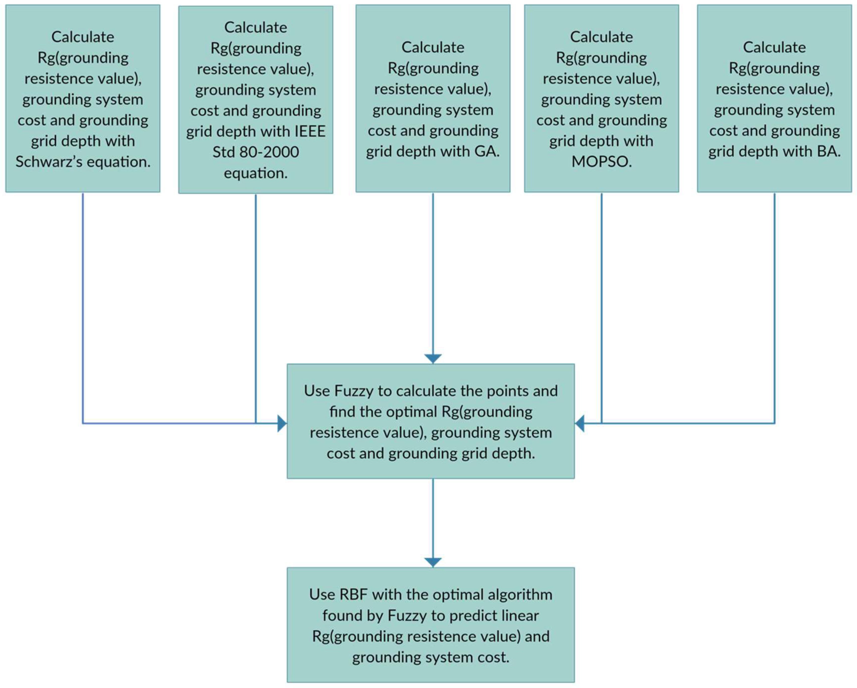
3.1. Grounding Prediction System

The grounding prediction system employed in this study can help evaluate grounding resistance and grounding system costs in any area. The system design is shown in Figure 1. Figure 1 shows designs for lightning protection systems of high-rise constructions in various regions of the world and the grounding system resistance value plus the grounding system cost planning required for transient elimination of high-energy currents, such as fault currents or lightning strikes at power company facilities. The substation design parameters are optimized by grounding systems using various algorithms, such as genetics algorithm (GA), multi-objective particle swarm optimization (MOPSO), and bee swarm algorithm (BA). The adaptive function used is dominated by the Schwarz equation to solve the grounding resistance value R_g, grounding cost, where the net grounding depth h = 0.6 m. The result is then compared to the IEEE Std. 80-2000 at h = 0.6 cm to evaluate the effectiveness. However, the grounding resistance is typically inversely proportional to the grounding grid depth and the number of grounding copper rods. In other words, in order to achieve better grounding system performance, either the grounding grid depth or the number of grounding copper rods must be increased (or both). Note that a better grounding resistance value will result in higher relative engineering costs. Based on this characteristic, the fuzzy membership function is used to establish the integral to identify the best algorithm. The fuzzy membership function identified MOPSO as the optimal algorithm from among GA and Bee. Therefore, the depth of the grounding network is optimized at 0.4–0.6 m to find the best grounding resistance value and number of grounding copper rods in a radial basis function (RBF) prediction module.

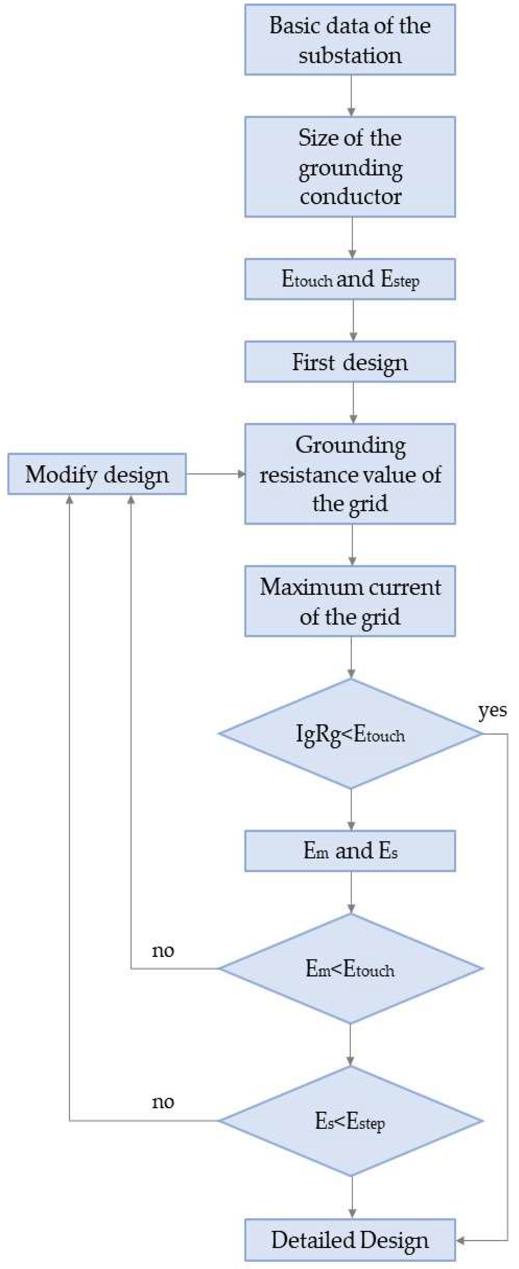
3.2. Grounding Resistance Design

The current design of the grounding system, used by Taiwan Electric Power Co., Ltd., calculates the maximum allowable touch voltage and the grounding resistance target value according to the grounding design criterion (i.e., the safe voltage that the human body can withstand). In addition, the design calculates the grounding resistance using the grounding system data in the guideline that has been stated by the Taiwan Power Company’s Electric Power Construction Unit. As stated previously, the value must be less than the target value. Calculations of the grounding resistance in the grounding design criteria are based on the planned area of the grounding grid associated with the ground network node. IEEE Std. 80-2000 is used to calculate the grounding resistance (${\mathrm{R}}_{\mathrm{g}}$ designed value) of E_m, E_s, E_touch, E_step, GPR, the total number of grounding rods, the measurement report of the depth resistivity of the base of Taipower Institute of Research, as well as the area, length, and width of the grounding grid. Simultaneously, the grounding resistance is calculated precisely using Schwarz’s equation, where the value must be less than the target value. At present, the surface resistivity coefficient is gravel 3000, and the ground network is buried at a depth of 0.6 m. The company uses Microsoft Excel 2010 to design the grounding system to perform calculations for item (2) IEEE Std. 80-2000. The ground resistance design flow is illustrated in Figure 2.

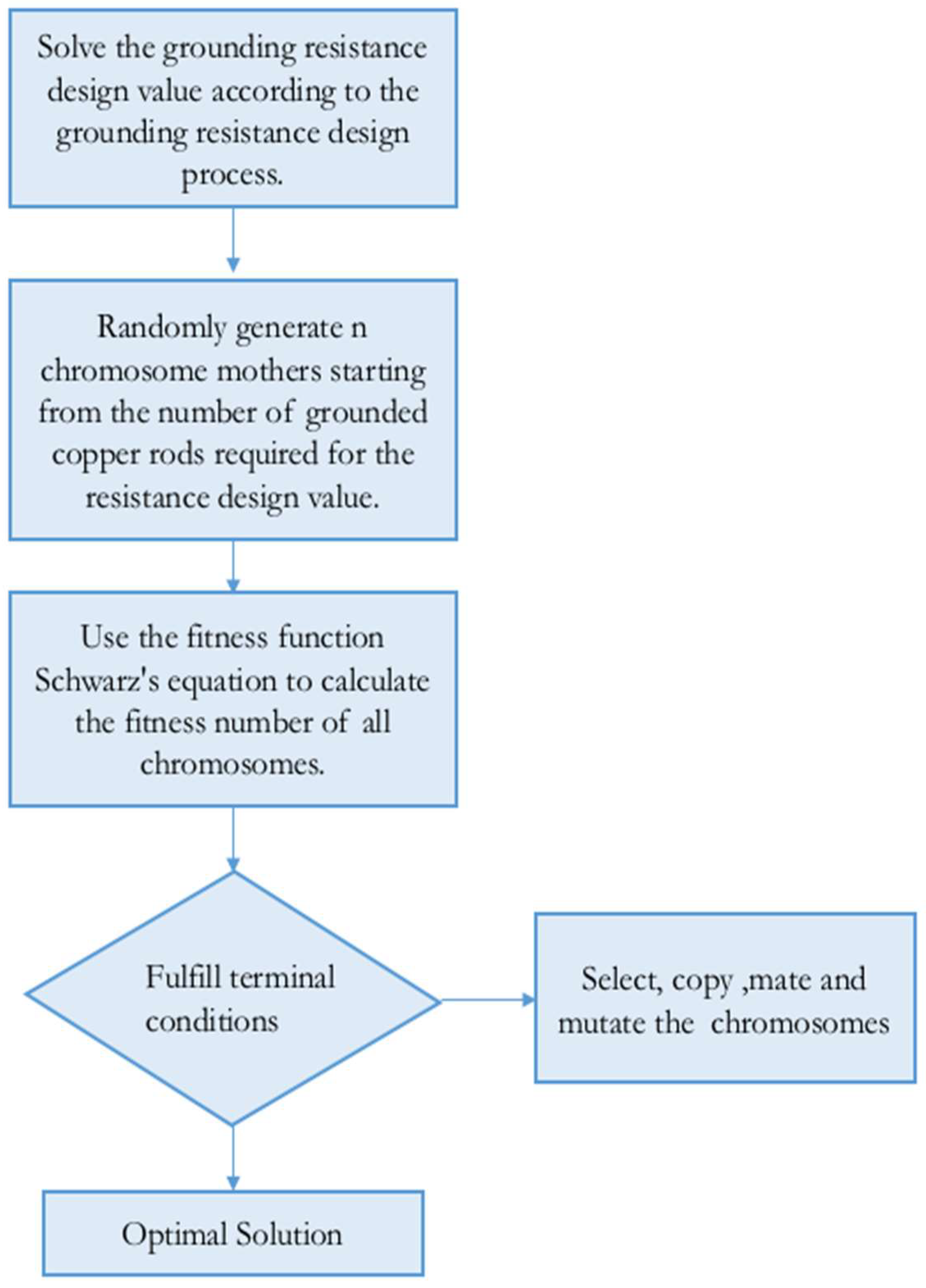
3.3. GA Optimization Flow Chart

The flow chart of the grounding system designed using GA optimization [14] is shown in Figure 3. According to the grounding resistance design process, the number of grounded copper rods required to solve the grounding resistance design value is used as the chromosome mother number. Since there are numerous grounding system data items collected by the grounding target value, it is necessary to determine the search range, by designing the number of grounded copper rods, and to use Schwarz’s equation in an adaptive function calculation.

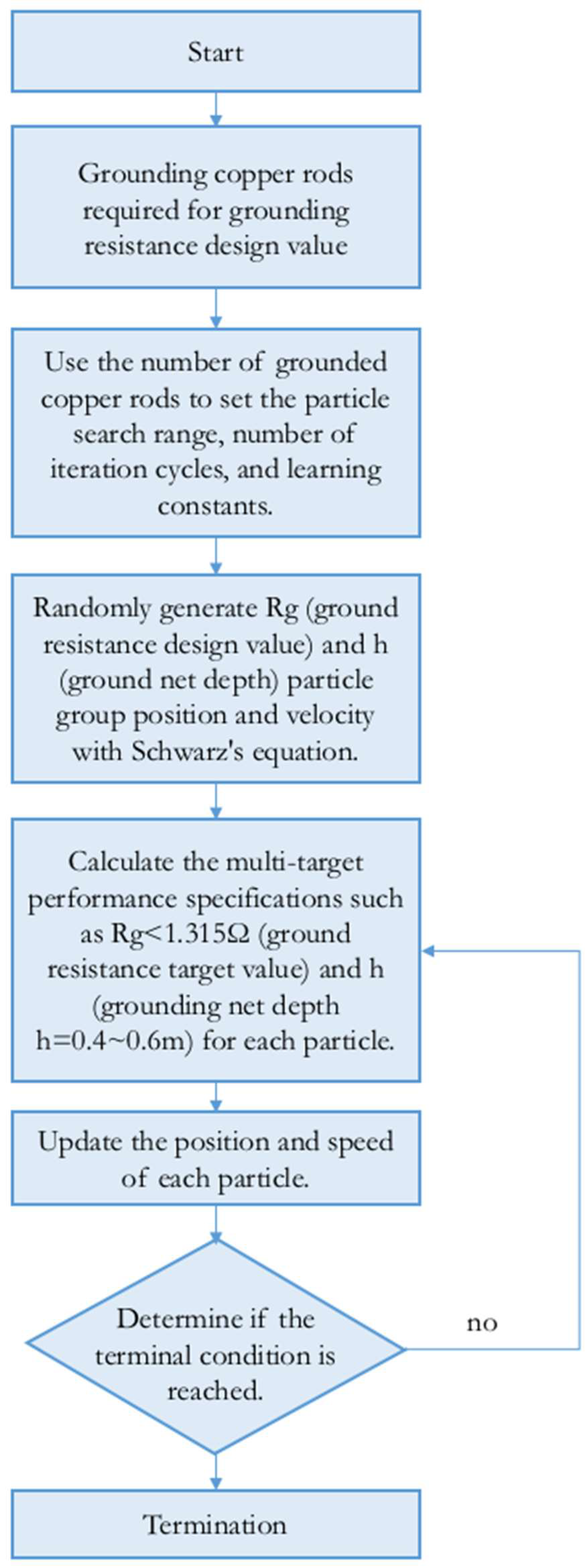
3.4. MOPSO Flow Chart

In the MOPSO flow chart [15,16,17], the number of grounding copper rods required to ground the resistance design value is calculated on the basis of the ground resistance design flow chart. There are many grounding system data items collected by the grounding target value; thus, it is necessary to determine the search range by determining an effective number of grounding copper rods for optimization, and to use Schwarz’s equation as the adaptive function, as shown in Figure 4.

3.5. Artificial Bee Swarm Algorithm Flowchart

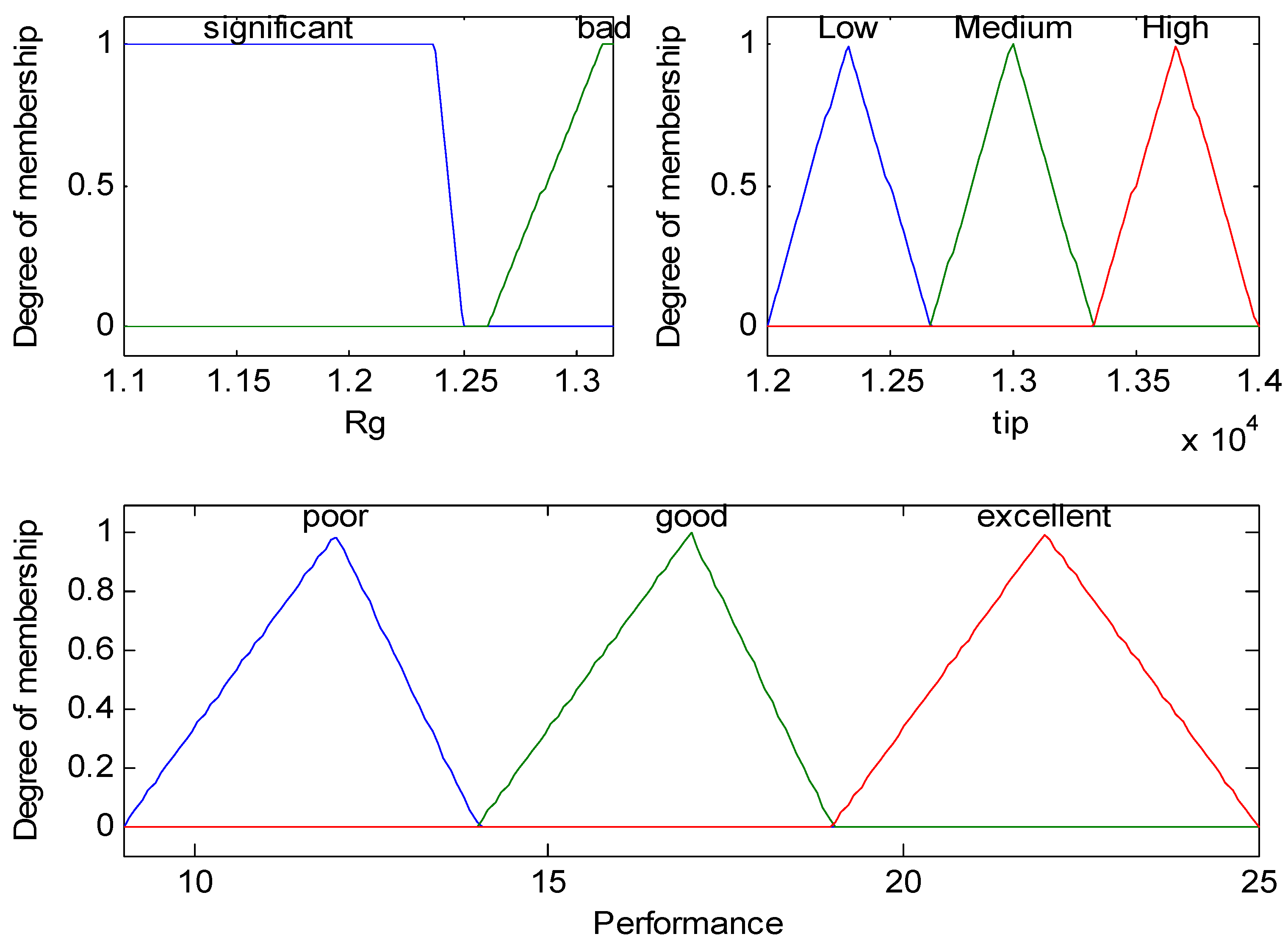
As for the grounding system that employs the artificial bee colony algorithm [18], the number of grounded copper rods is used as the initial value for the grounding resistance design. Furthermore, the search solution m is divided into a local search using the adaptation function of the Schwarz’s function as a local search. The optimal solution e is determined from an m local search; further, the optimal global solution is updated until the terminal condition is reached, as depicted in Figure 5.

3.6. Fuzzy Integral

The fuzzy rule [19] semantic notation is summarized as follows: If (x is A) and (y is B), then (z is α), and if (x is A) or (y is C), then (z is β); this expression represents the Fuzzy logic grammar. This study employs a fuzzy membership function. The two established inputs are R_g (grounding resistance) and tip (engineering cost), as depicted in Figure 6. Further, the conditions can be given as follows:

If (R_g is bad i.e., R_g (designed value) > Re (target value) = 1.315 Ω) or (tip is high), then (performance is poor).

(13)

If (R_g is significant), then (performance is good).

(14)

If (R_g is significant) and (tip is low), then (performance is excellent).

(15)

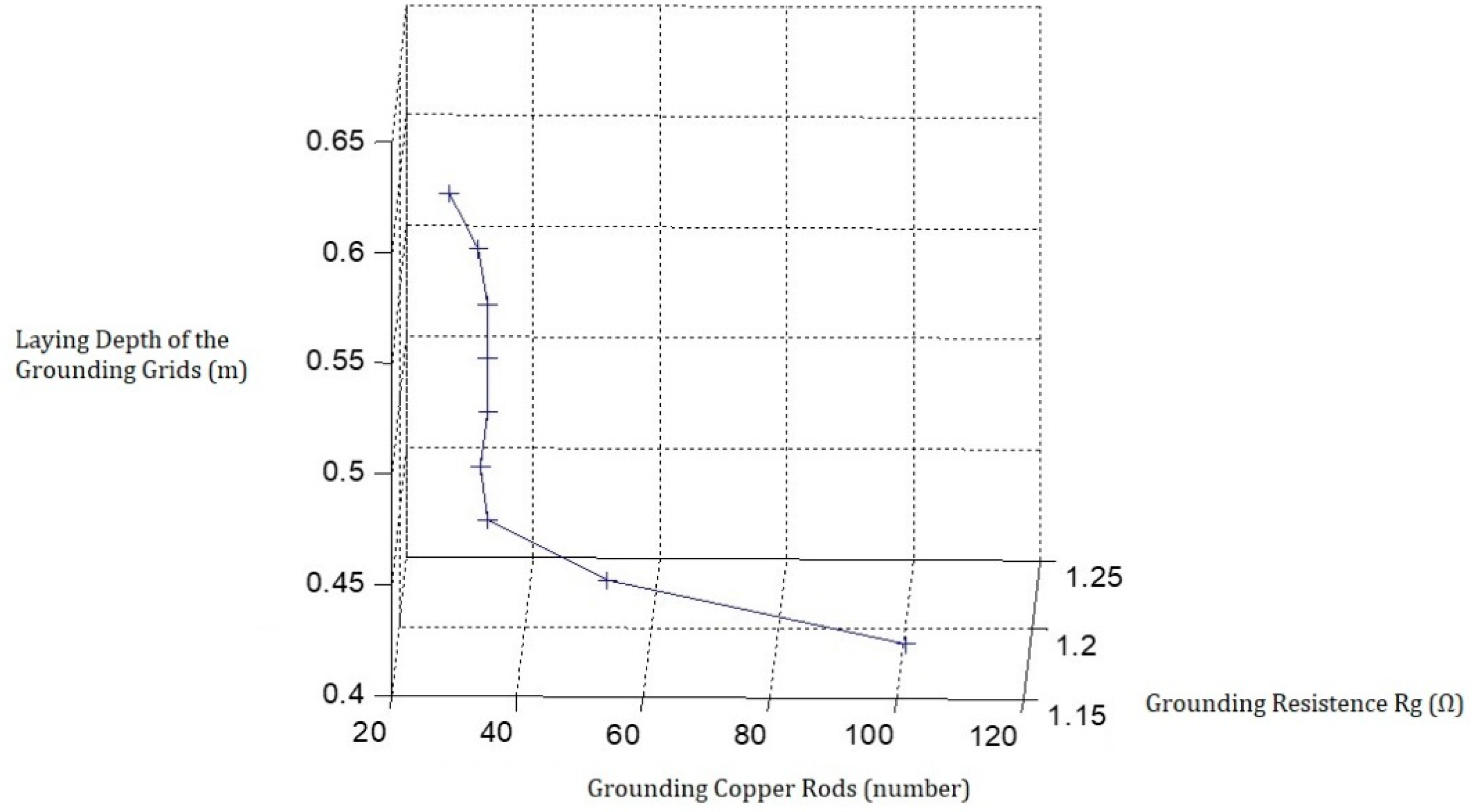
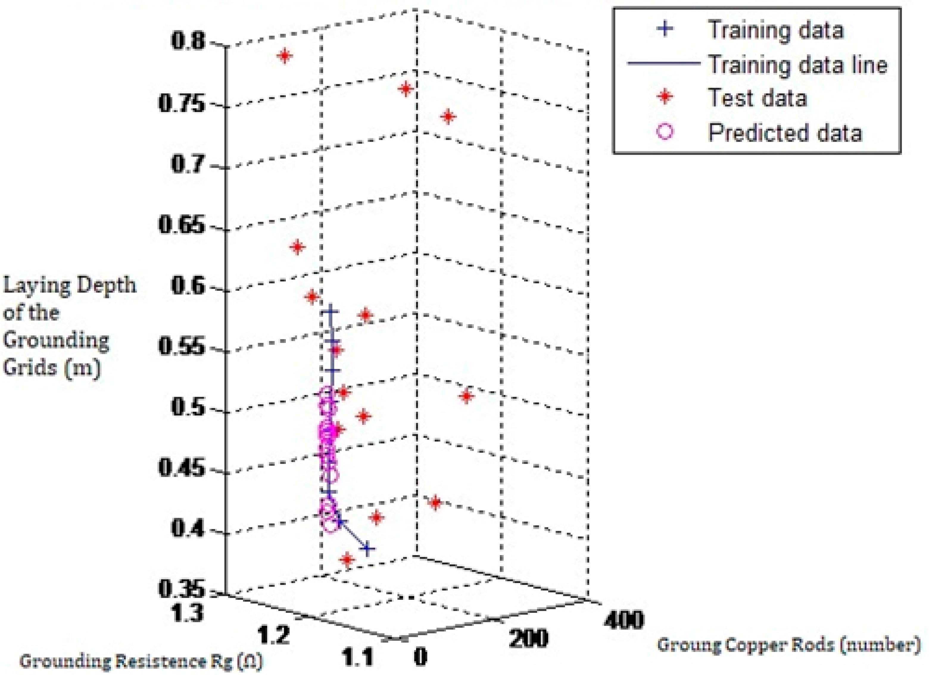
3.7. RBF Neural Network

The RBF neural network [20] is the first function to use the real multivariate interpolation method. Its main structure can be divided into three layers. The first layer is the input layer with input dimension p, and the second layer is the hidden layer, that is, a nonlinear transformation from the input layer space to the hidden layer space, which is an application of high-dimensional space. The third layer is the output layer, which is converted by the activation function of the network. The output of the third layer has linearly-segmentable features. To predict the grounding resistance value of the soil layer in any area, the number of grounding copper rod, grounding depth of the grounding grid, and other grounding parameters, the three variable values of the grounding parameter are input into nine neurons of every input variable of the hidden layer along with the three output variables. The RBF neural network of the hidden layer neurons (i.e., the basis function used by the neuron output) is dominated by a Gaussian function, and its mathematical representation is expressed as follows:

$${\mathsf{\varphi }}_{\mathrm{j}}(\mathrm{x})=\exp (\frac{{\left|\mathrm{x}-{\mathrm{m}}_{\mathrm{j}}\right|}^2}{2{{\mathsf{\sigma }}_{\mathrm{j}}}^2}).$$

(16)

4. System Simulation

Typically, the grounding resistance value is inversely proportional to the laying depth of the grounding grid and the number of grounded copper rods. In order to achieve a better grounding system performance, the laying depth of the grounding grid and the number of grounded copper rods should be either alternatively or simultaneously increased. A better grounding resistance value results in a higher relative engineering cost. The fuzzy algorithm is more suitable to comparatively evaluate the degree of goodness and weakness of the entire system with various algorithms. The grounding resistance value and grounding system engineering cost are taken as fuzzy input/disadvantage scores to identify the best algorithm relative to outputting the fuzzy integral score (

Table 1. Fuzzy integrals of grounding data for each algorithm in the fixed network laying depth.

Parameters of the Grounding-Parameter Algorithm	Grounding Copper Rod (n)	Ground Network Excavation Depth (m)	Grounding Resistance (Ω)	Project Cost	Fuzzy Integral
Schwarz’s equation	82	0.6	1.24	13,136.76 USD	15.0000
IEEE Std. 80-2000	82	0.6	1.19	13,136.76 USD	15.0000
GA	61	0.6	1.25	12,832.05 USD	15.0000
MOPSO	28	0.6	1.24	12,353.22 USD	19.9989
Bees	139	0.6	1.14	13,963.83 USD	13.2965

Grounding copper rod price: approx. 14.51 USD. Grounding network excavation cost: 7.24 USD/m (total ground line length: approximate 1650.13 m). Ground net area: 75 × 67 m; target value < 1.315 Ω.

). Among the various algorithms used, the MOPSO integral of 19.9989 was the highest input, as shown in Table 1. Therefore, MOPSO was used as the input module for subsequent prediction of the grounding system data.

MOPSO is the most suitable algorithm for the grounding system relative to predicting various grounding data. In order to quickly establish the prediction line of the grounding system, MOPSO’s adaptation function (i.e., Schwarz’s equation) is replaced by IEEE Std. 80-2000, which has a small value gap, as a prediction line adaptation function. The trend of grounding rods used and the grounding resistance value simulating grounding grid depth at 0.1–0.6 m is shown in Figure 7. Here, after MOPSO simulated-result for h = 0.35 m, R_g = 1.3482 Ω exceeded the design target value R_g = 1.315 Ω of this substation. Thus, we used h = 0.4–0.6 m as a sample for the input of the ground resistance prediction line simulation. The follow-up MOPSO simulation results are given in

Table 2. Simulation results of the adaptation function for IEEE Std. 80-2000 by MOPSO at grounding grid depths of h = 0.4–0.6 m.

Laying Depth of Grid (m)	Grounding Copper Rod (n)	Grounding Resistance Rg (Ω)
h = 0.4 m	101	1.1897
h = 0.425 m	53	1.1949
h = 0.45 m	34	1.1967
h = 0.475 m	33	1.1960
h = 0.5 m	34	1.1950
h = 0.525 m	34	1.1942
h = 0.55 m	34	1.1934
h = 0.575 m	33	1.1927
h = 0.6 m	28	1.1926

. The data in Table 2 were used to create a three-dimensional (3D) space curve, as shown in Figure 8. To construct a general model of grounding parameters, such as the grounding resistance value, grounding copper rods, and ground net depth for any region, any of the three variable values of the parameters in Table 2 is inputted into RBF neural networks. The constructed neural network can input any grounding resistance, grounding copper rod, and grounding grid depth parameter values. After the RBF neural network process, the results mostly pass through the prediction line of the IEEE Std. 80-2000 adaptation function calculated by MOPSO, as shown in Figure 9.

After the MOPSO calculation, the best result of the IEEE Std. 80-2000 adaptation function was at a grounding depth h = 0.6 m, grounding resistance 1.1926 Ω, and 28 grounded copper rods (the other related parameter data are given in Appendix A). ETAP [21] ver. 4.0.0. is a simulating software. We use the finite element method (FEM) of the ETAP toolbox to construct the grounding copper rod, grounding depth of the grounding grid, and other grounding parameters that are required to perform the simulation [22], as depicted in Figure 10. The simulation results of the best grounding parameters for the prediction line of the RBF neural network grounding system comply with ${\mathrm{E}}_{\mathrm{m}}$ = 686.3 V < ${\mathrm{E}}_{\mathrm{touch}50}$ = 775.8 V, ${\mathrm{E}}_{\mathrm{s}}$ = 593.9 V < ${\mathrm{E}}_{\mathrm{step}50}$ = 2611 V, and GPR = 4096.2 V > ${\mathrm{E}}_{\mathrm{touch}50}$ = 775.8 V, with a considerable safety margin (Figure 11). The result of ETAP simulating a 50 kg human body using ${\mathrm{I}}_{\mathrm{f}}$ was R_g = 1.19 Ω, which is similar to the set of ground resistance values obtained by the MOPSO algorithm at a grounding grid depth of 0.4–0.6 m. Figure 12, Figure 13 and Figure 14 show 3D plots of the step voltage, touch voltage, and absolute voltage for the ETAP simulations, respectively.

5. Conclusions

The contributions of this paper may be summarized as follows.

(1)

The grounding system data were optimized with numerous set solutions for GA, MOPSO, and Bees for same grounding target values.

(2)

By establishing a fuzzy integral table to count the score of the optimization algorithms, IEEE Std 80-2000, and Schwarz, we identified a suitable algorithm for optimizing the grounding system.

(3)

Using the RBF neural network as the prediction line of the grounding system is conducive to different soil layer resistivity in different regions, and it can predict the optimal grounding resistance and grounding system cost.

In future, these approaches can be optimized using optimization algorithms for uniform and non-uniform grounding grids as research directions.

References

1. IEEE. Std 80TM-2013: Revision of IEEE Std 80-2000, IEEE Guide for Safety in AC Substation Grounding; American National Standards Institute (ANSI): Washington, DC, USA, 2015. [Google Scholar]
2. Dalziel, C.F.; Mansfield, T.H. Effect of frequency on perception currents. Trans. Am. Inst. Electr. Eng. 1950, 69, 1161–1168. [Google Scholar] [CrossRef]
3. Dalziel, C.F.; Ogden, E.; Abbott, C.E. Effect of frequency on let-go currents. Trans. Am. Inst. Electr. Eng. 1943, 62, 745–750. [Google Scholar] [CrossRef]
4. Alik, B.; Teguar, M.; Mekhaldi, A. Optimization of grounding system of 60/30 kV substation of Ain el-Melh using GAO. In Proceedings of the 4th International Conference on Electrical Engineering (ICEE), Boumerdes, Algeria, 13–15 December 2015. [Google Scholar]
5. Alik, B.; Teguar, M.; Mekhaldi, A. Minimization of grounding system cost using PSO, GAO, and HPSGAO techniques, IEEE Trans. Power Deliv. 2015, 30, 2561–2569. [Google Scholar] [CrossRef]
6. IEC TS 60479-1(1994-09), Effect of Current Passing through Human Body—Part I: General Aspects. Available online: https://webstore.iec.ch/publication/16330 (accessed on 29 September 1994).
7. Dalziel, C.F. Dangerous electric currents. Trans. Am. Inst. Electr. Eng. 1946, 65, 579–585. [Google Scholar] [CrossRef]
8. Dalziel, C.F.; Massoglia, F.P. Let-go currents and voltages. AIEE Trans. Part II Appl. Ind. 1956, 75, 49–56. [Google Scholar] [CrossRef]
9. Dalziel, C.F.; Lagen, J.B.; Thurston, J.L. Electric shock. Trans. Am. Inst. Electr. Eng. 1941, 60, 1073–1079. [Google Scholar] [CrossRef]
10. Dalziel, C.F. Electric Shock Hazard. IEEE Spectr. 1972, 9, 41–50. [Google Scholar] [CrossRef]
11. Dalziel, C.F.; Lee, W.R. Reevaluation of lethal electric currents. AIEE Trans. Ind. Gen. Appl. 1968, IGA–4, 467–476. [Google Scholar]
12. El-Tous, Y.; Alkhawaldeh, S.A. An efficient method for earth resistance reduction using the Dead Sea water. Energy Power Eng. 2014, 6, 47–53. [Google Scholar] [CrossRef]
13. Schwarz, S.J. Analytical expressions for the resistance of grounding systems. Trans. Am. Inst. Electr. Eng. Part III Power Appar. Syst. 1954, 73, 1011–1016. [Google Scholar]
14. Holland, J. Adaptation in Natural and Artificial System; University of Michigan Press: Ann Arbor, MI, USA, 1975. [Google Scholar]
15. Kennedy, J.; Eberhart, R. Particle swarm optimization. In Proceedings of the Fourth IEEE International Conference on Neural Networks, Perth, Australia, 27 November–1 December 1995; pp. 1942–1948. [Google Scholar]
16. Shi, Y.; Eberhart, R.C. A modified Particle swarm optimization. In Proceedings of the IEEE International Conference on Evolutionary Computation (ICEC), Anchorage, Alaska, 4–9 May 1998; pp. 69–72. [Google Scholar]
17. Hu, X.; Shi, Y.; Eberhart, R.C. Recent advances in particle swarm. In Proceedings of the IEEE Congresson Evolutionary Computation, Portland, OR, USA, 19–23 June 2004; Volume 2, pp. 90–97. [Google Scholar]
18. Pham, D.T.; Ghanbarzadeh, A.; Koc, E.; Otri, S.; Rahim, S.; Zaidi, M. “The Bees Algorithm,” Technical Note; Manufacturing Engineering Centre, Cardiff University: Cardiff, UK, 2005. [Google Scholar]
19. Zadeh, L.A. Fuzzy sets. Inform. Control 1965, 8, 338–353. [Google Scholar] [CrossRef] [Green Version]
20. Chang, Y.W.; Hsieh, C.J.; Chang, K.W.; Ringgaard, M.; Lin, C.J. Training and testing low-degree polynomial data mappings via linear SVM. J. Mach. Learn. Res. 2010, 11, 1471–1490. [Google Scholar]
21. Tabatabaei, N.M.; Mortezaeei, S.R. Design of grounding systems in substations by ETAP intelligent software. Int. J. Tech. Phys. Probl. Eng. (IJTPE) 2010, 2, 45–49. [Google Scholar]
22. Lee, H.S.; Kim, J.H.; Dawalibi, F.P.; Ma, J. Efficient ground designs in layered soils. IEEE Trans. Power Deliv. 1998, 13, 745–751. [Google Scholar]
Figure 1. Grounding prediction system.
Energies 11 03484 g001
Figure 2. Grounding resistance design flow.
Energies 11 03484 g002
Figure 3. Flow of the grounding system with GAO.
Energies 11 03484 g003
Figure 4. Flow of the grounding system with MOPSO.
Energies 11 03484 g004
Figure 5. Flow of the grounding system with artificial bee colony algorithm optimization.
Energies 11 03484 g005
Figure 6. Membership functions of inputs Rg (ground resistance) and tip (project cost) and the output performance.
Energies 11 03484 g006
Figure 7. IEEE Std. 80-2000 adaptation function calculated by MOPSO at grounding grid depths of 0.1–0.6 m. The first objective is the number of grounding copper rods; the second objective is the trend of grounding resistance value (Ω) (red stars represent the local l best; black circles represent the global best).
Energies 11 03484 g007
Figure 8. Prediction line of the IEEE Std. 80-2000 adaptation function by MOPSO for h = 0.4–0.6 m.
Energies 11 03484 g008
Figure 9. Prediction line calculation results by an RBF neural network.
Energies 11 03484 g009
Figure 10. FEM mode grounding network completion diagram.
Energies 11 03484 g010
Figure 11. FEM simulation results with the best ground grid parameters predicted by the RBF neural network.
Energies 11 03484 g011
Figure 12. 3D plots of FEM mode step voltage.
Energies 11 03484 g012
Figure 13. 3D plots of FEM mode touch voltage.
Energies 11 03484 g013
Figure 14. 3D plots of FEM mode absolute voltage.
Energies 11 03484 g014