A Two-Step Methodology for Free Rider Mitigation with an Improved Settlement Algorithm: Regression in CBL Estimation and New Incentive Payment Rule in Residential Demand Response

Abstract

Recent demand response (DR) research efforts have focused on reducing the peak demand, and thereby electricity prices. Load reductions from DR programs can be viewed as equivalent electricity generation by conventional means. Thus, utility companies must pay incentives to customers who reduce their demand accordingly. However, many key variables intrinsic to residential customers are significantly more complicated compared to those of commercial and industrial customers. Thus, residential DR programs are economically difficult to operate, especially because excess incentive settlements can result in free riders, who get incentives without reducing their loads. Improving baseline estimation accuracy is insufficient to solve this problem. To alleviate the free rider problem, we proposed an improved two-step method—estimating the baseline load using regression and implementing a minimum-threshold payment rule. We applied the proposed method to data from residential customers participating in a peak-time rebate program in Korea. It initially suffered from numerous free riders caused by inaccurate baseline estimation. The proposed method mitigated the issue by reducing the number of free riders. The results indicate the possibility of lowering the existing incentive payment. The findings indicate that it is possible to run more stable residential DR programs by mitigating the uncertainty associated with customer electricity consumption.

1. Introduction

In demand response (DR) programs, electricity consumers play a significant role in power system operations in terms of reducing their electricity usage during system peak load in response to a time-based rate or incentive payment [1]. DR is implemented to avoid expensive electricity or peak demand prices and operated by a utility or an independent system operator (ISO). Recently, DR programs have emerged globally as an interesting approach for accommodating the high penetration of renewable energy sources. Although much effort has been made to increase renewable energy uptake to help solve environmental issues, their inherent uncertainties complicate balancing demand against supply. Therefore, there have been many attempts to utilize DR resources to ensure that they can respond faster than conventional resources, thereby facilitating stable power systems.

Of the various incentive-based DR programs, this paper focuses exclusively on peak-time rebate (PTR) programs. These programs are normally offered to residential consumers, and they provide financial incentives based on how much participants curtail their usage during specified times known as events—each event usually lasts 3 or 4 h for residential DR programs [2]. The most important aspect of DR program operation is accurate estimation of the amount of demand reduction by individual DR participants during the event period in order to pay appropriate incentives to them. The demand reduction is calculated as the difference between the customer baseline load (CBL), i.e., their estimated demand if there was no event, and the actual load during the event [3]. Thus, the CBL must be predicted precisely so that the utility can pay the correct incentives and ensure its financial/economic sustainability.

Many studies have presented statistical methods for estimating the CBL. Historical demand-averaging and day matching are conventionally used to this end by utility companies [3,4]. regression is also a typical method used for baseline estimation [5,6,7,8]. Optimized exponential smoothing was developed based on demand and weather [5,6]. Hatton [9] performed baseline estimation of residential customers using available residential load curves from a control group that did not participate in the DR program. Additionally, machine learning has also been applied to CBL estimation to mitigate the numerous uncertainties particular to residential customers. Appling machine learning in baseline estimation can be categorized into two parts: (i) Clustering customers before the estimation and (ii) using the prediction model [2,10,11,12,13]. Examples for the first category include using k-means for estimation of clustered customers based on their load patterns [9], and implementing k-means with self-organizing map techniques [10,11] in an attempt to conduct baseline estimations using customer groups. Jazaeri et al. [2] demonstrated that estimation model-based machine learning with an artificial neural network (ANN) and polynomial extrapolation outperforms historical demand-averaging, regression, ANNs, and polynomial interpolation. Problems with regard to DR program operation, such as erroneous system operation and miscalculated payment, have been solved using probabilistic estimation [13]. However, despite the need to accurately predict the CBL to ensure economically viable DR programs, the customers must be able to understand how their CBL is being calculated, which limits practical application of machine learning methods [4,14].

Baseline estimation is similar to short-term load forecasting (STLF), which is a research area being actively investigated, because both baseline estimation and STLF provide demand forecasts for less than 24 h. STLF research has been conducted with multiple methodologies; among them, support vector regression (SVR) and support vector machines (SVMs) have been employed to predict electric load [14,15,16,17]. Hybrid parameter optimization [14] and ant colony optimization [15] have been utilized in STLF to find the best parameters for SVR. SVM with simulated annealing has been presented [15], and a genetic algorithm-based SVM has been proposed [17]. Hybrid models based on SVMs, such as hybrid autoregressive integrated moving average (ARIMA) and SVM and hybrid ANN and SVM, have also been studied [18,19,20]. ANNs have been researched in the past, and they are again being actively discussed and studied as deep learning became feasible. Many papers have proposed ANN models for STLF [21,22,23,24]: e.g., a gray neural network model including wavelet decomposition [23]. Statistical time series forecasting models, such as regression, exponential smoothing, and autoregressive moving average (ARMA), have traditionally been employed, but these models analyze their components linearly. To overcome this limitation, ARMA with a non-Gaussian process has been used to predict short-term load [25], and double-seasonal exponential smoothing has been proposed and shown to have superior performance [26,27].

Unfortunately, even with such advanced estimation algorithms, accurate baseline estimation for residential customers on the distribution side is quite difficult because of the uncertainty and variability in demand due to the various factors that affect residential customers, such as home appliance usage patterns, the number of family members, life patterns, customer occupations (i.e., schedules), and income. Moreover, these factors cause residential demand to have far more variability than commercial and industrial demand [7]. Accordingly, some utility companies that use DR programs for residential customers, such as Pacific Gas & Electric (PG&E) and San Diego Gas & Electric (SDG&E) [3], have been concerned about low accuracy in CBL estimation. In particular, CBL overestimation causes inappropriate incentive payments, potentially resulting in free riders, i.e., those who receive incentive payments despite not reducing demand during an event. Existing research indicates that in order to reduce excessive incentive payments to free riders, utility companies would need to operate DR programs aimed at targeted participants who respond well to reduction notices [3]. Barring this or other solutions that address customer participation in demand reduction, the free rider problem may occur with any CBL estimation method when used alone owing to the possibility of overestimation. Thus, CBL estimation techniques are intrinsically limited in their ability to address this problem, so the inclusion of a corrective step after CBL estimation may provide the best route to addressing the free rider problem in an algorithm.

Therefore, in this study, we propose a two-step method to address the free rider problem. In the first step, the CBL is predicted using a regression-based CBL estimation method. In the second step, the incentives are settled using a new incentive payment rule, which calculates incentives depending on load reduction for a specific baseline rate in order to avoid excessive CBL prediction. The results of this study reveal an appropriate rate for residential customers. The remainder of this paper is organized as follows. In Section 2, we present existing statistical CBL methods used for simulating baseline estimations for residential customers in DR programs. In Section 3, we present the proposed 2-step model, which ensures effective incentive settlement to minimize the scale of free riders. In Section 4, we show the amount of incentives offered by different CBL methods and present incentive payment rules for a DR program operated for residential customers in Korea. Section 5 concludes the paper and outlines ideas for further research in this area.

2. Existing Baseline Estimation Methods

The successful operation of a DR program necessitates estimation of the CBL. Therefore, given that the calculation method needs to be user-friendly, utility companies typically predict the CBL using historical load-averaging methods such as “high $\mathrm{X}$ of $\mathrm{Y}$” and “last $\mathrm{Y}$ days.” To meet the needs of residential customers as well as that of the DR program, this study considered using regression to predict the CBL. Regression is substantially more robust than historical demand-averaging methods yet far more intuitive than machine learning methods.

2.1. High X of Y

High $\mathrm{X}$ of $\mathrm{Y}$ is a simple concept that is quite intuitive to customers [4]. It uses the arithmetic mean of the demands from the $\mathrm{X}$ days with highest usage of the most recent $\mathrm{Y}$ eligible days, which are defined as days preceding the event, excluding event days, holidays, and weekends. The CBL for customer $\mathrm{i}$ on event day $\mathrm{d}$ during event period $\mathrm{t}$ can be predicted as follows [15]:

$${\mathrm{CBL}}_{\mathrm{i},\mathrm{d},\mathrm{t}}=\frac{{{\displaystyle \sum }}_{\mathrm{n}\in \mathrm{high}\left(\mathrm{X},\mathrm{Y},\mathrm{d}\right)}{\mathrm{L}}_{\mathrm{i},\mathrm{n},\mathrm{t}}}{\mathrm{X}},$$

(1)

where $\mathrm{high}\left(\mathrm{X},\mathrm{Y},\mathrm{d}\right)$ refers to the set of $\mathrm{X}$ days with highest demand among the $\mathrm{Y}$ eligible days preceding the event day, $\mathrm{d}$, and ${\mathrm{L}}_{\mathrm{i},\mathrm{n},\mathrm{t}}$ is the actual load for customer $\mathrm{i}$ on eligible day $\mathrm{n}$ during event period $\mathrm{t}$. Several utility companies and ISOs utilize this method, as shown in

Table 1. Details for the high X of Y methods used by several utility companies and independent system operators (ISOs).

Utility/ISO	CBL Method
SDG&E	high 3 of 5
Ontario	high 4 of 5
PJM	high 3 of 10
NewYork ISO	high 5 of 10
PowerCents DC	high 3 of 20, high 5 of 20, high 10 of 20

[3,4].

The limitation of this method is that it cannot consider demand changes caused by temperature changes or other variable changes because it only refers to metered historical demand for its calculations. For instance, if the temperature is relatively consistent for several days but then suddenly rises or falls on the day of the event, this method cannot reflect the sudden temperature change, so it predicts the baseline as per a usual day despite the expectedly different behavior of the customers.

2.2. Last Y Days

Similar to high X of Y, last Y days uses the arithmetic mean of historical demand for the last Y eligible days for the CBL predictions [2]:

$${\mathrm{CBL}}_{\mathrm{i},\mathrm{d},\mathrm{t}}=\frac{{{\displaystyle \sum }}_{\mathrm{n}\in \mathrm{last}\left(\mathrm{Y},\mathrm{d}\right)}{\mathrm{L}}_{\mathrm{i},\mathrm{n},\mathrm{t}}}{\mathrm{Y}},$$

(2)

where $\mathrm{last}\left(\mathrm{Y},\mathrm{d}\right)$ refers to the set of $\mathrm{Y}$ eligible days preceding the event day $\mathrm{d}$. Certain utility companies and ISOs utilize this method, as shown in

Table 2. Details of the last Y days methods used by certain utility companies and ISOs.

Utility/ISO	CBL Method
Wisconsin Energy	last 3 days
NewYork ISO	last 10 days
Ontario	last 5 days
CAISO	last 10 days, last 4 days

.

2.3. Regression

Residential electricity demand is related to many variables, such as historical demand, the number of household members, the types of appliances used by the household, humidity, and cooling degree hours (CDH; i.e., the amount that the hourly maximum temperature is above a prescribed outdoor temperature—CDH is zero if the temperature is below the prescribed outdoor temperature). Cooling load makes up a large proportion of residential demand in summer—demand increases considerably when the temperature is high owing to the use of air conditioners. In this respect, CDH, a measurement designed to quantify the amount of electricity required to cool homes, can reflect the change in demand when the temperature rises in summer. Therefore, conducting baseline estimations by identifying the relationships between electricity demand and associated variables is more useful than just using historical demand data. The baseline can be estimated through linear regression, and historical data are normally chosen as the independent variables:

$${\mathrm{CBL}}_{\mathrm{i},\mathrm{d},\mathrm{t}}=\mathsf{\alpha }+{\mathsf{\beta }}^{\mathrm{T}}{\mathrm{X}}_{\mathrm{i},\mathrm{d},\mathrm{t}}+\mathsf{\epsilon },$$

(3)

where ${\mathrm{X}}_{\mathrm{i},\mathrm{d},\mathrm{t}}$ is the feature vector, $\mathsf{\alpha }$ is a constant, $\mathsf{\beta }$ is the regression coefficient vector, and ${\mathsf{\epsilon }}_{\mathrm{i},\mathrm{d},\mathrm{t}}$ is the error. The feature vector can express the historical electricity demand, weather, CDH, humidity, sunrise/sunset time, and day of the week. Once the regression formula is formulated for baseline estimation, the regression coefficients should be determined to minimize the error by using methods such as the least-squares method and maximum-likelihood estimation. Then, the baseline can be estimated for the event. In this paper, the hourly baseline profile is calculated from hourly demand data, but regression over the sum of demand during event periods has also been utilized (e.g., SDG&E [3]). Certain utility companies and ISOs utilize this method, as shown in

Table 3. Details of the regression method uses by certain utility companies and ISOs.

Utility/ISO	CBL Method
ERCOT	Regression of energy use during previous 20 like days
BG&E	Regression of energy use during event window based on weather and day of week
SDG&E	Regression of energy use during event window based on CDH, month, and day of week

.

3. Methodology for Free Rider Mitigation in Incentive Settlements of DR Programs Offered to Residential Customers

3.1. Research Framework for the Proposed Model

The framework used to settle the incentive and evaluate the performance of the proposed model is depicted in Figure 1. First, in order to estimate the baseline, load and temperature data are collected; then, these data undergo preprocessing, which comprises data selection (i.e., excluding weekends, holidays, and event days from the data), cleansing (i.e., replacing missing data and/or deleting incomplete customer data), and reduction (i.e., calculation of CDH from temperature data for a prescribed outdoor temperature of 24 °C). After data preprocessing, CBL estimation is performed through linear regression using historical demand and CDH as the independent variables. The incentive payment is estimated after the load reduction has been calculated. The proposed model for incentive settlement institutes a new payment rule that includes a threshold rate intended to deny incentives to customers whose load reduction does not exceed the threshold. The performance of the CBL estimation and incentive settlement method was assessed to understand whether the model was suitable for the operation of a DR program.

3.2. Regression

The regression was performed using historical demand from Y eligible days and (sometimes) the CDH as the independent variables to determine which regression model that performed best in this situation. Specifically, cases without the CDH with $\mathrm{Y}\in \left\{2,3,4\right\}$ and cases with the CDH with $\mathrm{Y}\in \left\{1,2\right\}$ were considered:

$${\mathrm{CBL}}_{\mathrm{i},\mathrm{d},\mathrm{t}}=\mathsf{\alpha }+{\mathsf{\beta }}_0{\mathrm{sumCDH}}_{\mathrm{i},\mathrm{d},\mathrm{t}}+{\displaystyle \sum _{\mathrm{n}=1}^{\mathrm{Y}}}{\mathsf{\beta }}_{\mathrm{n}}{\mathrm{L}}_{\mathrm{i},\mathrm{d}-\mathrm{n},\mathrm{t}}+\mathsf{\epsilon },$$

(4)

where $\mathrm{sumCDH}$ and $\mathsf{\epsilon }$ refer to the sum of the CDH during the event and the error, respectively.

3.3. Incentive Payment Rule

The current payment rule used in Korea to settle customer incentives considers the reduction estimated by high 4 of 5, and pays 1000KRW/kWh ($0.83/kWh) for the estimated load reduction. The rules do not charge customers extra when their actual load is larger than baseline. Furthermore, this existing rule can yield free riders. However, reducing incentives according to lack of load reduction is complex [3]. Therefore, we need to identify a suitable payment rule for the customer. Although many studies have focused on DR programs, very few have designed payment rules to mitigate free riders. This study presents a new payment rule to overcome these disadvantages. This scheme assumes a payment of $0.83/kWh if the estimated demand reduction is greater than a specific baseline rate. The proposed methodology is formulated as follows:

$${\widehat{\$}}_{\mathrm{i},\mathrm{d},\mathrm{t}}=\{\begin{array}{cc}\left({\mathrm{CBL}}_{\mathrm{i},\mathrm{d},\mathrm{t}}\times \left(1-\mathrm{R}\right)-{\mathrm{L}}_{\mathrm{i},\mathrm{d},\mathrm{t}}\right)\times \mathrm{P},& {\mathrm{if} \mathrm{CBL}}_{\mathrm{i},\mathrm{d},\mathrm{s}}\times \left(1-\mathrm{R}\right)>{\mathrm{L}}_{\mathrm{i},\mathrm{d},\mathrm{s}} \mathrm{and} \mathrm{R}>0,\\ 0,& \mathrm{otherwise},\end{array}$$

(5)

where $\mathrm{R}>0$ is the ratio of demand reduction needed to receive incentive payment and $\mathrm{P}$ is the unit price of the incentive. As per this rule, customers receive incentives only if they exceed the threshold for load reduction; otherwise, the incentive will be zero. In order for the utility to optimize incentive payments, a suitable rate, ${\mathrm{R}}^{\ast }$, that minimizes the relative excess payment error must be ascertained.

Methodology for Obtaining Suitable Rate (${\mathrm{R}}^{\ast }$)

Proxy event days are considered to obtain ${\mathrm{R}}^{\ast }$, and ${\mathrm{R}}^{\ast }$ is calculated by comparing the ideal payment with the estimated payment as per the proposed incentive payment rule. First, proxy days without events are selected, and we assume that the load is artificially reduced by a ratio equivalent to that observed for real event days to generate proxy event days. Thus, hypothetical reduced demand can be compared to actual load on proxy days. Load impact, which is the average ratio of demand reduction based on the baseline estimate when customers are notified of events by the utility (i.e., actual event days), is considered to estimate ideal reduced demand:

$${\mathrm{Impact}}_{\mathrm{load}}=\frac{{\displaystyle {\sum }_{\mathrm{i}=1}^{\mathrm{m}}}{{\displaystyle \sum }}_{\mathrm{d}\in \mathrm{D}}{\displaystyle {\sum }_{\mathrm{t}=\mathrm{T}}^{\mathrm{T}+\mathrm{s}}}\left({\mathrm{CBL}}_{\mathrm{i},\mathrm{d},\mathrm{t}}-{\mathrm{L}}_{\mathrm{i},\mathrm{d},\mathrm{t}}\right)}{{\displaystyle {\sum }_{\mathrm{i}=1}^{\mathrm{m}}}{{\displaystyle \sum }}_{\mathrm{d}\in \mathrm{D}}{\displaystyle {\sum }_{\mathrm{t}=\mathrm{T}}^{\mathrm{T}+\mathrm{s}}}{\mathrm{CBL}}_{\mathrm{i},\mathrm{d},\mathrm{t}}},$$

(6)

where $\mathrm{m}$, $\mathrm{D}$, $\mathrm{T}$, and $\mathrm{s}$ are the number of residential customers, the set of event days, the start time of the event, and the event duration, respectively. The hypothetical demand, assumed as original demand reduced by the impact load, is then

$${\hat{\mathrm{L}}}_{\mathrm{i},{\mathrm{d}}^{\prime },\mathrm{t}}={\mathrm{L}}_{\mathrm{i},{\mathrm{d}}^{\prime },\mathrm{t}}\times \left(1-{\mathrm{Impact}}_{\mathrm{load}}\right),$$

(7)

where ${\mathrm{d}}^{\prime }$ is a proxy day. As ideal payment is proportional to the ideal load reduction, the ideal payment can be obtained as

$${\$}_{\mathrm{i},{\mathrm{d}}^{\prime },\mathrm{t}}=\left({\mathrm{L}}_{\mathrm{i},{\mathrm{d}}^{\prime },\mathrm{t}}-{\hat{\mathrm{L}}}_{\mathrm{i},{\mathrm{d}}^{\prime },\mathrm{t}}\right)\times \mathrm{P}={\mathrm{L}}_{\mathrm{i},{\mathrm{d}}^{\prime },\mathrm{t}}\times {\mathrm{Impact}}_{\mathrm{load}}\times \mathrm{P}.$$

(8)

While estimating the payment for proxy days, ${\widehat{\$}}_{\mathrm{i},{\mathrm{d}}^{\prime },\mathrm{t}}$, using the new payment rule, Equation (5) is used but with ${\hat{\mathrm{L}}}_{\mathrm{i},{\mathrm{d}}^{\prime },\mathrm{t}}$, substituted for ${\mathrm{L}}_{\mathrm{i},{\mathrm{d}}^{\prime },\mathrm{t}}$:

$${\widehat{\$}}_{\mathrm{i},{\mathrm{d}}^{\prime },\mathrm{t}}=\{\begin{array}{cc}\left({\mathrm{CBL}}_{\mathrm{i},{\mathrm{d}}^{\prime },\mathrm{t}}\times \left(1-\mathrm{R}\right)-{\hat{\mathrm{L}}}_{\mathrm{i},{\mathrm{d}}^{\prime },\mathrm{t}}\right)\times \mathrm{P},& {\mathrm{if} \mathrm{CBL}}_{\mathrm{i},{\mathrm{d}}^{\prime },\mathrm{t}}\times \left(1-\mathrm{R}\right)>{\hat{\mathrm{L}}}_{\mathrm{i},{\mathrm{d}}^{\prime },\mathrm{t}} \mathrm{and} \mathrm{R}>0,\\ 0,& \mathrm{otherwise}.\end{array}$$

(9)

The relative excess payment error is formulated using Equations (8) and (9):

$$\mathrm{f}\left(\mathrm{R}\right)=\frac{{\displaystyle {\sum }_{\mathrm{i}=1}^{\mathrm{m}}}{{\displaystyle \sum }}_{{\mathrm{d}}^{\prime }\in {\mathrm{D}}^{\prime }}{\displaystyle {\sum }_{\mathrm{t}=\mathrm{T}}^{\mathrm{T}+\mathrm{s}}}\left({\widehat{\$}}_{\mathrm{i},\mathrm{d}\prime ,\mathrm{t}}-{\$}_{\mathrm{i},{\mathrm{d}}^{\prime },\mathrm{t}}\right)}{{{\displaystyle \sum }}_{\mathrm{i}=1}^{\mathrm{m}}{{\displaystyle \sum }}_{{\mathrm{d}}^{\prime }\in {\mathrm{D}}^{\prime }}{\displaystyle {\sum }_{\mathrm{t}=\mathrm{T}}^{\mathrm{T}+\mathrm{s}}}{\widehat{\$}}_{\mathrm{i},{\mathrm{D}}^{\prime },\mathrm{t}}},$$

(10)

where ${\mathrm{D}}^{\prime }$ is the set of proxy event days. To obtain the optimal rate ${\mathrm{R}}^{\ast }$, $\mathrm{f}\left(\mathrm{R}\right)$ should be minimized:

$${\mathrm{R}}^{\ast }=\underset{\mathrm{R}}{\mathrm{argmin}}\mathrm{f}\left(\mathrm{R}\right).$$

(11)

If ${\mathrm{R}}^{\ast }$ is estimated using the above methodology, the utility can remit the optimal payment. In other words, the utility will minimize incentives paid to free riders.

3.4. Evaluation Metrics

3.4.1. Baseline Performance Metrics

Baseline accuracy analysis was performed using the average relative error and the sum of absolute errors as metrics to ascertain bias and goodness of fit, respectively. The average relative error indicates how accurate the estimated CBL is compared with the actual load. Naturally, a value approaching zero is desirable. Furthermore, the CBL is overestimated when it takes a positive value, whereas it is underestimated when negative. The average relative error is calculated as follows [3]:

$${\mathrm{error}}_{\mathrm{L},\mathrm{relative}}=\frac{{\displaystyle \sum }\left({\mathrm{CBL}}_{\mathrm{i},\mathrm{d},\mathrm{t}}-{\mathrm{L}}_{\mathrm{i},\mathrm{d},\mathrm{t}}\right)}{{\displaystyle \sum }{\mathrm{L}}_{\mathrm{i},\mathrm{d},\mathrm{t}}}.$$

(12)

The sum of absolute errors reflects how accurately the CBL is estimated by the DR program. It denotes the degree of deviation of the error. The estimate will be accurate when the sum of absolute errors is close to zero. The absolute sum of error is expressed as [3]

$${\mathrm{error}}_{\mathrm{L},\mathrm{absolute}}={\displaystyle \sum }\left|{\mathrm{L}}_{\mathrm{i},\mathrm{d},\mathrm{t}}-{\mathrm{CBL}}_{\mathrm{i},\mathrm{d},\mathrm{t}}\right|.$$

(13)

3.4.2. Incentive Accuracy Evaluation Metrics

The total and relative excess payments are used to assess whether incentives are paid correctly. The total error is the sum of the difference between the incentives calculated according to the actual demand reduction and those calculated by applying the proposed methodology. The provided payment is most appropriate when the total error is zero. When the value is positive, the utility overpays incentives to customers, but the utility will give fewer incentives than ideal if the value is negative. Total error can be expressed as [3]

$${\mathrm{error}}_{\$,\mathrm{total}}={\displaystyle \sum }\left({\widehat{\$}}_{\mathrm{i},\mathrm{d},\mathrm{t}}-{\$}_{\mathrm{i},\mathrm{d},\mathrm{t}}\right).$$

(14)

In addition, the relative excess payment presents the percentage of the incentive payment error [3]:

$${\mathrm{error}}_{\$,\mathrm{relative}}=\frac{{\displaystyle \sum }\left({\widehat{\$}}_{\mathrm{i},\mathrm{d},\mathrm{t}}-{\$}_{\mathrm{i},\mathrm{d},\mathrm{t}}\right)}{{\displaystyle \sum }{\widehat{\$}}_{\mathrm{i},\mathrm{d},\mathrm{t}}}.$$

(15)

These evaluation criteria have positive values when the utility provides higher-than-appropriate incentives, and they become negative when the incentive is lower than the appropriate value.

4. Case Study: Incentive Scale Analysis in a Korean Residential DR Program

Although much attention has been devoted to demand-side management, DR operations in Korea have traditionally been limited to commercial and industrial customers. However, utility companies have recently opened up DR programs to residential customers as well. As a result, the Korea Electric Power Corporation (KEPCO) has been conducting a peak-time rebate (PTR) pilot program. As an alternative to time-of-use (TOU) and critical-peak-pricing (CPP), the PTR provides incentives matching the amount of electricity reduction achieved by participants after they receive the notification to reduce their demand. The DR program in Korea has adopted the high 4 of 5 method to determine CBL. Accordingly, the PTR pilot program for residential customers in Korea has also been applied in the same manner. In order to settle incentives, we analyzed residential customer demand data from the PTR pilot program and applied the proposed two-step methodology discussed in the previous section.

4.1. Input Data

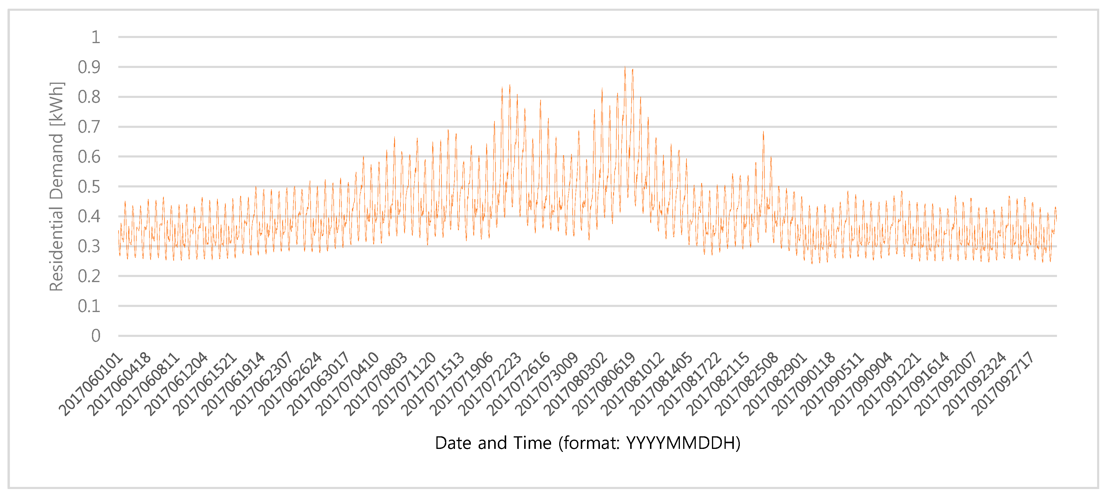
This study was conducted by using residential demand data from the case study. We obtained residential hourly demand data and temperature data in the region where the residential customers live from KEPCO and the Korea Meteorological Administration, respectively. These data included 27,660 residential customers, of which 896 participated in the PTR pilot program. The data were from June through September in 2017, during which the PTR pilot program was operated from late July to mid-September. Events occurred on 10 days in total from 13:00 to 17:00. In this paper, we considered the data for all residential customers when we evaluated CBL estimation performance; in contrast, the payment rule analysis was conducted based on the demand data from the PTR program participants to recognize the influence of incentive payments for participants in the PTR program.

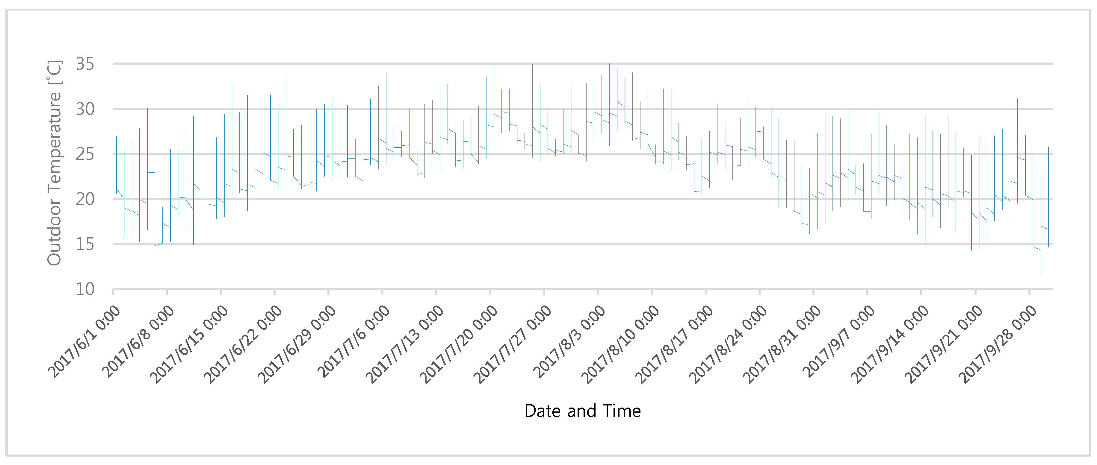
The hourly demand and temperature data are illustrated in Figure 2 and Figure 3, respectively. Figure 2 reveals that the average hourly demand for residential PTR program customers in Seoul, Korea, was highest from late July to the middle of August. However, demand was relatively low on event days, despite occurring in periods of high demand occurrence. Figure 3 confirms that the daily temperature in Seoul, Korea, has seasonal variation, with the highest temperatures occurring during daytime. The temperature was corresponding high during periods with high demand.

4.2. Proxy Day Selection

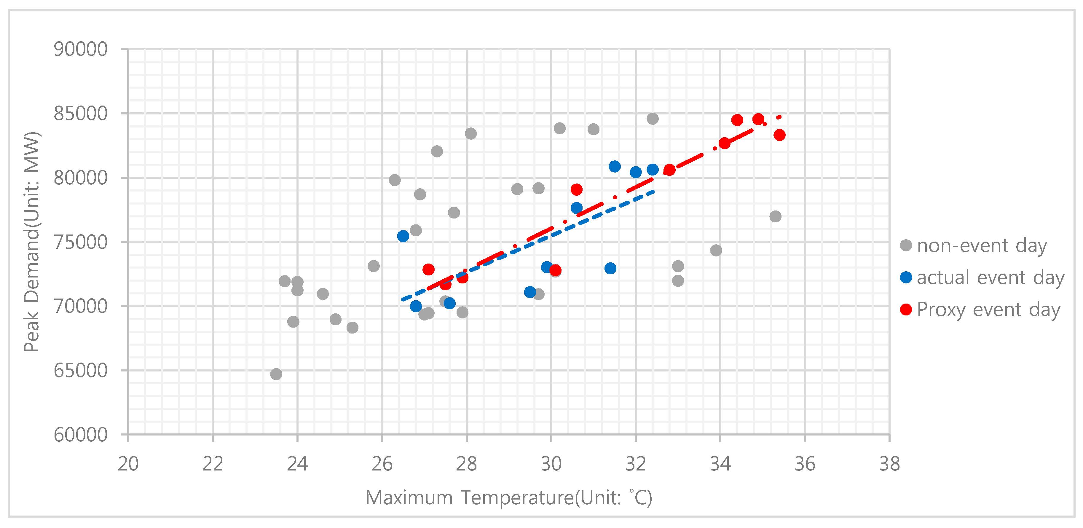
When we selected proxy event days, a similarity with event days in terms of peak demand and maximum temperature was considered. To find proxy event days, the trend line of actual event days was considered. The trend line is obtained by regression of peak demand as a dependent variable and maximum temperature as an independent variable. Then, we selected 10 proxy event days which are close to the trend line as shown in Figure 4. As shown in Figure 4, a trend line of proxy event days (blue line) is similar with the trend line of actual event days (red line). Among 10 proxy event days, five days were selected in order of similarity with the trend line of actual event days. They were used for evaluating CBL estimation accuracy and proposed payment rule. Then, suitable thresholds rate ($R^{\ast }$) was evaluated using the remaining five proxy event days. In the sensitivity analysis, the $R^{\ast }$ obtained using the remaining five proxy event days and the root rate calculated using the first five proxy event days were analyzed to investigate and compare the results.

4.3. Free Rider Problem

This study examined the accuracy of the CBL calculated for 896 residential customers in Seoul, Korea, by selecting five proxy days similar to days with real PTR events from June through September in 2017. Proxy days were selected to have peak power and average temperature similar to those of the event days. If too many proxy days were selected, the characteristics commensurate with the weather and consumption of electricity on event days, which only include hot days with high consumption during short periods in Korea, would be obscured. Similarly, SDG&E considers only the five proxy days to perform PTR baseline evaluation and evaluate incentive payment rules [3]. Therefore, the proxy days of 7 August, 14 August, 21 August, 1 September, and 5 September were selected.

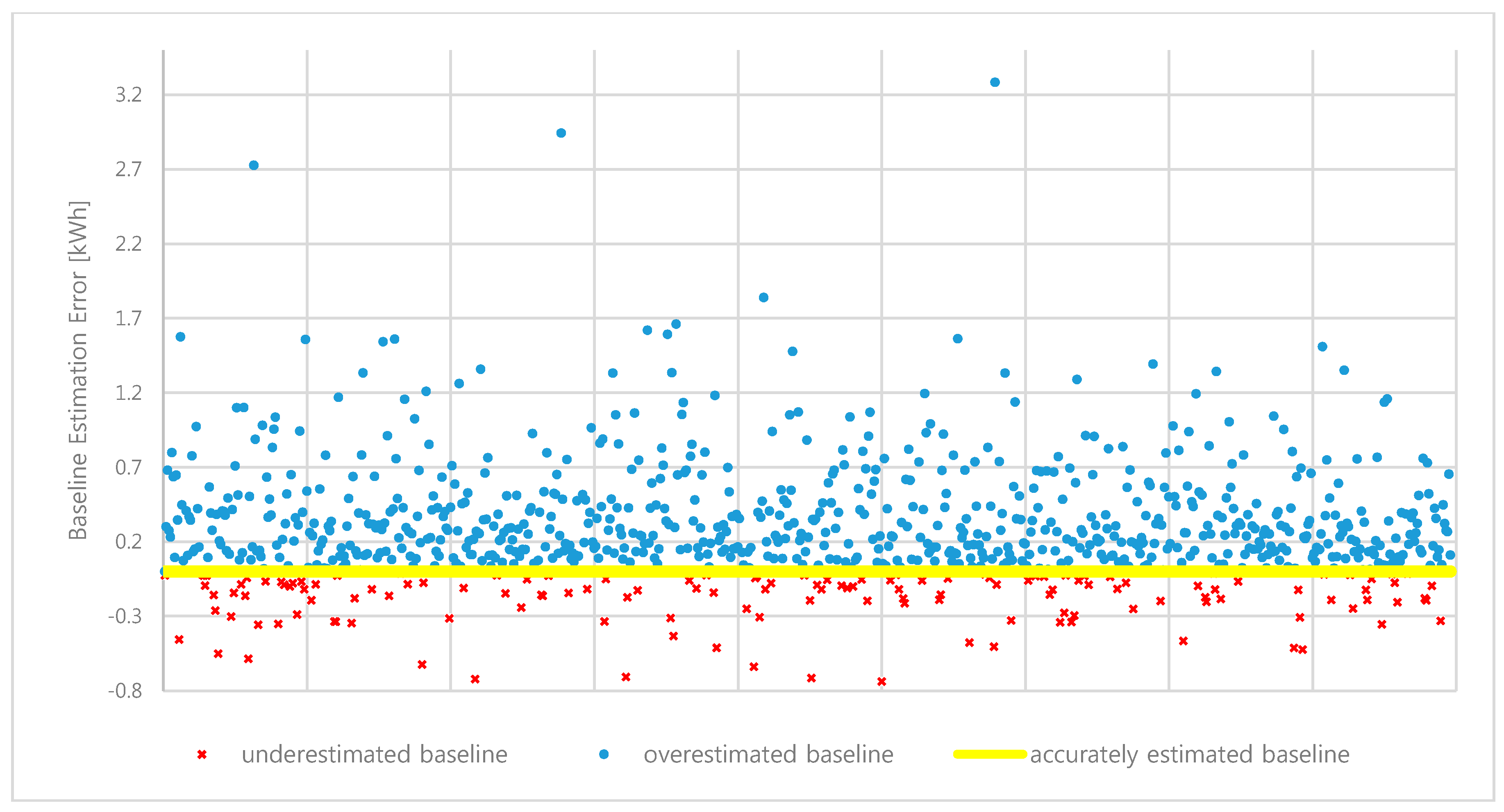
Utility companies generally use the high 4 of 5 method to determine how accurately incentives are paid to individual customers. However, the CBL is overestimated in most cases. The percentage of overestimated customers was approximately 83.04%, which indicates that 744 of 896 customers received higher than justified incentives. Customers with CBLs higher than their actual loads are free riders. This large number poses an obvious and severe financial risk. The distribution of error for these individual customers is illustrated in Figure 5. The positive and negative values signify overestimated and underestimated CBLs, respectively. Utility companies face the problem of paying additional incentives for an average of 282 kWh per event owing to overestimation by the high 4 of 5 method. As an alternative to the high 4 of 5 approach, we applied regression as the first step in the proposed methodology to reduce the number of free riders.

4.4. Results of the Regression

Baseline accuracy analysis was conducted with various baseline estimation methods, including the high 4 of 5, for the residential DR program, which serves 27,660 residential customers in Korea. As described previously, five proxy days were selected for the analysis.

4.4.1. Regression Model Selection

Before baseline accuracy analysis was conducted with the various baseline estimation methods, we established a suitable regression model for residential customers. To construct the regression models, the CDH and historical data were utilized in various combinations as independent variables in five regression models, which are described in

Table 4. Regression models.

CBL Method	Description—Derived from Equation (4)
Regression w/o CDH (4 eligible days)	${\mathrm{CBL}}_{\mathrm{i},\mathrm{d},\mathrm{t}}=\mathsf{\alpha }+{\displaystyle \sum _{\mathrm{n}=1}^4}{\mathsf{\beta }}_{\mathrm{n}}{\mathrm{L}}_{\mathrm{i},\mathrm{d}-\mathrm{n},\mathrm{t}}+\mathsf{\epsilon }$
Regression w/o CDH (3 eligible days)	${\mathrm{CBL}}_{\mathrm{i},\mathrm{d},\mathrm{t}}=\mathsf{\alpha }+{\displaystyle \sum _{\mathrm{n}=1}^3}{\mathsf{\beta }}_{\mathrm{n}}{\mathrm{L}}_{\mathrm{i},\mathrm{d}-\mathrm{n},\mathrm{t}}+\mathsf{\epsilon }$
Regression w/o CDH (2 eligible days)	${\mathrm{CBL}}_{\mathrm{i},\mathrm{d},\mathrm{t}}=\mathsf{\alpha }+{\displaystyle \sum _{\mathrm{n}=1}^2}{\mathsf{\beta }}_{\mathrm{n}}{\mathrm{L}}_{\mathrm{i},\mathrm{d}-\mathrm{n},\mathrm{t}}+\mathsf{\epsilon }$
Regression w/ CDH (2 eligible days)	${\mathrm{CBL}}_{\mathrm{i},\mathrm{d},\mathrm{t}}=\mathsf{\alpha }+{\mathsf{\beta }}_0{\mathrm{sumCDH}}_{\mathrm{i},\mathrm{d},\mathrm{t}}+{\displaystyle \sum _{\mathrm{n}=1}^2}{\mathsf{\beta }}_{\mathrm{n}}{\mathrm{L}}_{\mathrm{i},\mathrm{d}-\mathrm{n},\mathrm{t}}+\mathsf{\epsilon }$
Regression w/ CDH (1 eligible days)	${\mathrm{CBL}}_{\mathrm{i},\mathrm{d},\mathrm{t}}=\mathsf{\alpha }++{\mathsf{\beta }}_0{\mathrm{sumCDH}}_{\mathrm{i},\mathrm{d},\mathrm{t}}+{\mathsf{\beta }}_1{\mathrm{L}}_{\mathrm{i},\mathrm{d}-1,\mathrm{t}}+\mathsf{\epsilon }$

.

According to the average relative error and sum of absolute error indicators, of these regression models, regression with CDH and historical data for two eligible days (regression w/ CDH (2 eligible days)) was the best model. These results are presented in

Table 5. CBL estimation evaluation results for the considered regression models.

CBL Method	Average Relative Error [%]	Sum of Absolute Error [kWh]	Absolute Error Per Customer/Event [kWh]
Regression w/o CDH (4 eligible days)	19%	83,217	0.60
Regression w/o CDH (3 eligible days)	5%	59,780	0.43
Regression w/o CDH (2 eligible days)	5%	57,140	0.41
Regression w/ CDH (2 eligible days)	2%	61,958	0.45
Regression w/ CDH (1 eligible days)	2%	68,466	0.50

. The regression models that included CDH performed best in the aspect of bias (average relative error), but they were inferior in terms of average absolute error per customer/event (goodness of fit) to the regression models omitting CDH while using two or three days of historical data. Although inconsistent evaluation results were obtained, we concluded that regression with CDH and historical data from two eligible days was the best model because the total impact in absolute error per customer per event is small.

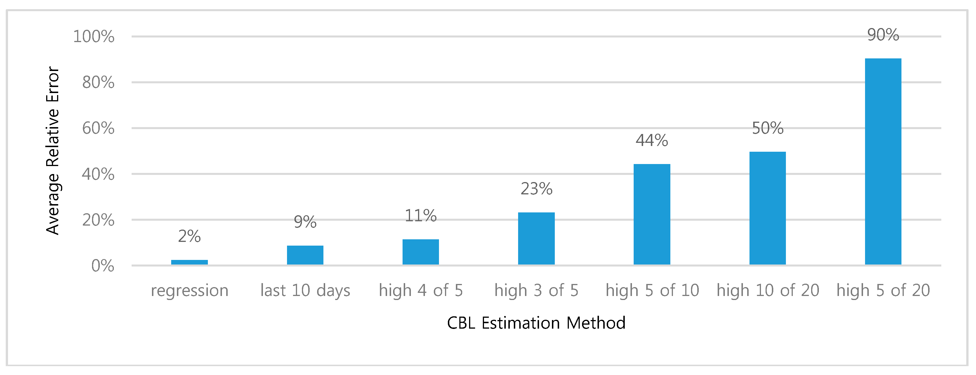
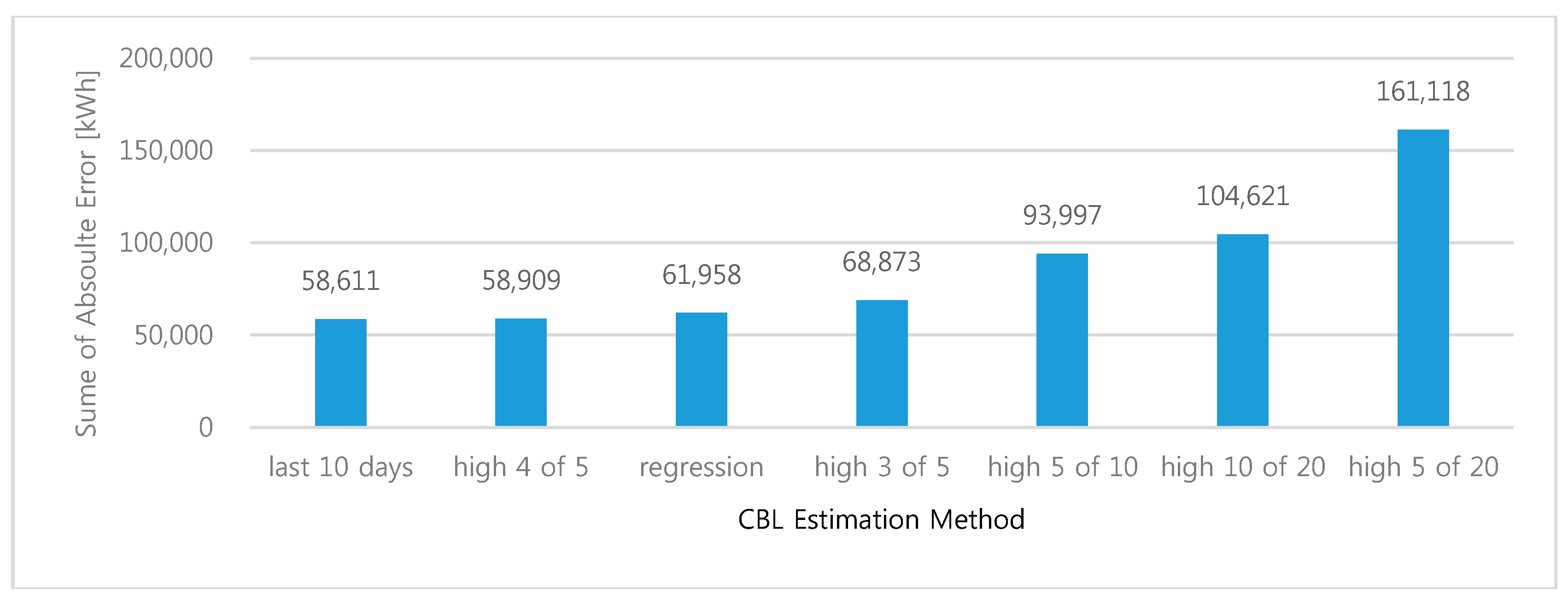
4.4.2. Performance Evaluation

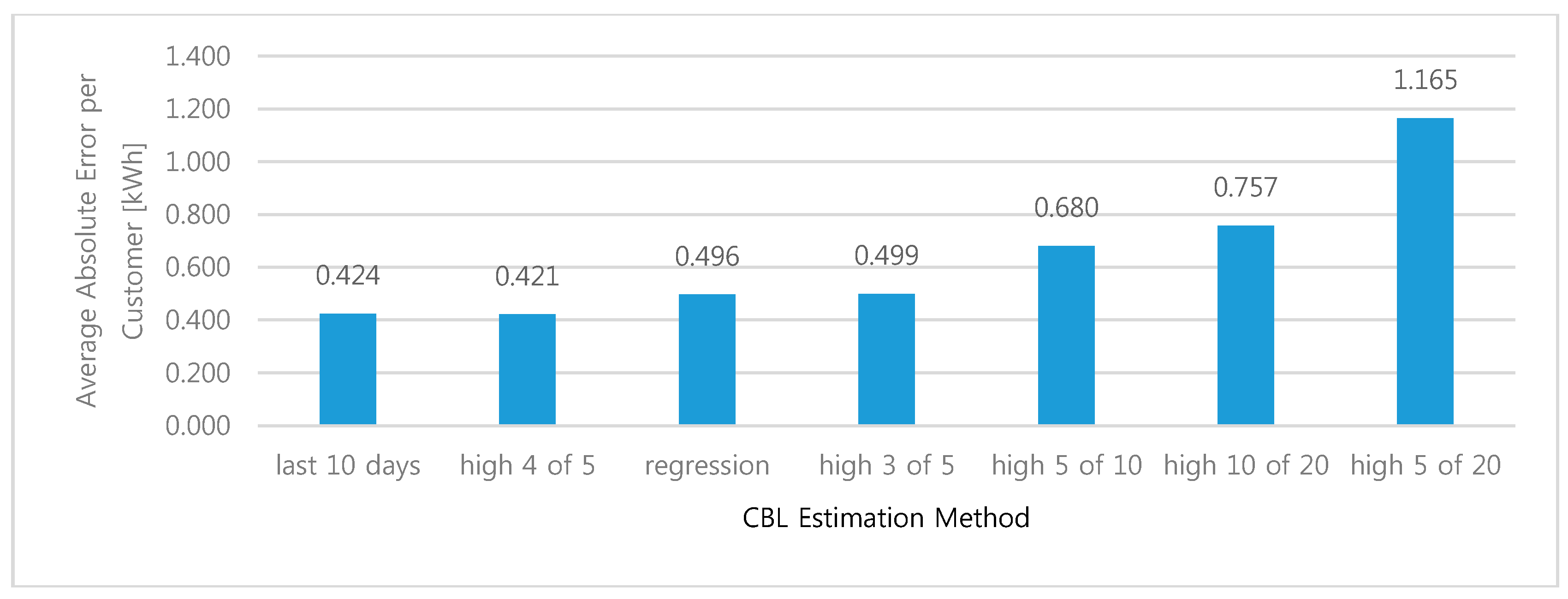
The CBL accuracy analysis was conducted for various baseline methods. The results are displayed in Figure 5, Figure 6 and Figure 7. Figure 6 shows that the regression had the smallest average relative error. Figure 7 reveals that the last 10 days method yielded the lowest sum of absolute error per event (58,611 kWh), indicating that this method was the most suitable approach with regard to accuracy. Different methods indicated the best bias and goodness of fit. The average absolute sum of error for a customer was 0.424 kWh and 0.496 kWh for the last 10 days method and the regression in Figure 8, respectively. The difference between these approaches was as low as 0.072 kWh, a very small value. Therefore, the results suggest that the regression method is the most suitable for decreasing the number of free riding residential customers.

Free riders comprised approximately 61.05% of the 547 customers as per the regression method when using the standard incentive settlement method, translating into a decrease of as many as 197 free riders. In other words, the rate of free riding declined by 21.99 percentage points for the regression method compared to the high 4 of 5 approach. The results of the baseline accuracy analysis show that while the regression method could reduce the number of free riders considerably, it could not do so entirely.

4.5. Payment Rule Analysis

The results of the CBL analysis confirmed that the regression method could improve baseline accuracy and thereby reduce payment to free riders. Nevertheless, changing the baseline method to regression still has limits; namely, the number of free riders cannot be nullified completely. Hence, we proposed a new payment rule. The proposed rule is designed to settle payment when the demand reduction is larger than a specific baseline rate. However, the suitable rate, $R^{\ast }$, for residential customers must be determined in order to use the proposed payment rule as intended. Using the methodology explained in Section 3.3, $R^{\ast }$ was determined to be 26.28%. When deriving this value, we considered other proxy days compared with the proxy days used in Section 4.3. These proxy days for obtaining $R^{\ast }$ were selected carefully because inappropriate (i.e., normal) days can result in a high rate for $R^{\ast }$. Normally, peak electricity consumption is assumed to occur on event days and proxy days; in contrast, customers use less electricity during normal days. By inappropriately including normal days as proxy days, the value of $R^{\ast }$ can increase owing to larger differences between the estimated CBL and the actual load. Excluding the 10 event days and weekends limited the selection of proxy days such that random selection of viable proxy days would have a high probability of normal day selection. Furthermore, existing research on PTR baseline evaluation conducted by SDG&E included incentive payment rule evaluation based on five proxy days [3]. For these reasons, the five proxy days selected in Section 4.3 were used to calculate $R^{\ast }$.

This paper thus compared the results obtained by applying the existing method incentive payment rule to those obtained using the proposed rule. The residential load data of the PTR pilot program implemented in Korea during the summer of 2017 were used for this analysis. In order to assess the effect of the proposed incentive payment rule, the incentive accuracy analysis for the residential DR program was conducted using the proxy days selected in Section 4.3. According to the operational results provided by the DR pilot program, the average load impact was 13.86% for the events. In other words, customers normally reduced their demand by approximately 13.86% during the events in 2017. Therefore, according to Equation (8), the ideal incentive was found to be 196,246KRW ($163.51), which can be considered an affordable incentive because the extent of load reduction should equal the load impact.

Incentive Settlement Evaluation

Using the incentive evaluation metrics described in Section 3.4.2, this study analyzed the outcomes of high 4 of 5, regression alone, and regression combined with the new payment rule. The results appear in

Table 6. Load reduction effect for various CBL estimation and payment methods.

Metric	Ideal Result	high 4 of 5	Regression	Regression and New Payment Rule
Load reduction (kWh)	197	529	391	144
Total payment ($)	163.51	439.07	324.53	119.52

and

Table 7. Payment accuracy and scale of free riders for various CBL estimation and payment methods.

Metric	high 4 of 5	Regression	Regression and New Payment Rule
Free riders (number)	744	547	81
Free rider (%)	83.04	61.05	9.04
Total error ($)	275.75	161.08	−44.05
Relative excess payment (%)	62.87	49.72	−37.07

. According to Table 6, assuming that reduction is equal to load impact, the ideal total electricity reduction, by participating customers amounted to 197 kWh; thus, the amount of actual incentives provided to these customers by the utility was $163.51. The high 4 of 5 method estimated a reduction approximately 332 kWh higher than the actual value. Therefore, the utility would have to pay its customers $275.56 more (on average) to operate the residential DR program. Similar to the previous result, the regression method was more reasonable compared with the existing method, but it still overestimated load reduction. However, the new payment rule, which pays incentives for the extent of load reduction over the threshold, yielded the most accurate load reduction after estimating the baseline by the regression method. While it offered less incentive settlement to customers, it was considerably efficient. The new payout rule reduced load impact by approximately 53 kWh compared to the actual scenario, and the incentive payment was $43.99 less than the ideal payment to the 896 customers. Additionally, the free rider problem was considerably alleviated by using the new payout method, as shown by the results in Table 7. Notably, 663 free-riding customers with overestimated CBLs were eliminated, so the free rider rate decreased to 9.04%. The distributions of customer load reduction for each method are shown in Figure 9, where the positive values represent free riders. Both the quantity and scale of free riders decreased considerably with the new payment rule compared to the traditional incentive settlement rule.

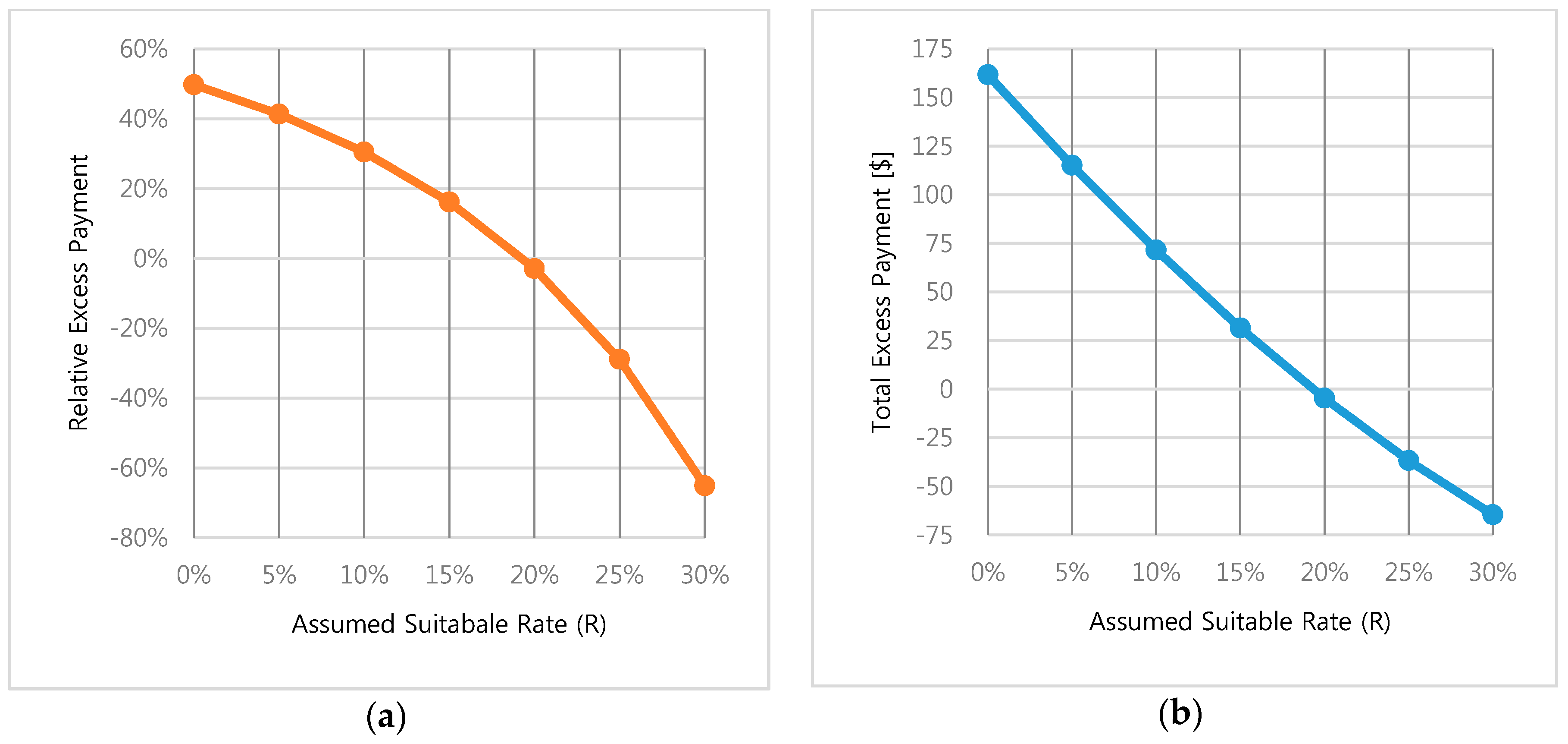
Although the proposed methodology curtailed the number of free riders, many negative values were also observed in the incentive evaluation, which means that the introduced rate may be too high. Therefore, we analyzed the payment error for a different set of proxy days according to the threshold rate. The change was confirmed by increasing the rate from 0% to 30% in increments of 5%. The results showing the relative and total excess payment values are displayed in Figure 10a,b, respectively. The relative incentive payment error gradually decreased with increasing threshold rate and fell to 0% when the threshold rate reached 19.32%. This value differs from the optimal rate because different proxy days were used to obtain the optimal rates. The results of the incentive evaluation showed a negative value when 26.28% was used as the threshold rate for the alternate proxy days.

There is a 9.96 percentage point difference between $R^{\ast }$ (26.28%) and the root rate (19.32%; i.e., the rate at which 0% relative error occurs) for the alternate proxy days. This gap could be regarded as a big difference. However, each case indicates that there is an average of 0.43 kWh or 0.32 kWh for which incentives are settled, leaving only 0.11 kWh between them. This suggests that $R^{\ast }$ is somewhat sensitive to the proxy days being selected, but for the scope of the problem, this is acceptable.

5. Conclusions

We established an incentive settlement methodology for a Korean residential DR program as a solution to the free rider problem. The proposed method outperformed other methods, especially when considering the payment rule improvement. The proposed method consists of two steps, namely, predicting the CBL using regression and implementing a minimum threshold of load for customers to receive incentive settlement. The results of the various analyses led us to the following conclusions. The proposed methodology can reliably reduce the uncertainty about free riders if it is used to predict the CBL. Using residential customer load data for Korea, we also showed that it could curtail the number of free riders. The utility can thus offer fewer (and more economically sustainable) incentives to customers. In addition, it is possible to apply this method to other DR programs with different load characteristics, as the optimal rate calculation is independent of the CBL estimation method; thus, the level of free riders can be successfully reduced. Specifically, free riders comprised approximately 61.05% of the 896 customers as per the regression method, translating into a decrease of as many as 197 free riders. With regard to incentive settlement evaluation, compared to the ideal scenario, the settled payment was $119.52 when using the regression and new payment rule, which was $43.99 lower than the ideal payment to the 896 customers in the DR program.

Although the threshold rate applied in the payment rule differs depending on which proxy days are selected, the relative difference has an acceptably minor effect on the incentive payment. If the proposed incentive payment rule were applied in a DR program, free-riding customers and those that scarcely reduce their demand would leave in this program. Beneficially, customers who significantly reduce their consumption would remain and the DR program, making operation more efficient than before. However, further research about the effect of customers leaving in accordance with threshold rate ($R^{\ast }$) in DR program would then be necessary. Overall, this methodology model is effective for mitigating the free rider problem, and it can be easily applied by simply modifying the threshold rate ($R^{\ast }$) when operating any DR program.

References

1. U.S. Department of Energy (DOE). Benefits of Demand Response in Electricity Markets and Recommendations for Achieving Them: A Report to the United States Congress Pursuant to Section 1252 of the Energy Policy Act of 2005; U.S. DOE: Washington, DC, USA, 2006. [Google Scholar]
2. Jazaeri, J.; Alpcan, T.; Gordon, R.; Brandao, M.; Hoban, T.; Seeling, C. Baseline methodologies for small-scale residential demand response. In Proceedings of the 2016 IEEE Innovative Smart Grid Technologies-Asia (ISGT-Asia), Melbourne, VIC, Australia, 28 November–1 December 2016; pp. 747–752. [Google Scholar] [CrossRef]
3. George, S.; Bode, J.; Berghman, D. 2012 San Diego Gas & Electric Peak Time Rebate Baseline Evaluation. California Measurement Advisory Council. 2012. Available online: http://www.calmac.org/publications/SDGE_PTR_Baseline_Evaluation_Report_-_Final.pdf (accessed on 13 September 2018).
4. KEMA, Inc. PJM Empirical Analysis of Demand Response Baseline Methods; KEMA, Inc.: Burlington, MA, USA, 2011. [Google Scholar]
5. Raman, G.; Kong, Y.; Peng, J.C.-H.; Ye, Z. Demand baseline estimation using similarity-based technique for tropical and wet climates. IET Gener. Transm. Distrib. 2018, 12, 3296–3304. [Google Scholar] [CrossRef]
6. Wi, Y.-M.; Kim, J.-H.; Joo, S.-K.; Park, J.-B.; Oh, J.-C. Customer baseline load (CBL) calculation using exponential smoothing model with weather adjustment. In Proceedings of the 2009 Transmission & Distribution Conference & Exposition: Asia and Pacific, Seoul, Korea, 26–30 October 2009; IEEE: Piscataway, NJ, USA, 2009; pp. 114–117. [Google Scholar] [CrossRef]
7. Mohajeryami, S.; Doostan, M.; Schwarz, P. The impact of customer baseline load (CBL) calculation methods on peak time rebate program offered to residential customers. Electr. Power Syst. Res. 2016, 137, 59–65. [Google Scholar] [CrossRef]
8. Mohajeryami, S.; Doostan, M.; Asadinejad, A.; Schwarz, P. Error analysis of customer baseline load (CBL) calculation methods for residential customers. IEEE Trans. Ind. Appl. 2016, 53, 5–14. [Google Scholar] [CrossRef]
9. Hatton, L.; Charpentier, P.; Matzner-Løber, E. Statistical estimation of the residential baseline. IEEE Trans. Power Syst. 2015, 31, 1752–1759. [Google Scholar] [CrossRef]
10. Zhang, Y.; Chen, W.; Xu, R.; Black, J. A cluster-based method for calculating baselines for residential loads. IEEE Trans. Smart Grid 2015, 7, 2368–2377. [Google Scholar] [CrossRef]
11. Park, S.; Ryu, S.; Choi, Y.; Kim, H. A framework for baseline load estimation in demand response: Data mining approach. In Proceedings of the 2014 IEEE International Conference on Smart Grid Communications (SmartGridComm), Venice, Italy, 3–6 November 2014; IEEE: Piscataway, NJ, USA, 2014; pp. 638–643. [Google Scholar] [CrossRef]
12. Park, S.; Ryu, S.; Choi, Y.; Kim, J.; Kim, H. Data-driven baseline estimation of residential buildings for demand response. Energies 2015, 8, 10239–10259. [Google Scholar] [CrossRef]
13. Weng, Y.; Rajagopal, R. Probabilistic baseline estimation via Gaussian process. In Proceedings of the 2015 IEEE Power & Energy Society General Meeting, Denver, CO, USA, 26–30 July 2015; IEEE: Piscataway, NJ, USA, 2015; pp. 606–610. [Google Scholar] [CrossRef]
14. Jiang, H.; Zhang, Y.; Muljadi, E.; Zhang, J.J.; Gao, D.W. A short-term and high-resolution distribution system load forecasting approach using support vector regression with hybrid parameters optimization. IEEE Trans. Smart Grid 2016, 9, 3341–3350. [Google Scholar] [CrossRef]
15. Niu, D.; Wang, Y.; Wu, D.D. Power load forecasting using support vector machine and ant colony optimization. Expert Syst. Appl. 2010, 37, 2531–2539. [Google Scholar] [CrossRef]
16. Pai, P.-F.; Hong, W.-C. Support vector machines with simulated annealing algorithms in electricity load forecasting. Energy Convers. Manag. 2005, 46, 2669–2688. [Google Scholar] [CrossRef]
17. Pai, P.-F.; Hong, W.-C. Forecasting regional electricity load based on recurrent support vector machines with genetic algorithms. Electr. Power Syst. Res. 2005, 74, 417–425. [Google Scholar] [CrossRef]
18. Nie, H.; Liu, G.; Liu, X.; Wang, Y. Hybrid of ARIMA and SVMs for short-term load forecasting. Energy Procedia 2012, 16, 1455–1460. [Google Scholar] [CrossRef]
19. Karthika, S.; Margaret, V.; Balaraman, K. Hybrid short term load forecasting using ARIMA-SVM. In Proceedings of the 2017 Innovations in Power and Advanced Computing Technologies (i-PACT), Vellore, India, 21–22 April 2017; IEEE: Piscataway, NJ, USA, 2017; pp. 1079–1085. [Google Scholar] [CrossRef]
20. Ray, P.; Sen, S.; Barisal, A.K. Hybrid methodology for short-term load forecasting. In Proceedings of the 2014 IEEE International Conference on Power Electronics, Drives and Energy Systems (PEDES), Mumbai, India, 16–19 December 2014; IEEE: Piscataway, NJ, USA, 2015; pp. 78–83. [Google Scholar] [CrossRef]
21. Hippert, H.S.; Pedreira, C.E.; Souza, R.C. Neural networks for short-term load forecasting: A review and evaluation. IEEE Trans. Power Syst. 2001, 16, 44–55. [Google Scholar] [CrossRef]
22. Khotanzad, A.; Hwang, R.-C.; Abaye, A.; Maratukulam, D. An adaptive modular artificial neural network hourly load forecaster and its implementation at electric utilities. IEEE Trans. Power Syst. 1995, 10, 1716–1722. [Google Scholar] [CrossRef]
23. Li, B.; Zhang, J.; He, Y.; Wang, Y. Short-term load-forecasting method based on wavelet decomposition with second-order gray neural network model combined with ADF test. IEEE Access 2017, 5, 16324–16331. [Google Scholar] [CrossRef]
24. Ding, N.; Benoit, C.; Foggia, G.; Bésanger, Y.; Wurtz, F. Neural network-based model design for short-term load forecast in distribution systems. IEEE Trans. Power Syst. 2015, 31, 72–81. [Google Scholar] [CrossRef]
25. Huang, S.-J.; Shih, K.-R. Short-term load forecasting via ARMA model identification including non-Gaussian process considerations. IEEE Trans. Power Syst. 2003, 18, 673–679. [Google Scholar] [CrossRef]
26. Taylor, J. Short-term electricity demand forecasting using double seasonal exponential smoothing. J. Oper. Res. Soc. 2003, 54, 799–805. [Google Scholar] [CrossRef] [Green Version]
27. Taylor, J.W.; McSharry, P.E. Short-term load forecasting methods: An evaluation based on European data. IEEE Trans. Power Syst. 2007, 22, 2213–2219. [Google Scholar] [CrossRef]
Figure 1. Flowchart of the proposed customer baseline load (CBL) estimation and incentive settlement method and corresponding evaluation processes.
Energies 11 03417 g001
Figure 2. Average hourly demand for residential peak-time rebate (PTR) program customers in Seoul, Korea, from June through September.
Energies 11 03417 g002
Figure 3. Hourly temperature data for Seoul, Korea, from June through September.
Energies 11 03417 g003
Figure 4. Actual event days compared to proxy event days 4.2. Free rider problem.
Energies 11 03417 g004
Figure 5. Baseline distributions when applying the high 4 of 5 method.
Energies 11 03417 g005
Figure 6. Average relative error for various CBL estimation methods.
Energies 11 03417 g006
Figure 7. Sum of absolute errors for different CBL methods.
Energies 11 03417 g007
Figure 8. Average sum of absolute error for an individual customer for different CBL methods.
Energies 11 03417 g008
Figure 9. Free rider distributions for (a) high 4 of 5, (b) regression, and (c) proposed two-step methodology using both regression and the new payment rule.
Energies 11 03417 g009
Figure 10. Variation in payment accuracy evaluation using the threshold rate, in terms of (a) relative excess payment, and (b) total excess payment.
Energies 11 03417 g010