Article

Load Rejection Transient Process Simulation of a Kaplan Turbine Model by Co-Adjusting Guide Vanes and Runner Blades

1
College of Water Conservancy and Hydropower Engineering, Hohai University, Nanjing 210098, China
2
College of Energy and Electrical Engineering, Hohai University, Nanjing 210098, China
3
Shanghai Investigation, Design & Research Institute Corporation Limited, Shanghai 200434, China
*
Author to whom correspondence should be addressed.
Energies 2018, 11(12), 3354; https://doi.org/10.3390/en11123354
Submission received: 25 September 2018 / Revised: 10 November 2018 / Accepted: 23 November 2018 / Published: 30 November 2018
(This article belongs to the Section A: Sustainable Energy)

Abstract

:
To obtain the flow mechanism of the transient characteristics of a Kaplan turbine, a three-dimensional (3-D) unsteady, incompressible flow simulation during load rejection was conducted using a computational fluid dynamics (CFD) method in this paper. The dynamic mesh and re-meshing methods were performed to simulate the closing process of the guide vanes and runner blades. The evolution of inner flow patterns and varying regularities of some parameters, such as the runner rotation speed, unit flow rate, unit torque, axial force, and static pressure of the monitored points were revealed, and the results were consistent with the experimental data. During the load rejection process, the guide vane closing behavior played a decisive role in changing the external characteristics and inner flow configurations. In this paper, the runner blades underwent a linear needle closure law and guide vanes operated according to a stage-closing law of “first fast, then slow,” where the inflection point was t = 2.3 s. At the segment point of the guide vane closing curve, a water hammer occurs between guide vanes and a large quantity of vortices emerged in the runner and the draft tube. The pressure at the measurement points changes dramatically and the axial thrust rises sharply, marking a unique time in the transient process. Thus, the quality of a transient process could be effectively improved by properly setting the location of segmented point. This study conducted a dynamic simulation of co-adjustment of the guide vanes and the blades, and the results could be used in fault diagnosis of transient operations at hydropower plants.

1. Introduction

With the dramatically worsened conflicts between energy supply and environmental protection around the world, due to the small investment, short construction period, and less negative impact on the environment, low-head hydraulic turbines have become the top priority in the development and utilization of renewable energy [1,2]. At present, Kaplan turbines are more widely used for their dual regulating function, which allows them to operate in a wide range of hydraulic conditions. Compared with higher-head turbines, Kaplan turbines can save more cost and time in the construction of power plants with lower excavation depth and less excavation of earth and rock [3,4,5].
In the daily operations of conventional hydropower stations, the frequent changes in working conditions inevitably incur transient processes of the turbine [6,7,8,9]. Load rejection is a common transient process with large fluctuations of dynamic parameters such as rotational speed, mass flow rate, torque, axial thrust, and static pressure. During the load rejection transient, the rotational speed and system water pressure rise to the effect that the flow pattern in the flow channel becomes more complex, which makes the variation regularity of external characteristics change dramatically and induce additional inertial force. The dynamic load caused by the mass imbalance in the rotor and the hydraulic instability in the flow passage components can be greatly increased by these changes, which can result in strong hydraulic pulsation and vibration and thus pose great threat to the safe operation of the entire power station [10]. Therefore, it is of great importance to ensure the operational safety of power stations with proper control schemes for regulating the turbine components. The governing components of a Kaplan turbine, namely, the guide vanes and impeller, which have unique load rejection transition processes, are particularly important to study [11,12].
Many practical transient process problems have been solved through experimental investigations [13,14,15,16,17]. Actually, many prototype tests in transient processes cannot be realized, owing to disadvantages such as large investment and some conditions being extremely dangerous, whereas numerical simulation methods are free from these problems. There are two kinds of numerical solutions for traditional transient processes. One is the numerical method of external character (NMEC) analysis, which employs the entire unit characteristics curve as the boundary condition [18]. The other is the numerical method of internal character (NMIC), which is realized by simultaneously solving the expressions of dynamic parameters with the basic equations of the pipe flow [19]. However, although these approaches can effectively predict the transient characteristics of an entire hydraulic system, especially one with a long penstock or tail water system, they are quite limited in predicting water hammer characteristics and dynamic instability of a hydro turbine unit.
In recent years, with the rapid development of large computational capacities and computational fluid dynamics (CFD), in order to directly reflect the internal flow regime of the unit, the 3-D turbulent numerical simulation method [20,21,22,23] has been introduced to study transition processes, and the research object is usually the unit section. Liu et al. [24] performed a 3-D CFD runaway transient simulation of a propeller turbine model, and some dynamic parameters and flow patterns were obtained and analyzed. Liu et al. [25,26] simulated the transient power interruption process and load rejection process of a prototype pump-turbine at pump mode by means of a 3-D flow simulation. Avdyushenko et al. [27] presented a method that was based on a joint solution to the Reynolds-averaged Navier–Stokes (RANS) equations for incompressible fluid flows to simulate the start-up process in hydro turbines, and comparison with experimental data was also performed. Fu et al. [28,29] used a dynamic mesh to solve the load rejection process simulations in a pump-turbine, and the energy transformation and detail transient flow were analyzed. Nicolle [30,31] provided a simplified CFD setup to model the startup phase of a Francis turbine while it went from rest to speed under a no-load condition. Li et al. [32] modeled the transient hydrodynamic analysis of the startup and runaway transient process of a bulb hydraulic turbine. Li et al. [33] carried out 3-D incompressible simulations that used a dynamic mesh for the closure of the guide vanes in a pump turbine model. Zhou et al. [34] developed a 3-D numerical simulation based on a single phase and volume of fluid (SP-VOF) coupled model to study the power-off transient process of pumped storage hydropower (PSH).
Although a great deal of achievements for transient process have been obtained with 3-D CFD methods, very few studies on the transient process of Kaplan turbine were reported, especially the 3-D numerical simulations for co-adjustments of the guide vanes and runner blades of a Kaplan turbine [6,11,12]. Due to the limitations of the unit type and the complexity of dynamic boundary simulation methods, it is hard to realize the transient process calculations of simultaneously opening or closing of guide vanes and runner blades. In this paper, a 3-D CFD unsteady method is adopted to simulate the load rejection process of a guide vane and runner blade co-adjusting Kaplan turbine through secondary development of ANSYS Fluent software and user defined functions (UDF), and the variation characteristics of the dynamic parameters were validated through experiments. Moreover, the internal flow field during load rejection was analyzed in detail to obtain the dynamic characteristics during the transient process and provide guidelines for the stable operations and equipment safety of hydropower stations.

2. Numerical Methods and Computational Model

2.1. Governing Equations

The internal flow of the Kaplan turbine calculated in this paper is an incompressible and turbulent flow with water as the flow media, and the energy conservation equation can be neglected due to the minimal heat exchange. According to the grid rotating motion, the governing equations described by the arbitrary Lagrangian Eulerian (ALE) method [35,36,37] is used to provide the grid motion velocity, and the continuity equation can be written as follows:
ρ ( u w ) = 0
and the conservation of momentum is described by:
u t + ( ρ u ) ( u w ) = p + μ 2 u
where ρ is the density of fluid, u is fluid velocity, w is grid velocity, t is time, is Hamilton operator, p is the static pressure, μ is the molecular viscosity and 2 is the Laplacian operator.
In the calculation of the dynamic mesh, the moving velocity change of the moving boundary grid and the volume of the control body must satisfy the geometric conservation equation:
t Ω d V = Ω C m d S
where m is the outward normal unit vector of infinitesimal area dS at the boundary Ω of the control volume, C the boundary moving velocity, and V the volume of the control body.

2.2. Turbulence Model

The Menter’s shear stress (SST) k ω turbulence model [38,39,40] as a variant of the k ω model, combines the advantages of the k ε model and the k ω model, and redefines the turbulent viscosity by modifying only a small number of model constants to consider the transport of turbulent shear stress, so it would reduce the distortion when simulating turbulent flows in a wide range of flow fields. In addition, the SST k ω model can effectively predict flow separation under adverse pressure gradient conditions [41]. Hence, considering the complex flow fields in the Kaplan turbine model, the SST k ω turbulence model was chosen to close the governing equations.

2.3. Equations Discretization and Boundary Condition

In this study, 3-D discretization was adopted with the finite volume method (FVM) provided by ANSYS Fluent 16.0 software (Ansys2016, ANSYS, Canonsburg, PA, USA). A second-order center-difference scheme for the pressure term was used and a second-order upwind scheme for convention item was applied. For the time item, a first-order implicit format was employed. Also, the semi-implicit method for pressure-linked equations—consistent (SIMPLEC) algorithm was chosen for the coupling solution of the pressure and velocity equations [42].
In this study, the transient flow field was initialized with the steady numerical results of the critical point. The total pressure inlet and outlet with specific turbulent kinetic energy and turbulence dissipation rate were applied for the inlet and outlet boundary, respectively, no matter whether it was a steady or transient calculation. The inlet pressure was obtained using the working head conversion and the outlet was assumed to have zero pressure. For steady calculations, multiple reference frames were applied where the runner was a rotating part while others were set in a stationary frame. The whole runner was set as rotating walls at a speed of 216 r/min. For transient processes, the sliding mesh approach was used for the runner zone and the change of rotational speed was due to the fluctuation of the hydraulic torque, so the variation of speed was determined using the moment balance equation. The working head between the inlet and outlet was kept at a constant 0.82 m. As no water inflow was employed in this analysis, the frictional head loss caused by wall roughness was not considered, and the wall function used the default value.

2.4. Solution Setup of Load Rejection Process

The algorithm procedure of load rejection was implemented through secondary development of a widely used CFD software, Fluent 16.0. The UDF was loaded into the Fluent software to control the speed changes as well as the dynamic changes of the guide vanes and blade angle. UDF is a subroutine written in C language to dynamically link to the Fluent solver. The basic steps of using UDF in Fluent are: (1) write the UDF source code in a file; (2) start Fluent to read into the steady results of cas/data file; (3) compile the UDF; (4) specify the UDF in the appropriate variables and regions on the boundary condition; (5) set the frequency of the UDF update in the iteration panel, that is the time-step; and (6) calculate. The guide vanes and blades are both rigid bodies, so “DEFINE_CG_MOTION” macro was applied to control the rotation of guide vanes and blades. The detailed algorithm process is as shown in Figure 1. During the numerical simulation setup, the results of steady RANS were used as the initial flow field for the transient simulations. For all the simulations, the convergence criteria of the residuals at each time-step were below a typical criterion of 10-5, and the maximum number of iterations per time-step was set to 40.
According to the rotor dynamics, the angular momentum balance of the runner is defined using the following equation:
M = J d ω d t
where M is the moment of the rotational system, J is the rotational inertia of the unit, ω is the angular velocity vector, and t is time. Then, the angular velocity of next time step is obtained using:
ω i + 1 = ω i + M J × Δ t
where Δt is the time step.
The closing laws of guide vanes and the runner blade during the load rejection process are shown in Equations (6) and (7), respectively:
ω G V = { 0.1785 0.3 s < t 2.3 s 0.05903 2.3 s < t 6.21 s
ω x = ω B cos θ ω y = ω B sin θ ω z = ω
ω B = 0.01889 0.8 s < t 9.02 s
where ω G V is the closing speed of guide vanes, ω B is the closing speed of the runner blade, θ is the rotational angle of the blade around the axis, and ω x , ω y , ω z are the angular velocity components of runner blade in the x-, y-, z- axis direction, respectively.

2.5. Computational Model and Monitoring Points

The investigated Kaplan turbine was obtained from an actual power station in China. The load rejection process was simulated in a reduced scale model, and the scale ratio of the original turbine to the model turbine was 22.17:1. The entire computational domain consisted of a spiral case, stay vanes, guide vanes, a head cover, a Kaplan turbine runner, and an elbow draft tube, as shown in Figure 2. The basic parameters of the turbine were listed in Table 1.
To obtain the variation of pressure in the transient process, three monitoring points were set in the flow passage of the unit (Figure 3). Point 1 was set near the end of the spiral case at about half the height of the case, Point 2 near the head cover, and Point 3 at the surface of the draft tube inlet.

2.6. Dynamic Mesh Description

After considering the complex geometry of the model and grid quality, an unstructured tetrahedron mesh with free topological structure was generated throughout the whole computational area. In order to maintain good quality in the large deformation and save the computing time of the transient process, slight encryption was carried out near the surface of the runner blades and guide vanes. Meanwhile, the y+ value of the first layer grid in the near wall region was always within ≈5–80 during the whole process of the mesh motion, which conforms to the application requirements of the SST k ω turbulence model. During the calculation of load rejection process, due to the positions of the guide vanes and runner blades changing all the time, the shape of the calculation domain was also changing with time. To simulate the changing process, the UDF was conducted to realize the dynamic change of the grid, and the time step iteration of the flow field in the grid coordinate transformation domain was carried out simultaneously. Meanwhile, the re-meshing technology was applied to solve the negative volume mesh problems caused by the mesh deformation with time. The grids in the runner would undergo rotation, deformation, and re-meshing [43], so a varying rotating speed sliding mesh technology was implemented to accomplish the information transfer between the runner portion and the adjacent regions. The unstructured dynamic mesh method was applied to simulate the closing process of the runner blades, which serves to realize the combined movements of the rotation and revolution of the blades. The mesh at different instances of the guide vanes and runner (Span 1 section as shown in Figure 2) are shown in Figure 4 and Figure 5, respectively.

2.7. Verification of Grid and Time Dependency

To verify the grid independence of the computational flow field, three sets of computational grids with the corresponding grid sizes of 3.5 million, 5.8 million, and 7.1 million were generated in the CFD simulation. The variation curves of the speed with time under the three schemes are plotted in Figure 6, which shows that there were some slight differences between the results of the three meshing schemes. However, the three curves shared a similar trend, especially for those of schemes 2 and 3. Balancing the result accuracy and available computational resource, scheme 2 was therefore chosen to simulate the transient flow.
Based on the conclusion of the mesh sensitivity verification, the effects of the time step size was also explored, and three different time step sizes were selected for testing: 0.01 s, 0.005 s, and 0.0025 s, as shown in Figure 7. The resulting differences of the static pressure curve of Point 1 and the rotational speed of the unit diminish as the time step size decreased, which indicated that the results were approaching the “real value” of the numerical simulation. Finally, the 0.005 s time step size was chosen by considering the acceptable accuracy and computational cost.

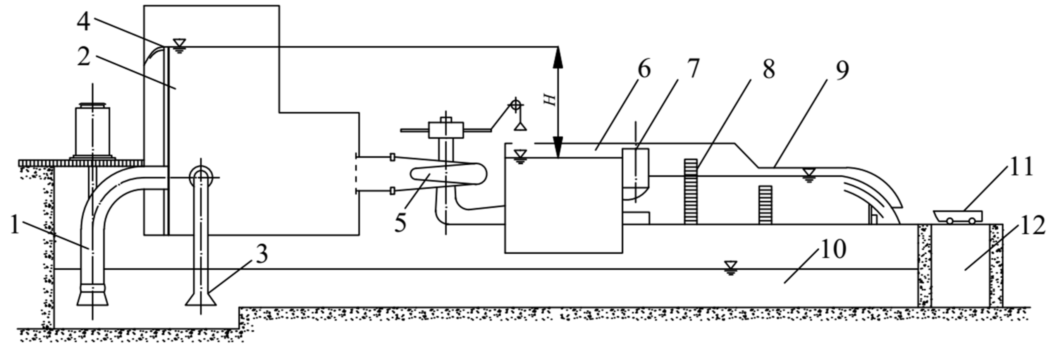
2.8. Experiment Apparatus

The Kaplan turbine model experiment on hydraulic transient process was performed on a dynamic hydro-mechanical experimental test rig at Hohai University. Figure 8 provides a computer-aided design (CAD) representation of the whole test loop.
The head of the test rig was measured using a pressure difference sensor with a precision of 0.1%; the pressure fluctuation was measured by pressure sensor with a precision of 0.6%; the discharge could be measured by electromagnetic flow meter or triangular weir, and the measuring accuracy was 0.3% and 0.15%, respectively. The stroke of guide vanes and blades were measured using a multi-circle helical potentiometer with a precision of 0.2%. The axial force of the turbine was measured using a tension-compression sensor and the resolution of axial force measurement was 0.1% of the rated load. The torque and rotational speed were measured using a torque-speed transducer which had a precision of 0.6% for torque and 0.5% for speed.

3. Results and Discussion

3.1. Comparison between Numerical and Experimental Results

To prove the accuracy and reliability of the numerical results of the load rejection process, the simulated runner rational speed and static pressure of the monitored points were compared with the experimental data [44], as shown in Figure 9. The numerical simulation results were generally in accordance with the experimental data on the overall trend. The simulated maximum rotational speed was 368.5 r/min, while the corresponding measured value was 362 r/min, showing only a 1.8% difference. Meanwhile, the discrepancy for n in some instances may be due to the relatively inaccurate turbulence model and low qualities of the dynamic mesh. In addition, the static pressure fluctuations for the three points between the two simulated and experimental results also showed some discrepancy: the simulated results presented lower pressure amplitudes at all three points. The discrepancies between the two methods may have been caused by the following reasons: some vibration signals may have interfered with the measured pressure results in the model experiment; the positions of the monitored points in the simulation were not completely identical to those in the actual dynamic test; the simulation and the experiment used two different sampling frequencies; the pressure tank was not established in the geometric model for the simulation, while the physical model contains a pipe system that also had an impact on the curves of the turbine, that is, the boundary condition was not completely consistent. Therefore, the numerical results could truly reflect the characteristics of the load rejection process only up to a certain degree.
The detail variations of static pressure obtained from CFD method for the three measured points are discussed next. The static pressure curve of point 1 declined slightly first, and then showed an upward trend since the flow was blocked when guide vanes started the closing process. The reason for the drop of the curve at the beginning was that the increase of the rotational speed resulted in an increase of the unit flux while the guide vanes had not begun to close yet, so a short negative water hammer appeared in the spiral casing. In the whole transient process, the pressure of point 1 fluctuated by a small amount and climbed steadily, and finally stabilized at around 8.0 kPa. For point 2, the fluctuation range of the static pressure was larger than those of the other two points, decreasing from 7.0 kPa to 2.8 kPa. The variation curve at point 2 had two trough values: 1.8 kPa at t = 2.35 s, which was close to the inflection point of the guide vanes’ closing law, since the guide vanes’ closing speed slowed down from that point on; 0.5 kPa at t = 6.3 s, which was near the completion of guide vanes’ closure as the water flow was totally cut off. The curve of point 3 showed that the pressure fluctuation in the draft tube was large during the transient process, which was caused by the complex outflow from the runner. Overall, the static pressure in the Kaplan turbine during the load rejection process demonstrated complex variability, not only affected by the dynamic parameters, but also related to the closure law of the regulating element.

3.2. The Varying Law of Dynamic Characteristic Parameters

To analyze the variation of each parameter with time, the dynamic values were compared with the initial values (Figure 10): runner blade opening φ0 = 15°, guide vanes’ opening (GVO) α0= 34.4°, unit mass flow rate Q0 = 0.233 m3/s, runner rotating speed n0 = 261 r/min, the initial torque M0 = 49.07 N·m, the initial axial force F0 = 627.86 N. Once the load rejection process began, the Kaplan turbine underwent the turbine mode and then the braking mode. In the beginning period, the unit was suddenly unloaded and the servomotor had a lag time after tripping, and the unit flow rate Q and the runner rotational speed n increased rapidly within the idle time of the guide vanes. From Figure 10a, when t = 0.3 s, the guide vanes began to close, the unit flow rate Q rose steadily and reached its peak at 0.75 s, which was 1.09 times the initial value. The Q curve experienced a similar “S” type decline from 0.8 s to the guide vanes segment point at t = 2.3 s as the guide vanes and blades started closing, the guide apparatus began to take over in place of the speed n to dominate the flow rate change. In particular, Q almost linearly fell below 2% of Q0.
The rotational speed n changed owing to the change of the torque. After the turbine entered the load rejection process, the plunge of the hydraulic moment caused the rise rate of n to drop and peaked at 369.2 r/min at 1.77 s, and the moment M (Figure 10b) passed through zero marked as a shift from turbine condition to braking condition. The hydraulic resistance moment shared a similar decreasing trend with the GVO curve from the beginning of braking mode to the segment point. After t = 2.3 s, the Q-curve’s decline rate started to slow down as the guide vanes’ closing speed reduced, and the hindering effect of the water flow on the runner rotation was reduced with the reduced resistance moment. When the Q dropped to around 30% of the Q0, the resistance moment kept an upward trend while the n curve went down at this stage. At 6.21 s, the flow was cut off due to the nearly closed guide vanes, and then the reversed moment M curve dipped with an inflection point.
In the simulation of the load rejection process, the maximum negative axial thrust is an important index for regulating guaranteed calculation. As plotted in Figure 10b, the variation curves of the axial force F and the moment M were consistent because their main source was the water thrust. However, the instant when the axial force F equaled zero was different from the instant when moment M was zero because the axial force has additional action surfaces from the hub and runner cone besides the blades. The maximum negative F with a relative value of −0.638 occurred when the guide vanes were nearly closed. All the dynamic parameters gradually stabilized when the blades finished the closing process.

3.3. Analysis of Flow Characteristics

Generally, the variations of dynamic parameters are the external expression of intrinsic flow field evolution, which will lead to changes of a turbine’s mechanical property. Thus, the internal flow state in a Kaplan turbine passage will present different characteristics during a load-rejection transient process. The flow configuration in different parts of turbine passage at some critical moments was visualized for analysis.
The velocity vector on the surface at half the height of the stay vanes and guide vanes at different time are displayed in Figure 11. The initial condition showed a perfect performance with no influx and backflow, and the velocity distribution around the stay vanes and guide vanes was uniform (Figure 11a). After the load rejection process began, with the closing of the guide vanes, a large velocity contour and flow separation between adjacent guide vanes were observed (Figure 11b–f). At the guide vanes’ closing inflection point (t = 2.3 s), the flow was still uniform as the flow angle in front of the guide vanes was almost unchanged, and at this time, the guide vanes’ openings were decreased by 60%. In addition, the circumferential velocity of the water flow behind the guide vanes increased because of the noticeable flow impact between the adjacent guide vanes, owing to the smaller GVO. When the guide vanes were 96% closed at t = 5.8 s (Figure 11f), the mass flow rate Q had dropped to 9% of Q0 and the flow in the spiral casing almost stopped with only a little flow present in the gap between the guide vanes. After the guide vanes were closed (Figure 11g–i), the water flow was blocked and the flow regime in the passage between the stay vanes became chaotic. The upstream side also formed a small amount of reflux between the stay vanes and the guide vanes. Simultaneously, a circumfluent flow with a low velocity were formed between guide vanes and stay vanes as a result of the previous flow inertia.
The runner is the most important part of a Kaplan turbine and its flow pattern development has a great effect on the transient process and steady-state conditions for the whole hydropower station. The pressure contour on the blades and the velocity vector on the two typical sections (shown as Figure 2) are provided in Figure 12 and Figure 13, respectively. As expected, there was no bad flow pattern in the runner region (Figure 12a) in the beginning condition, and the gradient distribution of the flow velocity was homogeneous (Figure 13a). Once load rejection happened, with the change of the rotational speed and mass flow rate, the flow pattern in the runner would be complex and unsteady. When the runner rotational speed n reached its peak value at t = 1.76 s, there was a negative pressure region near the inlet edge of the runner tip because the gradual decline of the relative flow angle with n rose on the blade inlet edge, where some flow impacts occurred (Figure 12b), and thus resulted in flow separation and significant energy dissipation (Figure 13b). After that, the flow rate Q underwent a sharp decline, but the runner speed was high. As a result, the water flow shrank from the guide vanes into the runner chamber and was subjected to centrifugal forces, which would lead to a majority of the flow moving outward and a large negative pressure area on the runner hub and cone (Figure 12c). After that, the static pressure on the runner hub and cone rose a bit and the pressure on the blade surface consistently became more uniform (Figure 12d–g). Furthermore, the circulating component of the runner inflow would climb and backflow appeared on the runner cone surface, which was the main source of a reverse thrust. Some high-speed circulation appeared due to the impact of the partial stall flow striking against the blades, which experienced acceleration, convergence with the low velocity flow, and deceleration. After the guide vane was completely closed, the impeller flow was blocked, and the flow instability was increased by a backflow vortex at the outlet edge of the middle section of the blade (Figure 13e–f).
As the draft tube was directly connected with the runner, its internal flow pattern was complex. According to Figure 14a, the initial flow regime in the draft tube was homogeneous before load rejection happened. There were five low pressure zones in the draft tube’s inlet section, which was affected by the impeller flow. Similarly, the inlet flow was disturbed by blades and formed five clockwise rotating vortex zones, which extended to the straight cone section. With the rotational speed n increasing, the static pressure at the inlet center of the draft tube fell to its lowest point (−3 kPa) when n reached its peak and deviated greatly from the circular center of the inlet section (Figure 14b). During the first stage of the guide vanes’ closure, the flow velocity was uneven when water flowed through the elbow section and the streamlines in the diffuser portion were extremely chaotic. At the upstream side of the draft tube wall, there was a low-velocity stagnating flow area caused by the impingement of the flow and the upstream wall while the downstream flow shrank and accelerated, leading to a large negative pressure area on the passage wall upstream; therefore, the main water flow migrated toward the wall downstream due to the pressure differences (Figure 14c). Between t = 4.8 s and t = 6.4 s, the static pressure of the draft tube wall increased, owing to the continuous impact between the draft tube wall and the annular inflow dominated by the minimal GVO. When the flows reached the bottom of the elbow section, there were two flow patterns. One is the mainstream which hit the wall and bounced back into backflows, and the other is the remaining spiral outflow that flows out along the upper passage behind the support pier while the rest of the passage became stagnant water area. At the end of the load rejection process, the unit flux almost equaled to zero, and the streamlines became very disordered while the pressure gradient was very small. Simultaneously, the flow in the draft tube was only driven by the runner and the rotational inertia, which changed little after the transient process.

4. Conclusions

In this study, a 3-D numerical simulation of the load rejection process of a Kaplan turbine based on co-adjustments of the guide vanes and runner blades was performed using a dynamic mesh method. The simulated results of the rotational speed and static pressure variations at the monitored points agreed well with the experimental data of the corresponding dynamic model. The error for the maximum speed during the transient process was only 1.8%. The variation regularity of the unit rotational speed n, mass flow rate Q, moment M and axial thrust F with time were revealed during the load rejection transient, which can provide useful references for turbine structure designs and operations. Moreover, the time-varying pressure fluctuations were recorded to capture the water hammer. Based on the CFD results, the flow fields and the unsteady flow evolution were analyzed in detail for the whole transient process.
The external characteristic changes were dominated by the guide vane closing while the runner blades’ closure had marginal influence on them. Especially, the moment M, axial force F, and static pressure at point 2 all had two troughs at the inflection point of the guide vanes’ closure curve. The peak value of the rotation speed was 368.5 r/min, which was 1.41 times the initial value n0. The maximum negative axial force was 0.638 times F0 and occurred at the end of the guide vanes closing, which means that the closing time of the guide vanes could be extended to avoid the hang-up risks of the Kaplan turbine. The pressure variation range at point 2, which was near the runner inlet, was larger and the pressure fluctuation at point 3, which was close to runner outlet, was intense. Therefore, the dynamic rotor-stator interactions had a great influence on the static pressure. Furthermore, the flow pattern in the unit passage varied dramatically, especially in the proximity of the inflection point. There were severe vortex and reflux at the runner with local high and low pressure on the blade surfaces, which may lead to cavitation, and an apparent water hammer appeared at the guide vanes. Flow swirling in the draft tube was serious and the static pressure on the wall fell suddenly, which could incur strong low frequency pressure fluctuations and unit vibrations. Thus, the most important moment during the process was determined to be the segment point of guide vanes’ closing law, which may be reasonably controlled to effectively reduce the influence of a water hammer on the turbine’s dynamic characteristics.
Future studies could also consider the water density change during the transient process, which may also have an impact on the results. Furthermore, the calculation conditions should be increased for different opening and closure laws for the guide vanes and the blades to investigate the load-rejection transient process more precisely. In the future work, the whole flow system including upstream and downstream reservoirs should be established, the gravity term should be added, and the boundary conditions should be modified, so that more precise and comprehensive flow characteristics can be investigated during the transient process of the Kaplan turbine.

Author Contributions

H.C. performed the numerical simulation, analyzed the numerical results, and wrote the paper; D.Z. provided the experimental data and wrote the paper; Y.Z. and A.Y. suggested the methodology and provided valuable advice; S.J. and Y.G. designed the numerical methods and performed the calculations.

Funding

The study was financially supported by the National Natural Science Foundation of China (No.51339005, No.51839008, No.51806058), the Fundamental Research Funds for the Central Universities (2016B41514), and the Chinese Scholarship Council (No.201606710029). The study was also supported by the Open Research Fund Program of State Key Laboratory of Water Resource and Hydropower Engineering Science (2015SDG04).

Acknowledgments

The authors would like to acknowledge the financial support of Hohai University and Chinese Scholarship Council, China. Many thanks to the valuable suggestions and manuscript revisions of Huidong Li from Pacific Northwest National Laboratory, USA.

Conflicts of Interest

The authors declare no conflict of interest.

Nomenclature

CBoundary moving velocitym/s
DRunner diameterm
d S Infinitesimal aream2
FAxial forceN
F0Initial axial forceN
gGravitational body forcem/s2
JTotal unit moment of inertiakg·m2
MMoment of the rotational systemN·m
M0Initial torqueN·m
mOutward normal unit vector-
nRunner rotating speedr/min
n0Initial runner rotating speedr/min
PStatic pressureMPa
QUnit flow ratem3/s
Q0Initial unit flow ratem3/s
tTimes
uFluid velocitym/s
VVolume of control bodym3
wGrid velocitym/s
α 0 Initial guide vanes opening°
α Guide vanes opening°
φ 0 Initial runner blade opening°
φ Runner blade opening°
θ Rotational angle of the blade around the axis°
ω Angular velocity vectorrad/s
ω B Closing speed of runner bladerad/s
ω x Angular velocity components of runner blade in the x -axis directionrad/s
ω y Angular velocity components of runner blade in the y -axis directionrad/s
ω z Angular velocity components of runner blade in the z -axis directionrad/s
ω G V Closing speed of guide vanesrad/s
μMolecular viscosityPa·s
ρDensity of fluidkg/m3
Δ t Time step sizes
Hamilton operator-
2 Laplacian operator-
Ω Boundary of control volume-

Abbreviations

3-DThree-dimensional
ALEArbitrary Lagrangian Eulerian
CFDComputational fluid dynamics
FVMFinite volume method
GVOGuide vanes’ opening
NMECNumerical method of external character
NMICNumerical method of internal character
RANSReynolds-averaged Navier–Stokes
SIMPLECSemi-implicit method for pressure-linked equations—consistent
SPSingle phase
SST k ω Shear-stress transport k ω turbulence model
UDFUser defined function
VOFVolume of fluid

References

  1. Zhou, D.; Deng, Z. Ultra-low-head hydroelectric technology: A review. Renew. Sustain. Energy Rev. 2017, 78, 23–30. [Google Scholar] [CrossRef]
  2. Elbatran, A.; Yaakob, O.; Yasser, M.; Shabara, H. Operation, performance and economic analysis of low head micro-hydropower turbines for rural and remote areas: A review. Renew. Sustain. Energy Rev. 2015, 43, 40–50. [Google Scholar] [CrossRef]
  3. Bozhinova, S.; Hecht, V.; Kisliakov, D.; Müller, G.; Schneider, S. Hydropower converters with head differences below 2.5 m. Proc. Inst. Civ. Eng. Energy 2013, 166, 107–119. [Google Scholar]
  4. Jawahar, C.; Michael, P. A review on turbines for micro hydro power plant. Renew. Sustain. Energy Rev. 2017, 72, 882–887. [Google Scholar] [CrossRef]
  5. Senior, J.; Saenger, N.; Müller, G. New hydropower converters for very low-head differences. J. Hydraul. Res. 2010, 48, 703–714. [Google Scholar] [CrossRef]
  6. Zhou, D.; Wu, Y.; Mao, Y. Three dimensions unsteady CFD simulation of model propeller turbine load rejection transient. In Proceedings of the ASME 2010 International Mechanical Engineering Congress & Exposition, Vancouver, BC, Canada, 12–18 November 2010. [Google Scholar]
  7. Li, J.; Yu, J.; Wu, Y. 3D unsteady turbulent simulation of transients of the Francis turbine. In IOP Conference Series: Earth and Environmental Science; IOP Publishing: Bristol, UK, 2010; Volume 12, p. 012001. [Google Scholar]
  8. Kolšek, T.; Duhovnik, J.; Bergant, A. Simulation of unsteady flow and runner rotation during shut-down of an axial water turbine. J. Hydraul. Res. 2006, 44, 129–137. [Google Scholar] [CrossRef]
  9. Rohani, M.; Afshar, M. Simulation of transient flow caused by pump failure: Point-implicit method of characteristics. Ann. Nucl. Energy 2010, 37, 1742–1750. [Google Scholar] [CrossRef]
  10. Wu, R.; Chen, J. Hydraulic Transient Process of Hydropower Station; China Water & Power Press: Beijing, China, 1995. [Google Scholar]
  11. Gajic, A. Steady and Transient Regimes in Hydropower Plants. In IOP Conference Series: Materials Science and Engineering; IOP Publishing: Bristol, UK, 2013; Volume 52, p. P012006. [Google Scholar]
  12. Zhao, J.; Wang, L.; Liu, D.; Wang, J.; Zhao, Y.; Liu, T.; Wang, H. Dynamic model of Kaplan turbine regulating system suitable for power system analysis. Math. Probl. Eng. 2015, 2015, 294523. [Google Scholar] [CrossRef]
  13. Chirag, T.; Cervantes, M.J.; Bhupendrakumar, G.; Dahlhaug, O.G. Pressure measurements on a high-head Francis turbine during load acceptance and rejection. J. Hydraul. Res. 2014, 52, 283–297. [Google Scholar] [CrossRef]
  14. Chirag, T.; Agnalt, E.; Dahlhaug, O.G. Experimental investigation of a Francis turbine during exigent ramping and transition into total load rejection. J. Hydraul. Eng. 2018, 144, 04018027. [Google Scholar]
  15. Hasmatuchi, V.; Farhat, M.; Roth, S.; Botero, F.; Avellan, F. Experimental evidence of rotating stall in a pump-turbine at off-design conditions in generating mode. J. Fluids Eng. 2011, 133, 051104. [Google Scholar] [CrossRef]
  16. Gagnon, M.; Jobidon, N.; Lawrence, M.; Larouche, D. Optimization of turbine startup: Some experimental results from a propeller runner. In IOP Conference Series: Earth and Environmental Science; IOP Publishing: Bristol, UK, 2014; Volume 22, p. 032022. [Google Scholar]
  17. Chirag, T.; Gogstad, P.J.; Dahlhaug, O.G. Investigation of the unsteady pressure pulsations in the prototype Francis turbines during load variation and startup. J. Renew. Sustain. Energy 2017, 9, 0645802. [Google Scholar]
  18. Yang, J.; Zeng, W.; Yang, W.; Yao, S.; Guo, W. Runaway stabilities of pump-turbines and its correlation with S characteristics curves. Trans. Chin. Soc. Agric. Mach. 2015, 46, 59–64. [Google Scholar]
  19. Liu, Y.; Chang, J. Numerical method based on internal character for load rejection transient calculation of a bulb turbine installation. J. China Agric. Univ. 2008, 13, 89–93. [Google Scholar]
  20. Chirag, T.; Agnalt, E.; Dahlhaug, O.G. Numerical techniques applied to hydraulic turbines: A perspective review. Appl. Mech. Rev. 2016, 68, 010802. [Google Scholar]
  21. Pejovic, S.; Karney, B. Guidelines for transients are in need of revisions. In IOP Conference Series: Earth and Environmental Science; IOP Publishing: Bristol, UK, 2014; Volume 22, p. 042006. [Google Scholar]
  22. Pavesi, G.; Cavazzini, G.; Ardizzon, G. Numerical analysis of the transient behaviour of a variable speed pump-turbine during a pumping power reduction scenario. Energies 2016, 9, 534. [Google Scholar] [CrossRef]
  23. Zhang, L.; Zhou, D. CFD research on runaway transient of pumped storage power station caused by pumping power failure. In IOP Conference Series: Materials Science and Engineering; IOP Publishing: Bristol, UK, 2013; Volume 52, p. 052027. [Google Scholar]
  24. Liu, S.; Zhou, D.; Liu, D.; Wu, Y.; Nishi, M. Runaway transient simulation of a model Kaplan turbine. In IOP Conference Series: Earth and Environmental Science; IOP Publishing: Bristol, UK, 2010; Volume 12, p. 012073. [Google Scholar]
  25. Liu, J.; Liu, D.; Sun, Y.; Jiao, L.; Wu, Y.; Wang, L. Three-dimensional flow simulation of transient power interruption process of a prototype pump-turbine at pump mode. J. Mech. Sci. Technol. 2013, 27, 1305–1312. [Google Scholar] [CrossRef]
  26. Liu, J.; Liu, S.; Sun, Y.; Wu, Y.; Wang, L. Three-dimensional flow simulation of load rejection of a prototype pump-turbine. Eng. Comput. 2013, 29, 417–426. [Google Scholar]
  27. Avdyushenko, A.; Cherny, S.; Chirkov, D.; Skorospelov, V.; Turuk, P. Numerical simulation of transient processes in hydro-turbines. Thermophys. Aeromech. 2013, 20, 577–593. [Google Scholar] [CrossRef]
  28. Fu, X.; Li, D.; Wang, H.; Zhang, G.; Li, Z.; Wei, X. Analysis of transient flow in a pump-turbine during the load rejection process. J. Mech. Sci. Technol. 2018, 32, 2069–2078. [Google Scholar] [CrossRef]
  29. Fu, X.; Li, D.; Wang, H.; Zhang, G.; Li, Z.; Wei, X.; Qin, D. Energy analysis in a pump-turbine during the load rejection process. J. Fluids Eng. 2018, 140, 101107. [Google Scholar] [CrossRef]
  30. Nicolle, J.; Morissette, J.; Giroux, A. Transient CFD simulation of a Francis turbine startup. In IOP Conference Series: Earth and Environmental Science; IOP Publishing: Bristol, UK, 2012; Volume 15, p. 062014. [Google Scholar]
  31. Nicolle, J.; Giroux, A.; Morissette, J. CFD configurations for hydraulic turbine startup. In IOP Conference Series: Earth and Environmental Science; IOP Publishing: Bristol, UK, 2014; Volume 22, p. 032021. [Google Scholar]
  32. Li, Y.; Song, G.; Yan, Y. Transient hydrodynamic analysis of the transition process of bulb hydraulic turbine. Adv. Eng. Softw. 2015, 90, 152–158. [Google Scholar] [CrossRef]
  33. Li, D.; Wang, H.; Li, Z.; Nielsen, T.; Goyal, R.; Wei, X.; Qin, D. Transient characteristics during the closure of guide vanes in a pump turbine in pump mode. Renew. Energy 2018, 118, 973–983. [Google Scholar] [CrossRef]
  34. Zhou, D.; Chen, H.; Zhang, L. Investigation of pumped storage hydropower power-off transient process using 3D numerical simulation based on SP-VOF hybrid model. Energies 2018, 11, 1020. [Google Scholar] [CrossRef]
  35. Yakhot, V.; Orszag, S. Renormalization group analysis of turbulence. I Basic theory. J. Sci. Comput. 1986, 1, 3–51. [Google Scholar] [CrossRef]
  36. Rentschler, M.; Marongiu, J.; Neuhauser, M.; Parkinson, E. Overview of SPH-ALE applications for hydraulic turbines in ANDRITZ hydro. J. Hydrodyn. 2018, 30, 114–121. [Google Scholar] [CrossRef]
  37. Zhou, D.; Zhang, L. CFD research on Francis pump-turbine load rejection transient under pump condition. In Proceedings of the ASME 2013 International Mechanical Engineering Congress & Exposition, San Diego, CA, USA, 15–21 November 2013. [Google Scholar]
  38. Menter, F.; Rumsey, C. Assessment of two-equation models for transonic flows. In Proceedings of the Fluid Dynamics Conference, Colorado Spring, CO, USA, 20–23 June 1994; pp. 1994–2343. [Google Scholar]
  39. Kan, K.; Zheng, Y.; Chen, Y.; Xie, Z.; Yang, G.; Yang, C. Numerical study on the internal flow characteristics of an axial-flow pump under stall conditions. J. Mech. Sci. Technol. 2018, 32, 4683–4695. [Google Scholar] [CrossRef]
  40. Ansys Inc. Ansys FLUENT Theory Guide; Ansys Inc.: Canonsburg, PA, USA, 2017. [Google Scholar]
  41. Menter, F. Two-equation eddy-viscosity turbulence models for engineering applications. AIAA J. 1994, 32, 1598–1605. [Google Scholar] [CrossRef] [Green Version]
  42. Kan, K.; Zheng, Y.; Fu, S.; Liu, H.; Yang, C.; Zhang, X. Dynamic stress of impeller blade of shaft extension tubular pump device based on bidirectional fluid-structure interaction. J. Mech. Sci. Technol. 2017, 31, 1561–1568. [Google Scholar] [CrossRef]
  43. Murayama, M.; Nakahashi, K.; Maltsushima, K. Unstructured dynamic mesh for large movement and deformation. In Proceedings of the 40th Aerospace Science Meeting and Exhibit, Reno, NV, USA, 14–17 January 2002; p. AIAA2002-0122. [Google Scholar]
  44. Hohai University, Gezhouba Hydropower Plant. Dynamic Model Test Report on Transient Process of ZZ500 Turbine in Gezhouba Hydropower Plant; Hohai University: Nanjing, China, 1992. [Google Scholar]
Figure 1. Algorithm routines of the load rejection transient simulation.
Energies 11 03354 g001
Figure 2. Sketch of the entire computational domain for the Kaplan turbine model.
Energies 11 03354 g002
Figure 3. Monitoring points of static pressure in the whole passage.
Energies 11 03354 g003
Figure 4. (a) Closing process of the guide vanes, (b) t = 0 s, (c) t = 2.2 s, (d) t = 4.2 s, and (e) t = 6.3 s.
Energies 11 03354 g004
Figure 5. (a) Closing process of the blades, (b) t = 0 s, (c) t = 4.2 s, (d) t = 6.4 s, and (e) t = 9.2 s.
Energies 11 03354 g005
Figure 6. Test results of the three different mesh schemes.
Energies 11 03354 g006
Figure 7. Pre-calculated results of different time step size.
Energies 11 03354 g007
Figure 8. The CAD representation of the test loop, where 1-pump, 2-head tank, 3-bypass valve, 4-overflow plate, 5-Kaplan turbine model, 6-draft tank, 7-regulating grid, 8-stabilizing grid, 9-flow measuring flume, 10-collecting basin, 11-closure trolley, and 12-flow rate calibration slot.
Energies 11 03354 g008
Figure 9. Curves of numerical simulation and experiment results.
Energies 11 03354 g009
Figure 10. Variation of normalized dynamic parameters in the load rejection process, (a) the variations of runner rotate speed and unit flow rate, (b) the variations of moment and axial force.
Energies 11 03354 g010
Figure 11. Velocity vector between stay vanes and guide vanes at different time: (a) t = 0 s, (b) t = 1.76 s, (c) t = 2.3 s, (d) t = 3.2 s, (e) t = 4.8 s, (f) t = 5.8 s, (g) t = 6.4 s, (h) t = 7.0 s, and (i) t = 9.2 s.
Energies 11 03354 g011
Figure 12. Distribution of the velocity vector and static pressure in the runner zone at different time: (a) t = 0 s, (b) t = 1.76 s, (c) t = 2.3 s, (d) t = 3.2 s, (e) t = 4.8 s, (f) t = 5.8 s, (g) t = 6.4 s, (h) t = 7.0 s, and (i) t = 9.2 s.
Energies 11 03354 g012
Figure 13. Velocity vector distribution on Span 1 (upper) and Span 2 (lower) at different time: (a) t = 0 s, (b) t = 1.76 s, (c) t = 3.2 s, (d) t = 4.8 s, (e) t = 6.4 s, and (f) t = 7.0 s.
Energies 11 03354 g013
Figure 14. Flow fields in the draft tube at different time: (a) t = 0 s, (b) t = 1.76 s, (c) t = 2.3 s, (d) t = 4.8 s, (e) t = 6.4 s, and (f) t = 9.2 s.
Energies 11 03354 g014
Table 1. Main parameters of the Kaplan turbine model.
ParametersValue
Diameter of runner (m)0.46
Number of runner blades (-)5
Number of guide vanes (-)32
Number of stay vanes (-)16
Height of guide vanes (m)0.184
Runner blade rated opening (°)15
Guide vane rated opening (°)41.55
Rated head of turbine (m)0.82
Rated speed of turbine (r/min)261
Rated discharge of turbine (m3/s)0.33
Total unit moment of inertia (kg·m2)16.8
Specific speed of the turbine (-)500

