A New Reservoir Operation Chart Drawing Method Based on Dynamic Programming

Abstract

A reservoir operation chart is an important tool in guiding actual reservoir operation at present. There are mainly two kinds of methods in drawing the operation chart, i.e., conventional methods and optimization methods, but each of them has some shortcomings, such as the repeated empirical inspection and correction of conventional methods, and the sensitivity to the initial trajectories of some optimization algorithms. In view of this, based on the principle of dynamic programming (DP), this paper coupled the reservoir operation chart drawing model and the DP model, and proposed a new reservoir operation chart drawing method which has no empirical inspection and correction, no requirement for initial solution, no problem of premature convergence and local convergence. In addition, this method can guarantee the global convergence of the results to a certain extent because of the global convergence of DP. Ya Yangshan reservoir in the Li Xianjiang River of China was selected as the research object to derive the operation chart by the drawing method. The simulation results show that the proposed method in this paper presents better performance compared with the conventional method on power generation, guaranteed output, and assurance rate, especially on the latter, which has a 2.68% increase. In addition, compared with the deterministic optimization results of DP, it is found that the results of the proposed method are very close to that of deterministic DP, the differences are only 1.8 GWh (0.36% decline) and 1.6 GWh (0.32% decline). So, the validity and rationality of the proposed method are further verified by the simulation results.

1. Introduction

As one of the clean energy sources, hydropower energy is the most important renewable source for generation of electricity worldwide and can be developed on a large-scale [1,2]. It can reduce the use of fossil fuels for electricity generation, and reduce worldwide CO₂-emmissions. Hydropower contributed 16.5% to the world electricity generation in 2012, while the other renewables contributed only 5.2% [3]. Compared with other energy sources, hydropower enjoys exceptional advantages [4,5] which are clean, pollution-free, quick in output, and can quickly adapt to load changes of power system [6]. In addition, water is the main input for hydropower station to produce the electricity [7], and it is present and usable all over the year in contrast to wind and solar that are intermittent technologies and only usable when these resources are available, so hydropower energy is a superior sustainable energy source to help maintain sustainable growth and quality of life [8]. These advantages of hydropower mean that reservoir operation optimization research has the attention of many scholars all over the world [9,10,11]. However, in the actual long- and mid-term reservoir operation, operation rules are needed because of the inflow uncertainties and forecasting level [12,13]. It is realistic to get the satisfactory solution via pre-obtained operation rules [14,15].

Reservoir operation rules are varied [16,17,18], and an often-used rule is the reservoir operation chart nowadays. A reservoir operation chart is the graphical result of operation rules, and it contains three main kinds of operation curves and operation zones. Direct and concise is the notable feature of reservoir operation chart, the reservoir operation decision made by the operation chart is well in accord with the operation principle. At present, the reservoir operation chart has been widely applied in actual production.

At present, there are mainly two kinds of methods to derive the reservoir operation chart, the first one is the conventional method, in which the reservoir operation chart can be obtained by a reverse calculation, and the runoff data of typical years is used in this calculation. Specific steps of conventional methods can be found in the literature by Shao et al. [19] and Yu et al. [20]. The calculated operation chart can ensure the normal operation of reservoir in most situations, and it has a clear physical meaning and high reliability. Thus, achieves different degrees of success in different reservoirs. However, it has some disadvantages, such as repeated empirical inspection and correction with high complexity and randomicity [21].

The second method is the optimization method, which usually optimizes the operation curves based on an obtained initial solution. Many optimization algorithms were used to optimize the reservoir operation chart in the past decades [22,23], such as genetic algorithm (GA) [24,25], particle swarm optimization (PSO) [26,27], and progressive optimality algorithm (POA) [28,29]. It is relatively simple and easy to gain the reservoir operation chart through various optimization algorithms. However, there are also some disadvantages. First of all, they usually have the requirements for the initial curves, and they can only implement the simulation optimization for the initial curves, and cannot figure out the optimal operation chart directly, furthermore, the quality of the provided initial solution has a great influence on the final results [30]. Secondly, it is very hard to achieve a global optimal solution, although it has been proven that many evolutionary algorithms have a global convergence, they cannot ensure a global optimal solution within finite iteration calculations as these algorithms are affected by stochastic feature [31]. Thirdly, some optimization methods (such as POA) impose the restrictions on the unsmooth and non-convex nature of the problems. The main advantages and disadvantages of these optimization algorithms can be simply summarized as shown in

Table 1. Advantages and disadvantages of each optimization algorithms

Algorithms	Is the Initial Solution Needed?	Is It Random?	Is There Any Requirement for Unsmooth and Non-Convex?	Is It Possible to Get the Global Optimal Solution?	Computing Time
GA, PSO	Initial population needed	Yes	No	Difficult because of randomness	Short
POA	An initial solution needed	No	Yes	Greatly influenced by initial solution	Short
DP	Do not need	No	No	Yes	Long

.

Dynamic programming (DP) is a powerful optimization technique [32,33], and the most striking feature of DP is that it can ensure the global optimum and no initial solution is needed. Besides, DP has no requirements on non-convex and unsmooth nature of the optimization problems. This makes DP obtain a high popularity in the classical optimization algorithms [34]. However, although many methods were used to optimize the reservoir operation chart as mentioned above, DP was rarely used to derive the reservoir operation chart directly. Therefore, the optimality of DP has not been well applied to the reservoir operation chart optimization.

In view of this, the reservoir operation chart drawing model and the DP model are coupled in this research, and this paper proposed a new reservoir operation chart drawing method based on DP. Compared with the conventional drawing method, it is more direct and effective to directly calculate the optimal operation chart through the DP model, and there is no repeated empirical inspection and correction. Compared with other optimization algorithms, there is no requirement for an initial solution, and there is no problem with premature convergence and local convergence too. In addition, the proposed method can guarantee the global convergence of the results to a certain extent because of the global convergence of DP. The remaining parts are organized as follows in this paper. Section 2 will present the drawing model of reservoir operation chart based on DP, including the specific calculation process and the detailed steps in the actual application. Section 3 will show the case study of Ya Yangshan reservoir in Li Xiangjiang River, and the results will be presented and analyzed in Section 3.2. Finally, the conclusions of this paper will be summarized and provided in Section 4.

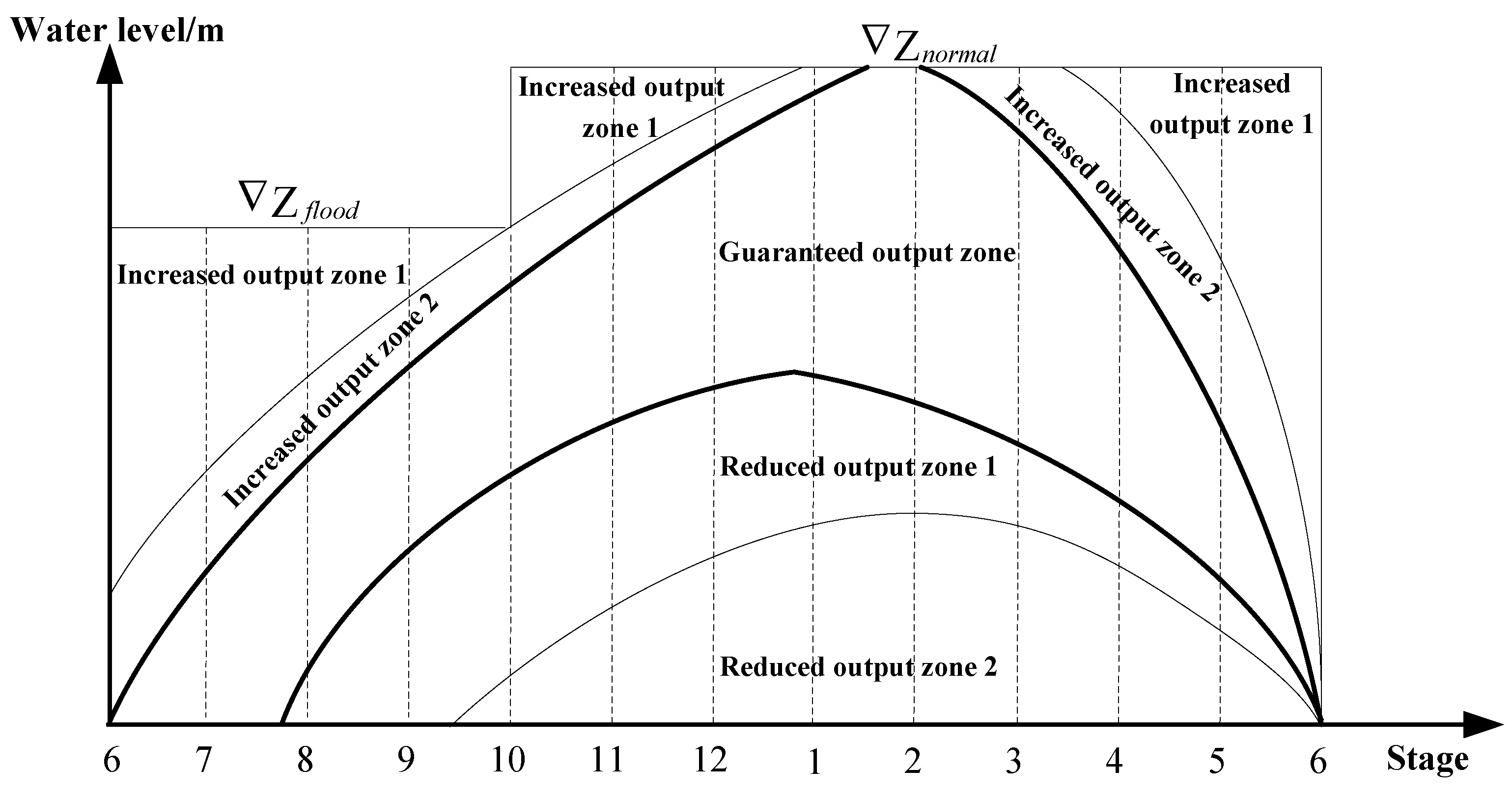
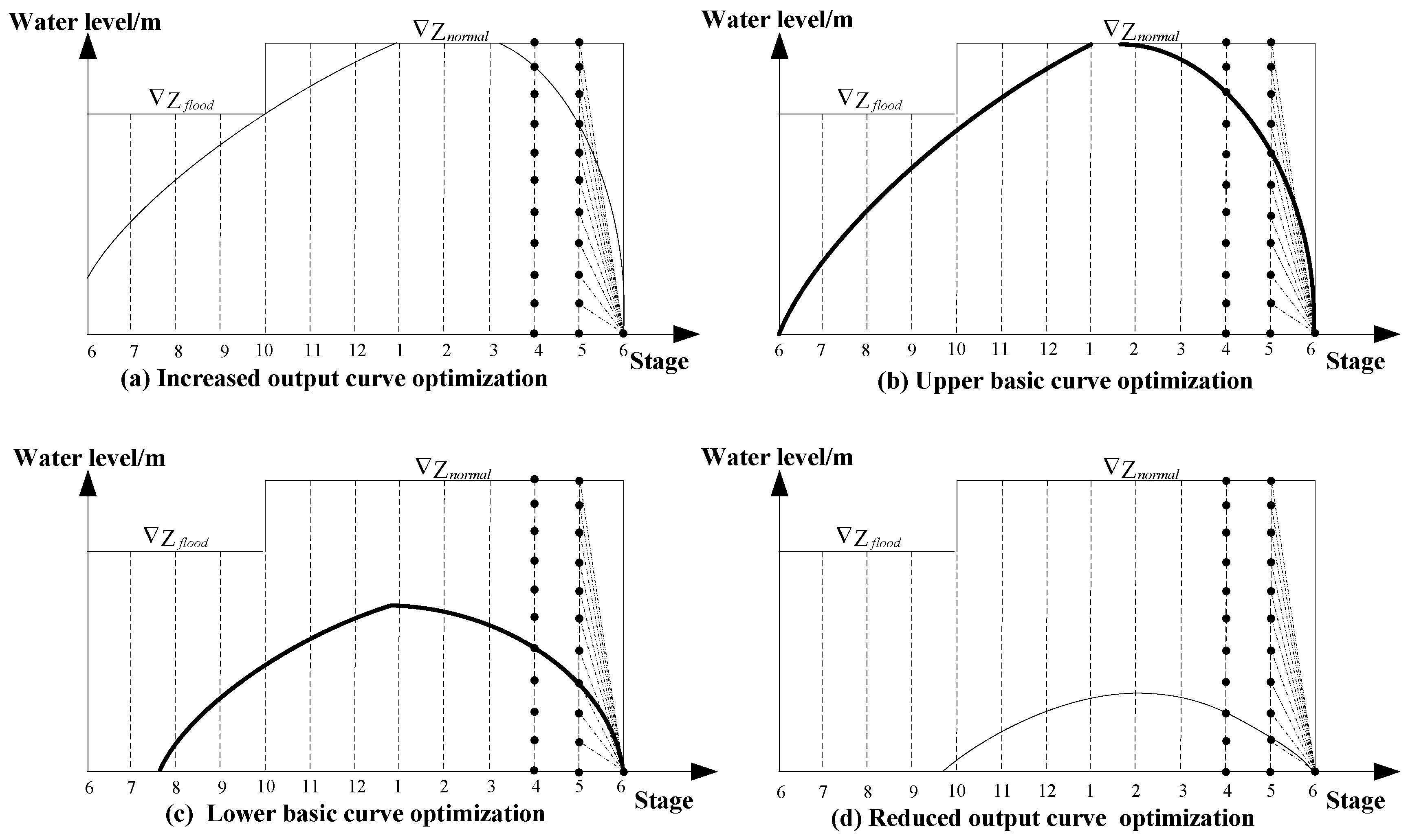
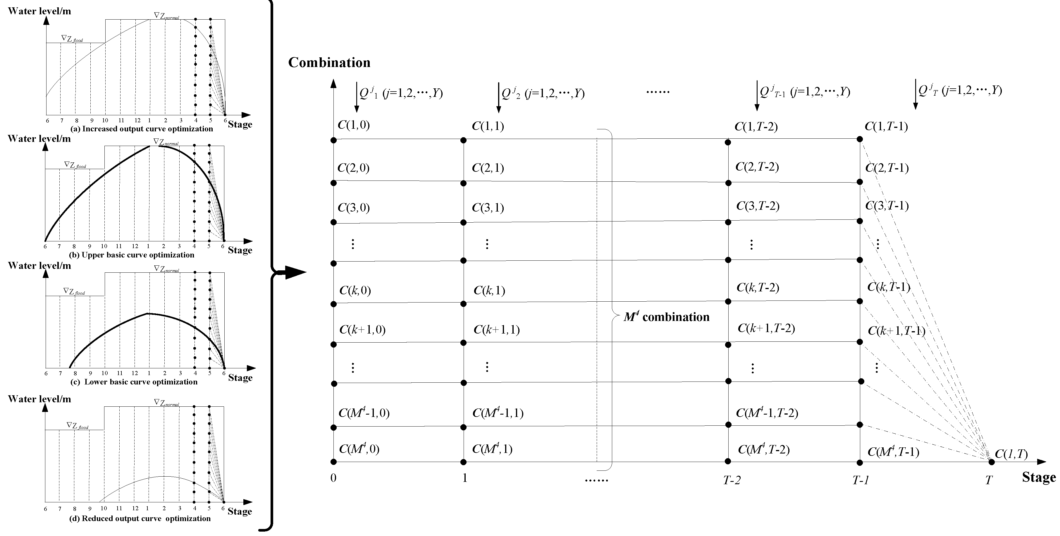
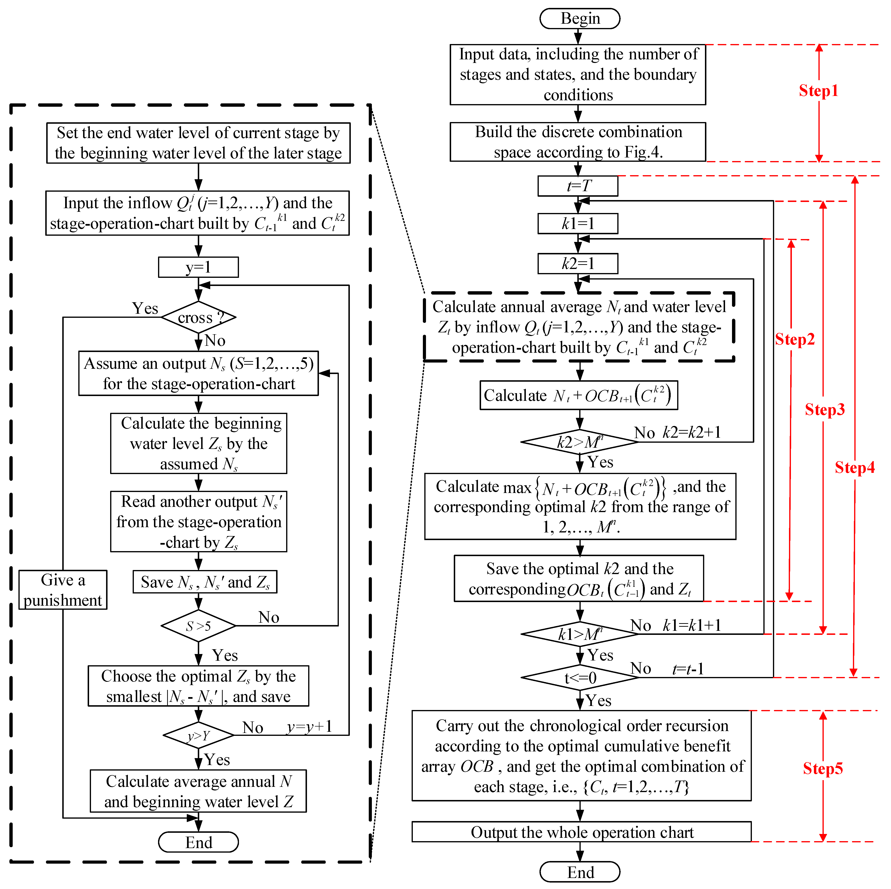
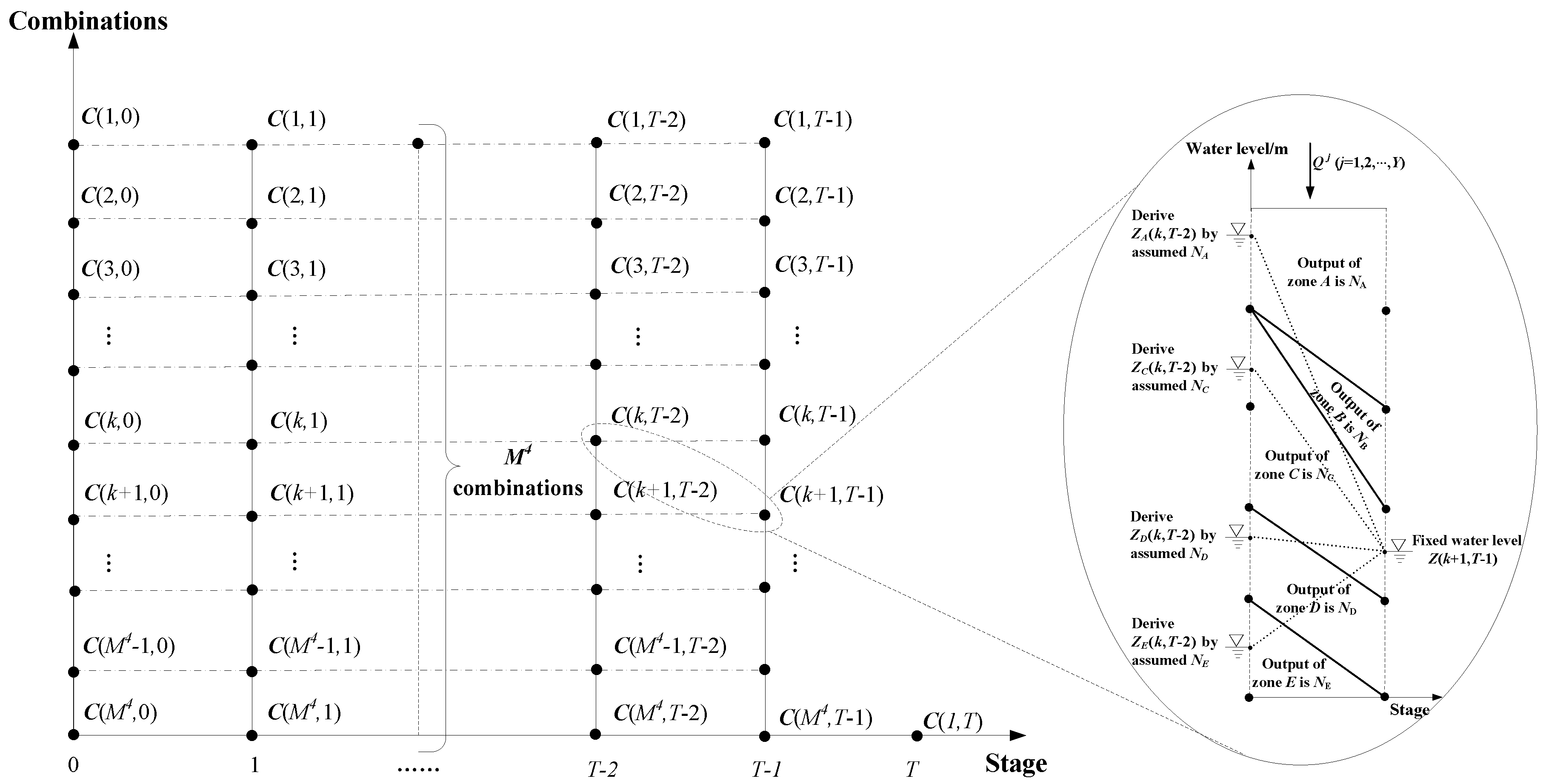
2. DP Based Reservoir Operation Chart Drawing Model

There are three types of output in the actual hydropower station dispatching, i.e., guaranteed output, increased output, and reduced output. Correspondingly, there are three kinds of operation zones in the operation chart, which are the guaranteed output zone, the increased output zone and the reduced output zone. So, there are three types of operation curves in a reservoir operation chart, i.e., the basic operation curves (including the upper and lower basic operation curve), the increased output curves, and the reduced output curves. The upper basic operation curve and lower basic operation curve corresponds to the upper and lower boundary of guaranteed output zone.

The conventional reservoir operation chart is shown in Figure 1, in which the number of the increased and the reduced output curves can be more than one according to the needs. Here, for the simplified representation, only one increased output curve and one reduced output curve are provided. In Figure 1, the abscissa axis represents the time (month), and the ordinate axis represents the reservoir water level whose upper limit is the flood control level in the flood season the normal storage level in the non-flood season [35]. The curves in Figure 1 from top to bottom are in turn the increased output curve, the upper basic curve, the lower basic curve and the reduced output curve. These curves divide the whole dispatching map area into several corresponding output zones. The detailed process of how to use the DP model to directly calculate the optimal reservoir operation chart will be described in the following.

Firstly, separate the four curves in Figure 1 and place them in four separated coordinates, and get the feasible water level range of each operation curve, and discretize it, as shown in Figure 2. Figure 2a represents that the increased output curve in Figure 1 is taken out separately and placed in a separate coordinate system. Figure 2b represents that the upper basic operation curve in Figure 1 is taken out separately and placed in a separate coordinate system. Figure 2c,d have similar meanings to Figure 2a,b.

Secondly, from Figure 2, it can be seen that, corresponding to each discretized water level point of the basic operation curves, the increased output curve and the reduced output curve at the beginning of a stage, a water level combination can be obtained, and another similar combination by the discretized water level points of each curve at the end of this stage can be obtained too. The two combinations can constitute a stage-operation-chart if their position relationship is satisfied (no cross), as shown in Figure 3.

All the possible discretized water level combinations of the four operation curves over the whole operation period are shown in Figure 4, where C(k, t) represents the kth combination in the tth stage, k = 1, 2, …, Mⁿ − 1, Mⁿ; n is the count of the operation curves in the operation chart; M is the number of discrete points of the feasible water level range; t is the index of stage, and t = 1, 2, …, T; T is the total number of stages over the entire planning horizon.

On this basis, the reverse recursion calculation for obtaining the reservoir operation chart can be carried out directly according to the DP model. Two recursion procedures are used to calculate the reservoir operation chart in DP, which are the reverse recursion procedure and the chronological order recursion procedure. Starting from the Tth stage, the output or power generation can be calculated up to the first stage in the reverse recursion procedure, and then, through the chronological order recursion procedure, the optimal discretized water level combination variation of each stage can be gained. For the operation chart calculation with one year runoff data, the recursive equation for the tth stage can be expressed as [36]

$$\{\begin{array}{l}{OCB}_t^{}\left(C_{t-1}^{k1}\right)=\max \left\{N_t\left(C_{t-1}^{k1},C_t^{k2}\right)+{OCB}_{t+1}^{}\left(C_t^{k2}\right);k2=1,2,\dots ,M^n-1,M^n\right\}\\ {OCB}_{T+1}^{}\left(C_T^{k2}\right)=0\end{array}$$

(1)

where OCB_t (C^k1_t−1) is the optimal cumulative benefit of the beginning combination C^k1_t−1 at the tth stage; OCB_t+1 (C^k2_t) is the optimal cumulative benefit of the beginning combination C^k2_t at the (t + 1)th stage; N_t() is the output function of an operation stage and it is related to C^k1_t−1 and C^k2_t; k1 represents the index of a discretized water level combination at the beginning of a stage; k2 represents the index of a discretized water level combination at the end of a stage; k1 = 1, 2, …, Mⁿ − 1, Mⁿ; k2 = 1, 2, …, Mⁿ − 1, Mⁿ; C represents a discretized water level combination; C_t−1^k1 is equal to the C(k1, t − 1) in Figure 4, and C_t^k2 is equal to the C(k2, t) in Figure 4. The optimal cumulative benefit here means the sum of output or power generation in the optimal operation process from stage t to stage T.

In calculating the operation chart by DP with the Y years runoff data, for each discretized water level combination in the reverse recursion process, the output calculation of runoff data of all the Y years in the current stage needs to be repeatedly implemented to obtain the optimal cumulative benefit (average annual power generation) of current stage. Then, take the average annual beginning water level of Y years as the final beginning water level of current stage. So, the recursive equation for the tth stage calculation can be represented as

$$\{\begin{array}{l}{OCB}_t^{}\left(C_{t-1}^{k1}\right)=\underset{D_t}{\max }\left\{{\displaystyle \sum _{j=1}^Y{N}_t\left(C_{t-1}^{k1},C_t^{k2}\right)/Y}+{OCB}_{t+1}\left(C_t^{k2}\right);k2=1,2,\dots ,M^n-1,M^n\right\}\\ {OCB}_{T+1}^{}\left(C_T^{k2}\right)=0\end{array}$$

(2)

In addition, in the reverse recursion process, there is a formula that reflects the beginning water level relationship of each stage, which can be shown by the Formula (3)

$$\{\begin{array}{l}{Z}_{t-1}^{}\left(C_{t-1}^{k1}\right)=F\left({\displaystyle \sum _{j=1}^Y{N}_t\left(C_{t-1}^{k1},C_t^{\mathrm{opt}k2}\right)/Y},Z_t^{}\left(C_t^{\mathrm{opt}k2}\right)\right)\\ Z_T^{}\left(C_T^{k2}\right)=Z_{dead}\end{array}$$

(3)

This formula means that the beginning water level Z_t−1 that corresponding to the discrete water level combination C_t−1^k1 in the tth stage is the function of the end water level Z_t and the average annual power generation ∑N_t−1(C_t−1^k1, C_t−1^optk2)/Y which is corresponding to the optimal candidate path, where the optk2 is determined by formula (2), and F represents a function.

Before the reverse recursion calculation, the data known are the long series of runoff data Q^j_t (j = 1, 2, …, Y; t = 1, 2,…, T) and the fixed water level at the end of the whole operation period. The fixed water level is usually the dead level. Then, the specific steps of calculating reservoir operation chart based on DP can be summarized as follows.

Step 1: Divide the whole operation period into T stages, and get the discrete water level combinations based on the feasible range (Z_lower~Z_upper) of each operation curve in each stage. There will be M discrete points for each operation curve in each stage, and Mⁿ discrete water level combinations if the count of the operation curves in the operation chart is n.

Step 2: Start reverse recursion procedure from stage T. For any stage-operation-chart in the current stage, for example, the stage-operation-chart constituted by the combination C(3, T − 1) and C(1, T) in Figure 4, the optimal cumulative benefit OCB(3, T − 1), the optimal candidate path OCP(3, T − 1) and the corresponding beginning water level Z(3, T − 1) for combination C(3, T − 1) can be figured out by an assumption calculation. The known inflow Q_T ^j (j = 1, 2, …, Y) and the fixed end water level (dead level) of combination C(1, T) are used in this calculation. Save the obtained OCB(3, T − 1), OCP(3, T − 1), and the corresponding Z(3, T − 1) for combination C(3, T − 1), and go to Step 3.

Step 3: For the other combinations of this stage, i.e., from C(1, T − 1) to C(Mⁿ, T − 1) except C(3, T − 1), do the same calculation with Step 2, and save the corresponding OCB(k, T − 1), OCP(k, T − 1) and Z(k, T − 1) for each combination.

Step 4: Set t = t − 1, go to the next stage’s calculation. Unlike the optimal cumulative benefit OCB(k, T − 1) in Step 2, which only represents the benefit of current stage, the OCB(k, t) is the maximal sum of the benefits from present stage t to last stage T, and it can be calculated by Formula (2). In addition, the end water level of each combination in the tth stage is no longer the dead level, but the beginning water level Z(k, t + 1) that determined in the (t + 1)th stage’s calculation.

Step 5: The reverse recursion procedure is over when the first stage’s calculation has been done. Then, based on the saved optimal candidate paths, trace back the optimal path from the first stage to the Tth stage to obtain the optimal combination trajectories {C_t}, and obtain the reservoir operation chart further by {C_t}.

The whole flowchart of calculating the reservoir operation chart based on DP is provided in Figure 5.

In the output calculation of each stage-operation-chart, there are two aspects that require attention. Firstly, there is an assumption calculation in the derivation of the beginning water level of each combination, that is, assume the unknown beginning water level is located in one of the five operation zones (i.e., zone A, B, C, D, and E) in Figure 3. If it is zone A, the output can be determined as N_A, then, the beginning water level Z(k, t) can be figure out by an iterative calculation using the known inflow Q_T ^j (j = 1, 2, …, Y), N_A and the end water level Z(k, t + 1). If the obtained beginning water level Z(k, t) is located in zone A, the hypothesis is right. Otherwise, suppose another output situation and continue, until all the possible output situations are traversed (as shown in Figure 6). At this moment, there may be more than one output situations that meet the hypothesis. So, there is a comparison among these output conditions, and finally keep one output situation and the corresponding beginning water level according to the principle of maximizing the cumulative benefit. While, if there is no output situation that meets the hypothesis, the assumed output that has the minimum error can be chose as the final output, but this situation should be punished at a certain extent, so that to avoid the combinations which have this situation being selected at last. The calculation process mentioned above is shown in the left part of Figure 5.

Secondly, In the process of calculating operation chart by DP, with the goal of maximizing the power generation, the assurance rate constraint also need to be taken into consideration. Therefore, in the output calculation of each stage, the situation in which the output is lower than the guaranteed output should be punished, so that to avoid the combinations which have this kind of situation being selected at last, and try to control the output damage depth when it is inevitable.

In the output calculation, the following constraints need to be satisfied [37].

(1) Water volume balance:

$$q_t^{}=\left(V_{t-1}^{}-V_t^{}\right)/\Delta t+I_t-L_t$$

(4)

(2) Volume limits of reservoir:

$$V_{t,\min }\le V_t^{}\le V_{t,\max }$$

(5)

(3) Discharge flow requirements of downstream reservoirs:

$$Q_{t,\min }\le Q_t\le Q_{t,\max }$$

(6)

(4) Power generation limits:

$$N_{t,\min }\le N_t\le N_{t,\max }$$

(7)

Constraint of the expected output is considered in the power generation limits, and it can be expressed by Formula (8)

$$N_t=\{\begin{array}{ll}k·q_t·H_t& \mathrm{when}k·q_t·H_t\le N_{t,\exp }\\ N_{t,\exp }& \mathrm{when}k·q_t·H_t>N_{t,\exp }\end{array}$$

(8)

where H_t is the average water head in the tth stage, unit: m; I_t is the inflow rate in the tth stage, unit: m³/s; k is the efficiency coefficient; L_t is the discarded water outflow rate in the tth stage, unit: m³/s; N_t is the output in the tth stage, unit: kW; N_t,min is the lower output limit in the tth stage, unit: kW; N_t,max is the upper output limit in the tth stage, unit: kW; N_t,exp is the expected output in the tth stage, unit: kW; q_t is the outflow rate through the turbines of hydropower station in the tth stage, unit: m³/s; Q_t is the whole outflow rate of reservoir in the tth stage, and Q_t = q_t + L_t, unit: m³/s; Q_t,min is the lower limit of Q_t in the tth stage, unit: m³/s [38]; Q_t,max is the upper limit of Q_t in the tth stage, unit: m³/s; V_t−1 is the volume of the reservoir at the beginning of the tth stage, unit: m³; V_t,min is the lower limit of V_t in the tth stage, unit: m³; V_t,max is the upper limit of V_t in the tth stage, unit: m³; Δt is the duration of an operation stage, which is 2,628,000 s in this paper.

After the reservoir operation chart is obtained, it can be used to guide the actual reservoir operation, that is, the operation decision can be made according to the reservoir’s current water level and the operation zone where the water level located in the chart. There are several kinds of output situations. If the water level located in the increased output zone, the decision is increased output. If the water level located in the guaranteed output zone, the decision is guaranteed output. If the water level located in the reduced output zone, the decision is reduced output. The purpose of drawing reservoir operation chart is to guide the actual reservoir operation, but its rationality needs to be tested by simulation operation using a long series of historical runoff data. The steps of the simulation can be summarized as follows.

Step 1: According to the reservoir’s current water level, determine the output N_t of current stage.

Step 2: According to the reservoir’s initial state of current stage and the inflow rate, carry out the output calculation by the determined output N_t, and obtain the end state of the reservoir, i.e., the water level at the end of this stage.

Step 3: Determine whether the obtained end state of current stage satisfy the constraint or not, that is to check whether the water level at the end of this stage is between dead level and normal level (or flood control level in flood season) or not. If the constraint is satisfied, operate the hydropower station by N_t in this stage, otherwise, go to Step 4.

Step 4: If the water level is higher than normal level (or flood control level in flood season) at the end of this stage, then set the water level equal to normal level (or flood control level), and calculate the actual output of this stage [39]. If water level is lower than the dead level at the end of this stage, then set the water level equal to the dead level and calculate the actual output of this stage.

Step 5: Finally, get the average annual power generation and assurance rate by statistics, and analyze the variations of output process and water level process, so that to verify the rationality of the obtained reservoir operation chart.

3. Case Study

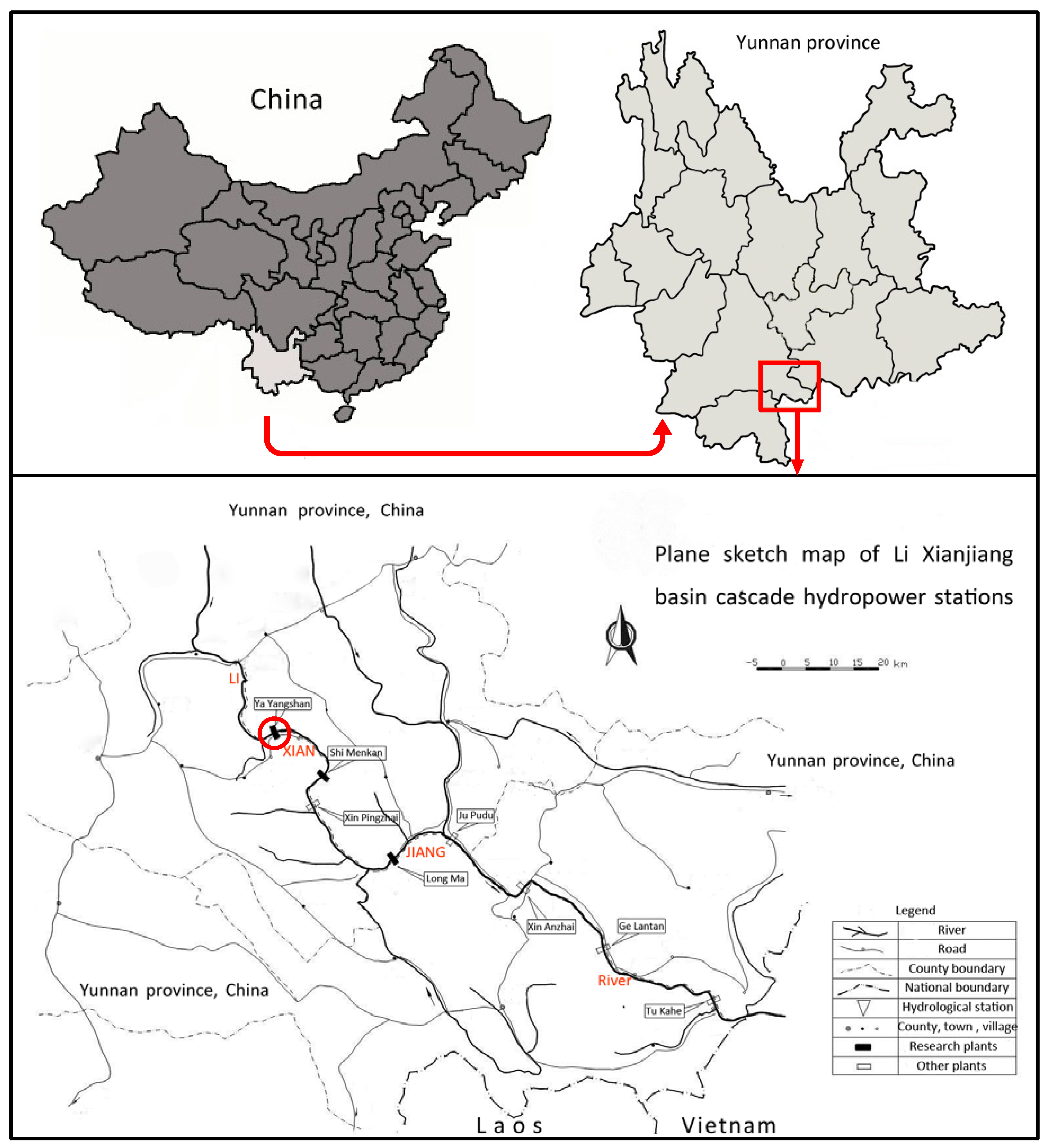
3.1. Data and Brief Introduction to Research Object

Li Xianjiang River is a tributary of Red River, and it is located in Yunnan province of China. There is a 473 km main channel, 1790 m natural drop, and 19,309 km² control area in China. At the border of China, the annual average runoff is 460 m³/s. There are eight hydropower stations on the main channel, i.e., Tu Kahe, Ge Lantan, Xin Anzhai, Ju Pudu, Long Ma, Xin Pingzhai, Shi Menkan, and Ya Yangshan from downstream to upstream. Three hydropower stations in these hydropower stations have the seasonal regulation performance, which are Long Ma, Shi Menkan, and Ya Yangshan. The Ya Yangshan is the topmost and the dominant hydropower station of the main channel, whose operation level can determine the whole power generation benefit of the cascade reservoirs. Therefore, Ya Yangshan hydropower station is selected as the research object in this paper. Location of the selected hydropower station in Li Xianjiang River basin is shown in Figure 7 [40], and its basic parameters are shown in

Table 2. Parameters of Ya Yangshan hydropower station

Items	Unit	Value	Items	Unit	Value
Normal level	m	835	Annual power generation	GWh	496.0
Dead level	m	818	Coefficient of head loss	10−5	8.658
Total volume	Gm3	0.308	Biggest head loss	m	5.590
Regulation volume	Gm3	0.134	Coefficient of output	None	8.3
Regulation performance	None	Season	Flood control level	m	818
Design assurance rate	%	95	Flood season	None	6~10
Guaranteed output	MW	23.2	--	--	--

. The available long series of runoff data for this hydropower station is from 1957 to 2000, a total of 43 years.

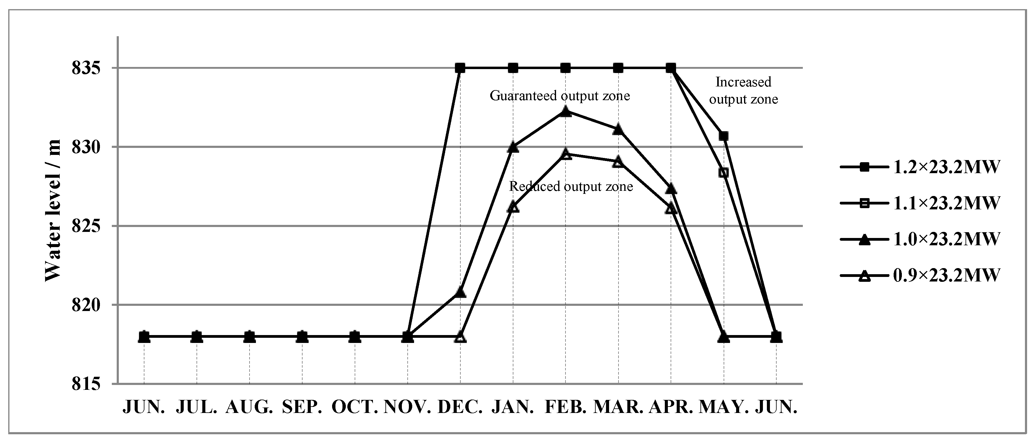
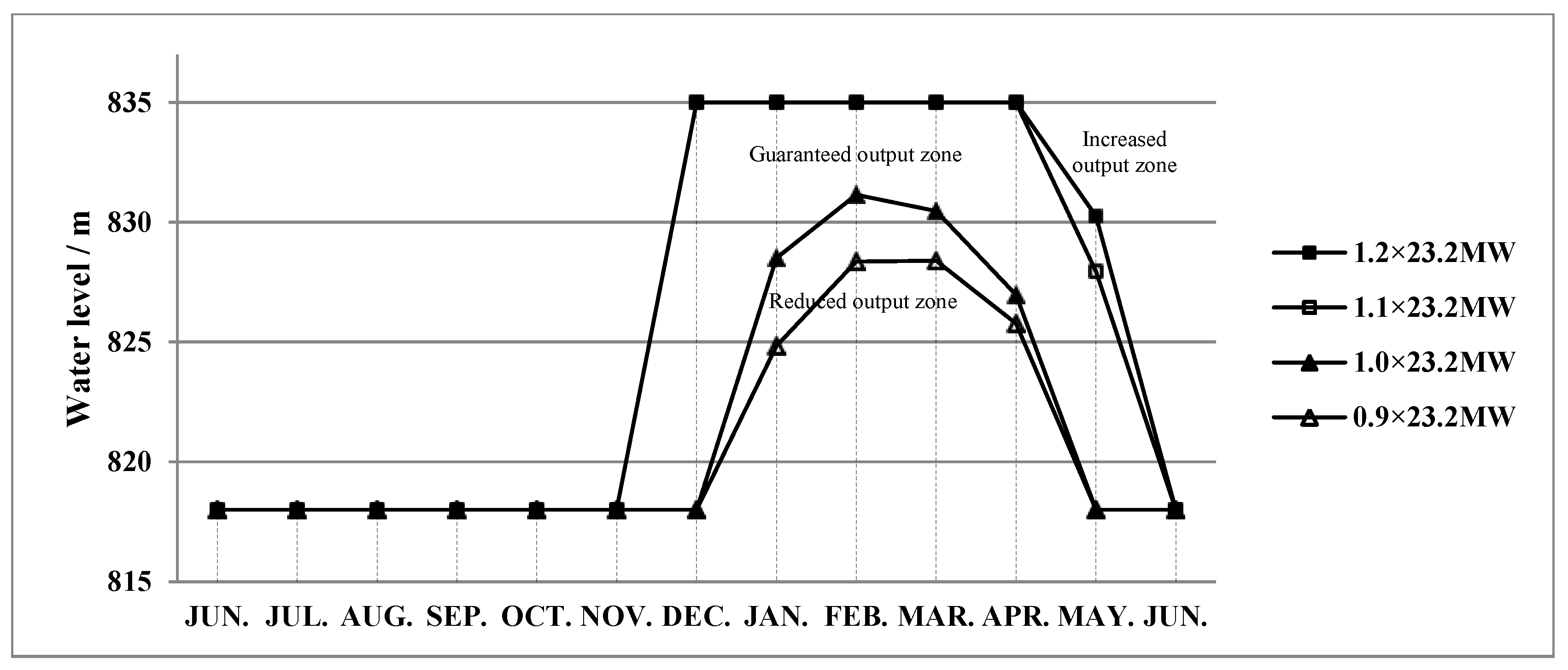
3.2. Results of the Two Methods

As can be seen from Table 2, the guaranteed output of Ya Yangsha reservoir is 23.2 MW, and the assurance rate is 95%. However, in the actual calculation by conventional method [41] or DP based optimization method (as shown in Figure 5), it was found that the requirements of the guaranteed output and assurance rate cannot be satisfied at the same time. As we know, the assurance rate and power generation of a hydropower station are usually gradually reduced with the increase of the guaranteed output, so it is an effective way to reduce the guaranteed output to improve the assurance rate and power generation. There is an inverse relationship between the assurance rate and guaranteed output in the hydropower station operation. Therefore, for facilitating the comparative analysis, this paper firstly provides the results of the conventional method, in which only one indicator (the guaranteed output or assurance rate) is satisfied. Then, the results of DP based method will be provided in the same form.

For the conventional method, when the guaranteed output of the reservoir is 23.2 MW, the simulation results of the conventional reservoir operation chart through a long series of historical runoff can be obtained. The assurance rate is 93% and the power generation is 496.3 GWh. The corresponding reservoir operation chart is shown in Figure 8. Where, the 1.0 × 23.2 MW corresponds to the basic operation curve, the 1.1 × 23.2 MW corresponds to the increased output curve whose output is 1.1 times the guaranteed output, the 1.2 × 23.2 MW corresponds to the increased output curve whose output is 1.2 times the guaranteed output, and the 0.9 × 23.2 MW corresponds to the reduced output curve whose output is 0.9 times the guaranteed output.

When the assurance rate of the reservoir is asked to not less than 95% in the conventional method, the simulation results of the conventional method show that, the guaranteed output is 22.4 MW, and power generation is 496.7 GWh. The corresponding reservoir operation chart is shown in Figure 9.

For the DP based method, when the guaranteed output of the reservoir is 23.2 MW, the reservoir operation chart obtained by the proposed method in this paper is shown in Figure 10. Its simulation results through a long series of historical runoff show that, the corresponding assurance rate is 94%, and the power generation is 498.9 GWh.

When the assurance rate of the reservoir is asked to not less than 95% in the DP based method, the reservoir operation chart obtained by the proposed method is shown in Figure 11. Its simulation results show that the corresponding guaranteed output is 23.0 MW, and the power generation is 501.2 GWh.

Whether the actual dispatcher takes the assurance rate or the guaranteed output as the main control factor to decide the final reservoir operation chart, the actual operation requirements and situations of hydropower station are needed. For the hydropower station operation in Li Xianjiang River, considering the demands of power grid security and stability, there is more focus on the reliability of hydropower generation. Thus, this paper takes the assurance rate as the main control factor to determine the final reservoir operation chart. In view of this, the second case mentioned above conforms more to the actual situation.

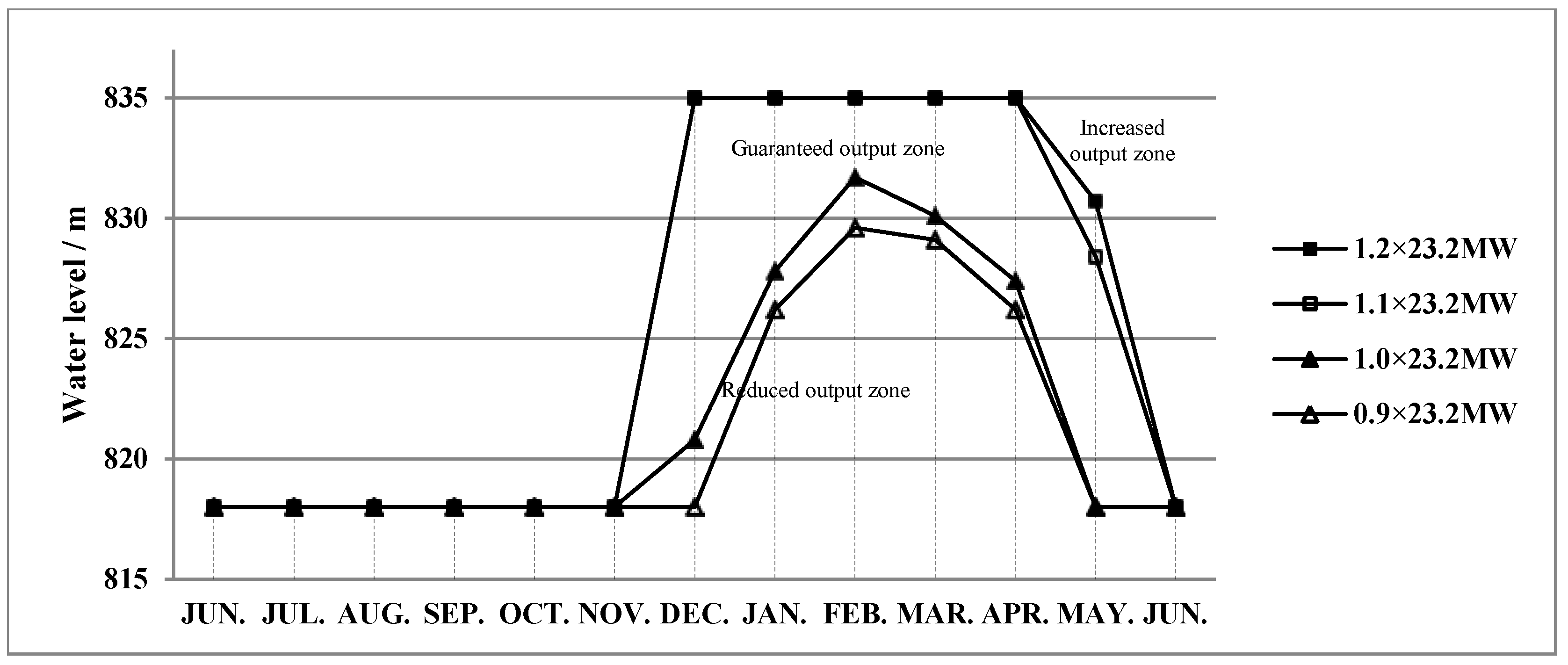
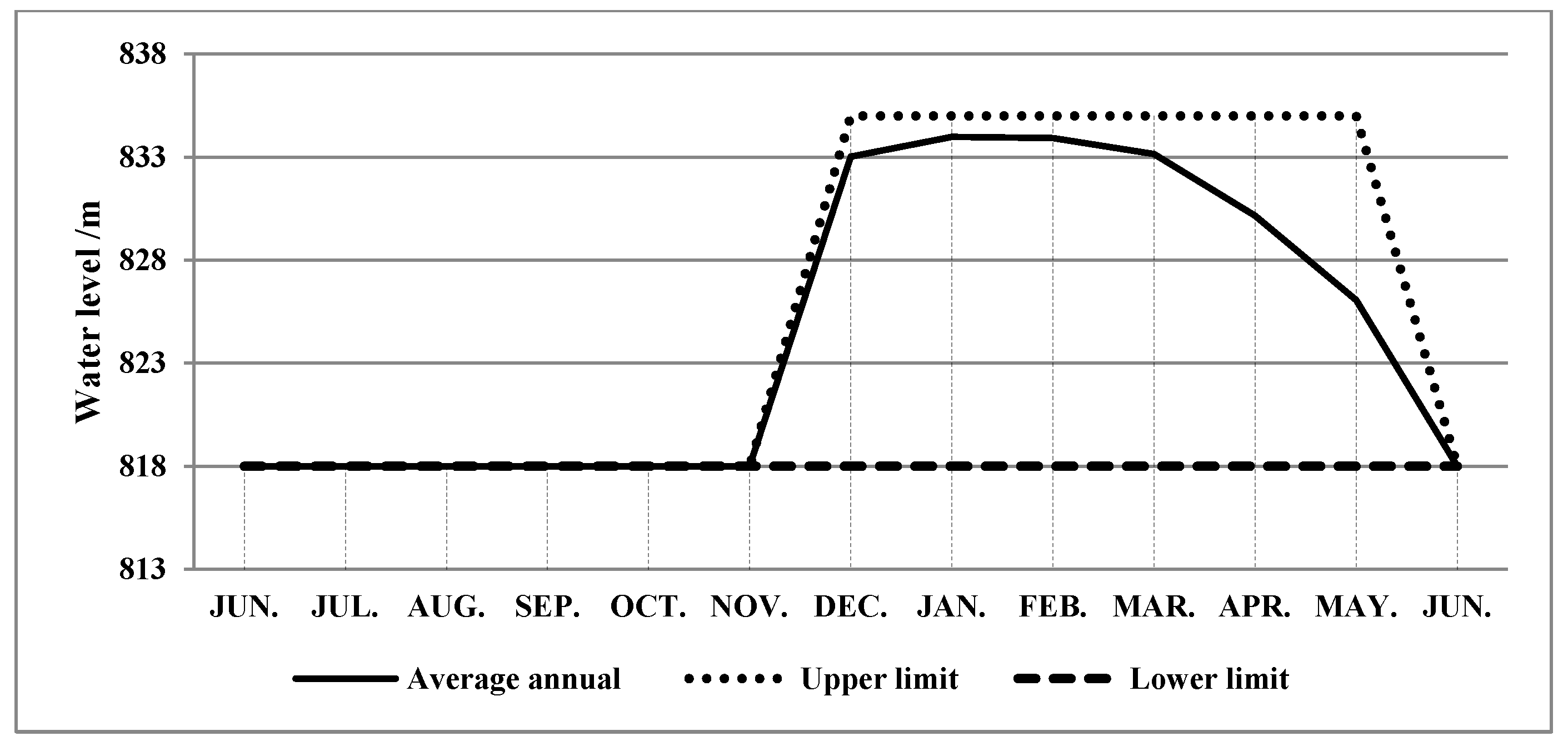
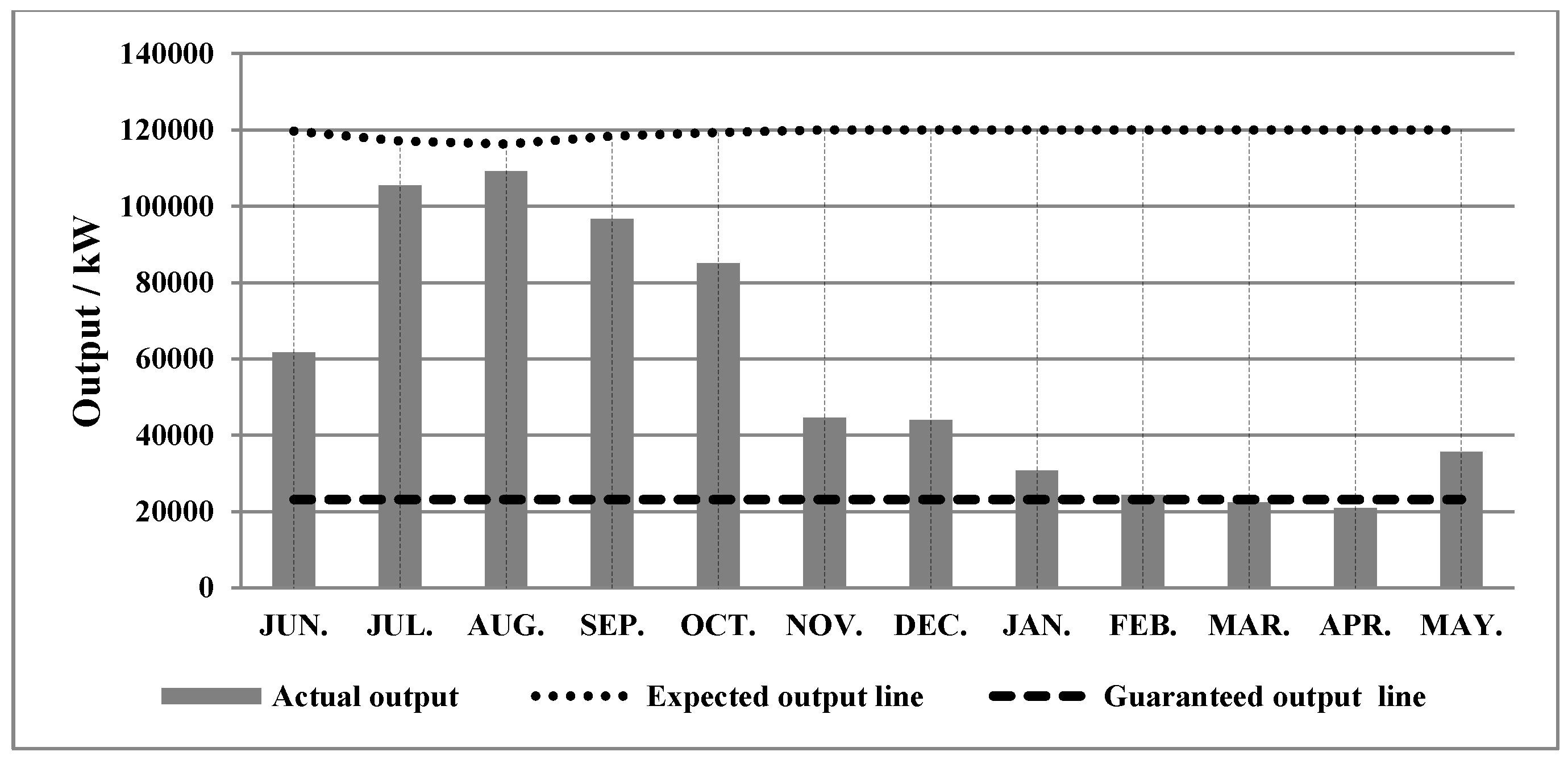
3.3. Contrastive Analysis

In order to facilitate the comparative analysis, the results of the two methods under the same boundary conditions are put together. For example, when the guaranteed output of the conventional method and the proposed method are both the same 23.2 MW, the simulation results of each method are shown in

Table 3. Simulation results of the two methods when the guaranteed outputs are both 23.2 MW.

Item	Unit	Conventional Method	Proposed Method	Incremental	Growth
Assurance rate	--	93%	94%	1%	1.08%
Annual power generation	GWh	496.3	498.9	2.6	0.52%

. When the assurance rate of the two methods are both asked to not less than 95%, the simulation results of each method are shown in

Table 4. Simulation results of the two methods when the assurance rates are both 95%.

Item	Unit	Conventional Method	Proposed Method	Incremental	Growth
Guaranteed output	MW	22.4	23.0	0.6	2.68%
Annual power generation	GWh	496.7	501.2	4.5	0.91%

.

From Table 3, it can be seen that, compared with the conventional method, the assurance rate and power generation of the proposed method in this paper both have a certain degree of improvement when the guaranteed output of the two methods are the same 23.2 MW, and the growth is 0.52% and 1.08%, respectively. From Table 4, it can be seen that, when the assurance rate of the two methods are both asked to not less than 95%, the power generation and guaranteed output of the proposed method also have a certain degree of improvement compared with the conventional method, and the growth is 0.91% and 2.68%, respectively. So, from the aspects of assurance rate, guaranteed output, and power generation, all the simulation results indicate that the proposed method based on DP in this paper is better than the conventional method.

Besides, in comparing the two situations—i.e., the situation of the guaranteed output of the two methods are the same 23.2 MW and the situation of the assurance rate of the two methods are both asked to not less than 95%—it is found that the latter situation has a better result on the annual power generation, that is, 0.91% growth is greater than 0.52% growth. This result is consistent with that this paper takes the assurance rate as the main control factor to determine the final reservoir operation chart.

Compared the Figure 10 with Figure 8, it can be found that the guaranteed output zone of the Figure 10 has relatively expanded a little, and the reduced output zone has narrowed down. This change brings in a corresponding improvement for the assurance rate, which is consistent with the simulation results in Table 3 (increased from 93% to 94%).

Compared the Figure 11 with Figure 9, it can be seen that the guaranteed output zone of the Figure 11 has relatively expanded, and the reduced output zone has narrowed down. Generally, this change will make the assurance rate increase if the guaranteed output unchanged. However, the guaranteed output increased, which is changed to 23.0 MW from 22.4 MW at this moment, so the assurance rate remains unchanged.

Similarly, compared the Figure 11 with Figure 10, it can be found that the guaranteed output zone of the Figure 11 has relatively expanded, and the reduced output zone has narrowed down, which will make the assurance rate increase if the guaranteed output fixed. However, at this moment, the change of the operation zones cannot make the assurance rate reach 95%, therefore, the guaranteed output needs to be reduced (changed from 23.2 to 23.0), so that to make the assurance rate reach 95%.

In addition, in order to compare the results with that of deterministic DP, this paper implements the direct optimization by DP when the assurance rate is asked to not less than 94% and 95% respectively, and the guaranteed output is fixed as 23.2 MW and 23.0 MW correspondingly. The optimization results are as follows. When the assurance rate is 94% and the guaranteed output is 23.2 MW, the annual average power generation of DP is 500.7 GWh, and when the assurance rate is 95% and the guaranteed output is 23.0 MW, it is 502.8 GWh.

For the proposed method in this paper, the power generation is 498.9 GWh when the assurance rate is 94% (as shown in Table 3), and the power generation is 501.2 GWh when the assurance rate is 95% (as shown in Table 4), which are both slightly less than the results of DP. However, the difference is small, which is only 1.8 GWh (0.36%) and 1.6 GWh (0.32%), respectively. This result indicates that the proposed method in this paper has maintained the global convergence of DP well to a certain extent.

Taking the proposed method as an example, the average annual water level variation of Ya Yangshan reservoir is shown in Figure 12 when the assurance rate is 95%, and the average annual output variation is shown in Figure 13.

From Figure 12, it can be seen that the reservoir filling up quickly at the beginning stages of the storage period, and then maintains the operation with a relatively high water level, so that to increase the water head efficiency. In the supply period, the reservoir’s water level drops homogeneous, which makes the output uniformed, so that to avoid the concentrated destruction of output or water abandonment at the last few stages of the entire planning horizon. Correspondingly, from Figure 13, it can be seen that the reservoir basically maintains the guaranteed output in the supply period, except for the increased output of the last stage because of emptying the reservoir. Thus, it can be concluded that the average annual operation process is conformed to the actual operation principle, which reflects the consistency of actual facts with the simulation results of the obtained reservoir operation chart. Hence, the rationality of the proposed method in this paper is further proved.

4. Summary and Conclusions

Reservoir operation chart plays a very important role in the actual operation of reservoir, and this paper presents a new method to calculate the reservoir operation chart based on DP. Compared with the conventional drawing method, it is more direct and effective to calculate the optimal operation chart through the DP model directly, and to a certain extent, it can guarantee the global convergence of the results because of the global convergence of DP. This paper took the Ya Yangshan reservoir of Li Xianjiang River in southwest China as an example to derive the operation chart by the proposed method, and the following conclusions can be summarized:

(1) Through the simulation of case study, the results show that the proposed method presents better performance compared with the conventional method, 2.68% growth on assurance rate and 0.91% growth on power generation can be obtained by the proposed method. Besides, the simulation operation processes (water level and output) of the proposed method are conformed to the actual operation principle, this reflects the consistency of actual facts with the simulation results of the obtained reservoir operation chart. So, the validity and rationality of the proposed method are verified by the simulation results.

(2) Compared with the direct optimization results of DP, although the power generations of the proposed method under two assurance rates are both slightly less than that of DP, the differences are small, which is only 0.36% and 0.32% decline, respectively. This result shows that the proposed method in this paper has maintained the global convergence of DP to a certain extent.

(3) However, the advantage of the proposed method is not very significant compare to the conventional method, and the increase on power generation is only 0.91%. The possible reason may be the simplified treatments in the reverse recursion procedure, which cannot give full play to the global convergence of DP.

In summary, the study in this paper has achieved some good results. The proposed method can avoid the shortage of other methods in drawing and optimizing the reservoir operation chart, and make up for the deficiency of the research on DP based reservoir operation chart optimization. However, some work still needs to be done in the future. For improving the significance of this method, fine processing is needed in the reverse recursion procedure, and for the validity of the proposed method for other hydropower stations, more case studies need to be done, especially the joint operation chart derivation of cascade reservoirs. In addition, in the derivation of joint operation chart of cascade reservoirs by DP, there may be a long computing time, so the parallel computing techniques or other measures need to be adopted.

References

1. Yüksel, I. Hydropower for sustainable water and energy development. Renew. Sustain. Energy Rev. 2010, 14, 462–469. [Google Scholar] [CrossRef]
2. Bozorg-Haddad, O.; Garousi-Nejad, I.; Loáiciga, H.A. Extended multi-objective firefly algorithm for hydropower energy generation. J. Hydroinform. 2017, 19, 734–751. [Google Scholar] [CrossRef]
3. Spaenhoff, B. Current status and future prospects of hydropower in Saxony (Germany) compared to trends in Germany, the European Union and the World. Renew. Sustain. Energy Rev. 2014, 30, 518–525. [Google Scholar] [CrossRef]
4. Li, F.F.; Qiu, J. Multi-objective optimization for integrated hydro-photovoltaic power system. Appl.Energy 2016, 167, 377–384. [Google Scholar] [CrossRef]
5. Gebretsadik, Y.; Fant, C.; Strzepek, K.; Arndt, C. Optimized reservoir operation model of regional wind and hydro power integration case study: Zambezi basin and South Africa. Appl. Energy 2016, 161, 574–582. [Google Scholar] [CrossRef]
6. Sharma, V.; Jha, R.; Naresh, R. Optimal multi-reservoir network control by two phase neural network. Elec. Power Syst. Res. 2004, 68, 221–228. [Google Scholar] [CrossRef]
7. Paish, O. Micro-hydropower: Status and prospects. Proc. Inst. Mech. Eng. Part A J. Power Energy 2005, 216, 31–40. [Google Scholar] [CrossRef]
8. Pérez-Sánchez, M.; Sánchez-Romero, F.J.; Ramos, H.M.; López-Jiménez, P.A. Energy Recovery in Existing Water Networks: Towards Greater Sustainability. Water 2017, 2, 97. [Google Scholar] [CrossRef]
9. George, C.B. Feasibility study of a hybrid wind/hydropower-system for low-cost electricity production. Appl. Energy 2002, 72, 599–608. [Google Scholar]
10. Zhang, Y.K.; Jiang, Z.Q.; Ji, C.M.; Sun, P. Contrastive analysis of three parallel modes in multi-dimensional dynamic programming and its application in cascade reservoirs operation. J. Hydrol. 2015, 529, 22–34. [Google Scholar] [CrossRef]
11. Lu, D.; Wang, B.D.; Wang, Y.D.; Zhou, H.C.; Liang, Q.H.; Peng, Y.; Roskilly, T. Optimal operation of cascade hydropower stations using hydrogen as storage medium. Appl. Energy 2015, 137, 56–63. [Google Scholar] [CrossRef]
12. Consoli, S.; Matarazzo, B.; Pappalardo, N. Operating rules of an irrigation purposes reservoir using multi-objective optimization. Water Resour. Manag. 2008, 22, 551–564. [Google Scholar] [CrossRef]
13. de Araújo, J.C.; Mamede, G.L.; de Lima, B.P. Hydrological Guidelines for Reservoir Operation to Enhance Water Governance: Application to the Brazilian Semiarid Region. Water 2018, 10, 1628. [Google Scholar] [CrossRef]
14. Lund, J.R.; Guzman, J. Derived operating rules for reservoirs in series or in parallel. J. Water Resour. Plan. Manag. 1999, 125, 143–153. [Google Scholar] [CrossRef]
15. Catalão, J.P.S.; Pousinho, H.M.I.; Contreras, J. Optimal hydro scheduling and offering strategies considering price uncertainty and risk management. Energy 2012, 37, 237–244. [Google Scholar] [CrossRef]
16. Wu, C.L.; Chau, K.W.; Li, Y.S. Predicting monthly stream flow using data-driven models coupled with data-preprocessing techniques. Water Resour. Res. 2009, 45, 1–23. [Google Scholar] [CrossRef]
17. Ma, C.; Lian, J.J.; Wang, J.N. Short-term optimal operation of Three-gorge and Gezhouba cascade hydropower stations in non-flood season with operation rules from data mining. Energy Convers. Manag. 2013, 65, 616–627. [Google Scholar] [CrossRef]
18. Ji, C.M.; Zhou, T.; Huang, H.T. Operating Rules Derivation of Jinsha Reservoirs System with Parameter Calibrated Support Vector Regression. Water Resour. Manag. 2014, 28, 2435–2451. [Google Scholar] [CrossRef]
19. Shao, L.; Wang, L.P.; Huang, H.T.; Yang, Z.J.; Yu, S. Optimization of the reservoir operation chart of hydropower station and its application-based on hybrid genetic algorithm and simulated annealing. Power Syst. Prot. Control 2010, 38, 40–43. [Google Scholar]
20. Yu, S.; Ji, C.M.; Xie, W.; Liu, F. Instructional Mutation Ant Colony Algorithm in Application of Reservoir Operation Chart Optimization. In Proceedings of the Fourth International Symposium on Knowledge Acquisition and Modeling, Sanya, China, 8–9 October 2011; pp. 462–465. [Google Scholar]
21. Cheng, C.T.; Yang, F.Y.; Wu, X.Y.; Su, H.Y. Link the simulation with dynamic programming successive approximations to the study on optimal operation chart of cascade reservoirs. J. Hydroelectr. Eng. 2010, 29, 71–77. [Google Scholar]
22. Guo, Z.Z.; Wu, J.K.; Kong, F.N.; Zhu, Y.N. Long-term Optimization Scheduling Based on Maximal Storage Energy Exploitation of Cascaded Hydro-plant Reservoirs. Proc. CSEE 2010, 30, 20–25. [Google Scholar]
23. Huang, J.W.; Hu, Y.; Li, H.S. Model of Joint Optimizing Operation for Cascade Reservoirs and Application. China Water Power Electrif. 2011, 12, 11–15. [Google Scholar]
24. Baskar, S.; Subbaraj, P.; Rao, M.V.C. Hybrid real coded genetic algorithm solution to economic dispatch problem. Comput. Electr. Eng. 2003, 29, 407–419. [Google Scholar] [CrossRef]
25. Momtahen, S.h.; Dariane, A.B. Direct search approaches using genetic algorithms for optimization of water reservoir operating policies. J. Water Resour. Plan. Manag. 2007, 133, 202–209. [Google Scholar] [CrossRef]
26. Cai, X.; McKinney, D.C.; Lasdon, L.S. Solving nonlinear water management models using a combined genetic algorithm and linear programming approach. Adv. Water Resour. 2001, 24, 667–676. [Google Scholar] [CrossRef]
27. Zhang, R.; Zhou, J.; Zhang, H.; Liao, X.; Wang, X. Optimal Operation of Large-Scale Cascaded Hydropower Systems in the Upper Reaches of the Yangtze River, China. J. Water Resour. Plan. Manag. 2014, 140, 480–495. [Google Scholar] [CrossRef]
28. Cheng, C.T.; Shen, J.J.; Wu, X.Y. Short-Term Hydro scheduling with Discrepant Objectives Using Multi-Step Progressive Optimality Algorithm. J. Am. Water Resour. Assoc. 2012, 48, 464–479. [Google Scholar] [CrossRef]
29. Lu, B.; Li, K.; Zhang, H.; Wang, W.; Gu, H. Study on the optimal hydropower generation of Zhelin reservoir. J. Hydro-Environ. Res. 2013, 7, 270–278. [Google Scholar] [CrossRef]
30. Jiang, Z.; Ji, C.; Qin, H.; Feng, Z. Multi-stage progressive optimality algorithm and its application in energy storage operation chart optimization of cascade reservoirs. Energy 2018, 148, 309–323. [Google Scholar] [CrossRef]
31. Jiang, Z.; Qin, H.; Ji, C.; Feng, Z.; Zhou, J. Two Dimension Reduction Methods for Multi-Dimensional Dynamic Programming and Its Application in Cascade Reservoirs Operation Optimization. Water 2017, 9, 634. [Google Scholar] [CrossRef]
32. Vincenzo, M.; Gianfranco, R.; Francesco, A.T. Application of dynamic programming to the optimal management of a hybrid power plant with wind turbines, photovoltaic panels and compressed air energy storage. Appl. Energy 2012, 97, 849–859. [Google Scholar]
33. Jiang, Z.; Qin, H.; Wu, W.; Qiao, Y. Studying Operation Rules of Cascade Reservoirs Based on Multi-Dimensional Dynamics Programming. Water 2017, 10, 20. [Google Scholar] [CrossRef]
34. Zhao, T.; Zhao, J. Improved multiple-objective dynamic programming model for reservoir operation optimization. J. Hydroinform. 2014, 16, 1142–1157. [Google Scholar] [CrossRef]
35. Sordo-Ward, A.; Gabriel-Martin, I.; Bianucci, P.; Garrote, L.A. Parametric Flood Control Method for Dams with Gate-Controlled Spillways. Water 2017, 9, 237. [Google Scholar] [CrossRef]
36. Jiang, Z.; Wu, W.; Qin, H.; Zhou, J. Credibility theory based panoramic fuzzy risk analysis of hydropower station operation near the boundary. J. Hydrol. 2018, 565, 474–488. [Google Scholar] [CrossRef]
37. Jiang, Z.; Li, R.; Li, A.; Ji, C. Runoff forecast uncertainty considered load adjustment model of cascade hydropower stations and its application. Energy 2018, 158, 693–708. [Google Scholar] [CrossRef]
38. Kuriqi, A.; Ardiçlioǧlu, M. Investigation of hydraulic regime at middle part of the Loire River in context of floods and low flow events. Pollack Period. 2018, 13, 145–156. [Google Scholar] [CrossRef]
39. Selenica, A.; Kuriqi, A.; Ardicioglu, M. Risk assessment from floodings in the rivers of Albania. In Proceedings of the International Balkans Conference on Challenges of Civil Engineering, Tirana, Albania, 19–21 May 2011. [Google Scholar]
40. Ji, C.M.; Jiang, Z.Q.; Sun, P.; Zhang, Y.K.; Wang, L.P. Research of multi-dimensional dynamic programming based on multi-layer nested structure and its application in cascade reservoirs. J. Water Resour. Plan. Manag. 2015, 141, 1–13. [Google Scholar] [CrossRef]
41. Jiang, Z.; Li, A.; Ji, C.; Qin, H.; Yu, S.; Li, Y. Research and application of key technologies in drawing energy storage operation chart by discriminant coefficient method. Energy 2016, 114, 774–786. [Google Scholar] [CrossRef]
Figure 1. Schematic diagram of conventional operation chart.
Energies 11 03355 g001
Figure 2. Feasible water level range of each operation curve after discretization.
Energies 11 03355 g002
Figure 3. Schematic diagram of the stage-operation-chart.
Energies 11 03355 g003
Figure 4. The possible space of discretized water level combinations.
Energies 11 03355 g004
Figure 5. Flowchart of calculating the reservoir operation chart based on DP.
Energies 11 03355 g005
Figure 6. Schematic diagram of deriving the beginning water level by the assumption calculation.
Energies 11 03355 g006
Figure 7. The location of Ya Yangshan hydropower station in Li Xianjiang River basin.
Energies 11 03355 g007
Figure 8. Conventional reservoir operation chart considering the guaranteed output constraint.
Energies 11 03355 g008
Figure 9. Conventional reservoir operation chart considering the assurance rate constraint.
Energies 11 03355 g009
Figure 10. DP based reservoir operation chart considering the guaranteed output constraint.
Energies 11 03355 g010
Figure 11. DP based reservoir operation chart considering the assurance rate constraint.
Energies 11 03355 g011
Figure 12. Average annual water level variation of Ya Yangshan reservoir.
Energies 11 03355 g012
Figure 13. Average annual output variation of Ya Yangshan reservoir.
Energies 11 03355 g013