Multiobjective Joint Economic Dispatching of a Microgrid with Multiple Distributed Generation


Abstract
:1. Introduction
2. Joint Economic Dispatch Strategy for MGs and the Main Grid
2.1. The MG System Model with Multiple DGs
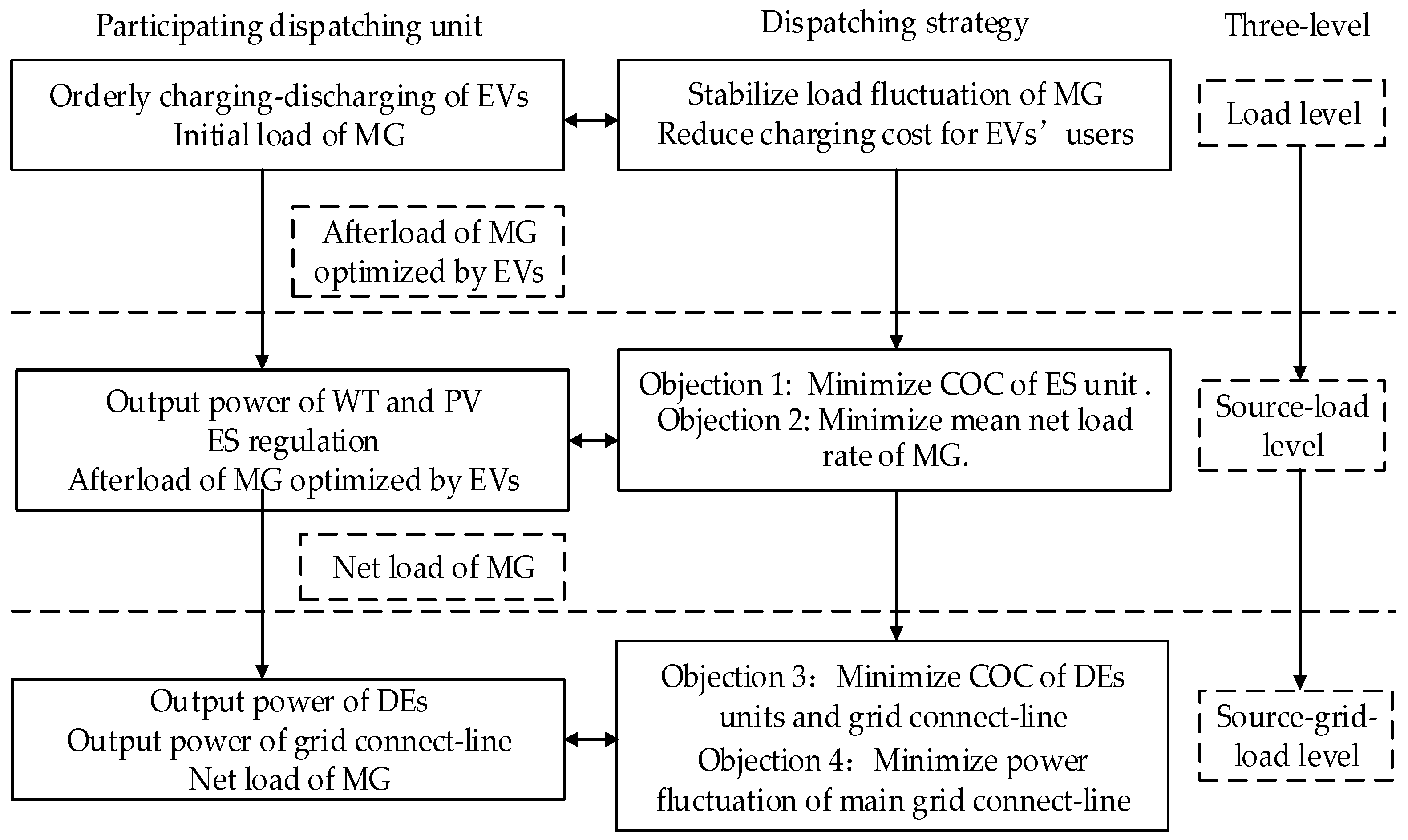
2.2. Strategy Overview
2.3. Dispatch Strategy for the Load Level
2.4. Dispatch Strategy for the Source-Load Level
- The SOC of ES unit constraint:
- Upper and lower output limit of ES power output:where and are, respectively, the maximum and minimum power output of the ES unit.
2.5. Dispatch Strategy for the Source-Grid-Load Level
- Upper and lower limit constraints of DE power output:
- Climbing power limit of DE:
- Upper and lower output limits of the main grid side:
- Power balance equation:where and are, respectively, the maximum and minimum power output of a DE unit; and are the maximum and minimum climbing power of a DE unit; and and are, respectively, the maximum and minimum power output of the connect line of the main grid.
2.6. Dispatch Strategy for the Source-Grid-Load Level Under Isolated Grid
3. Solution Method and Simulation Parameters
3.1. Solution Method
- Initializing the particle swarm. is the population size, is the particle dimension, and is the number of population evolution iterations; the position and velocity of each particle (, ) are randomly initialized.
- Calculating the fitness values of particles.
- Calculating the particle’s individual optimum and global historical optimum .
- Selecting the new optimal value by comparing the function values of the maximum or minimum fitness functions.
- Updating the particle velocity and position according to the following Equation (20) and Equation (21), respectively. If a dimension of the particle exceeds the boundary, the dimension data are re-initialized.In the equations above, is inertia weight; is the number of iterations; and are nonnegative constants, called acceleration factors; and are random numbers distributed in the [0,1] interval; is the individual optimum value of the dimension at iteration ; and is the global historical optimum value of the dimension at iteration , .
- Screening the noninferior solutions in the current particle swarm, adding the elite set, and eliminating the inferior solutions in the elite set.
- If the termination condition is satisfied, the loop is completed; otherwise, we return to Step 2.
3.2. Simulation Parameters
4. Results and Analysis
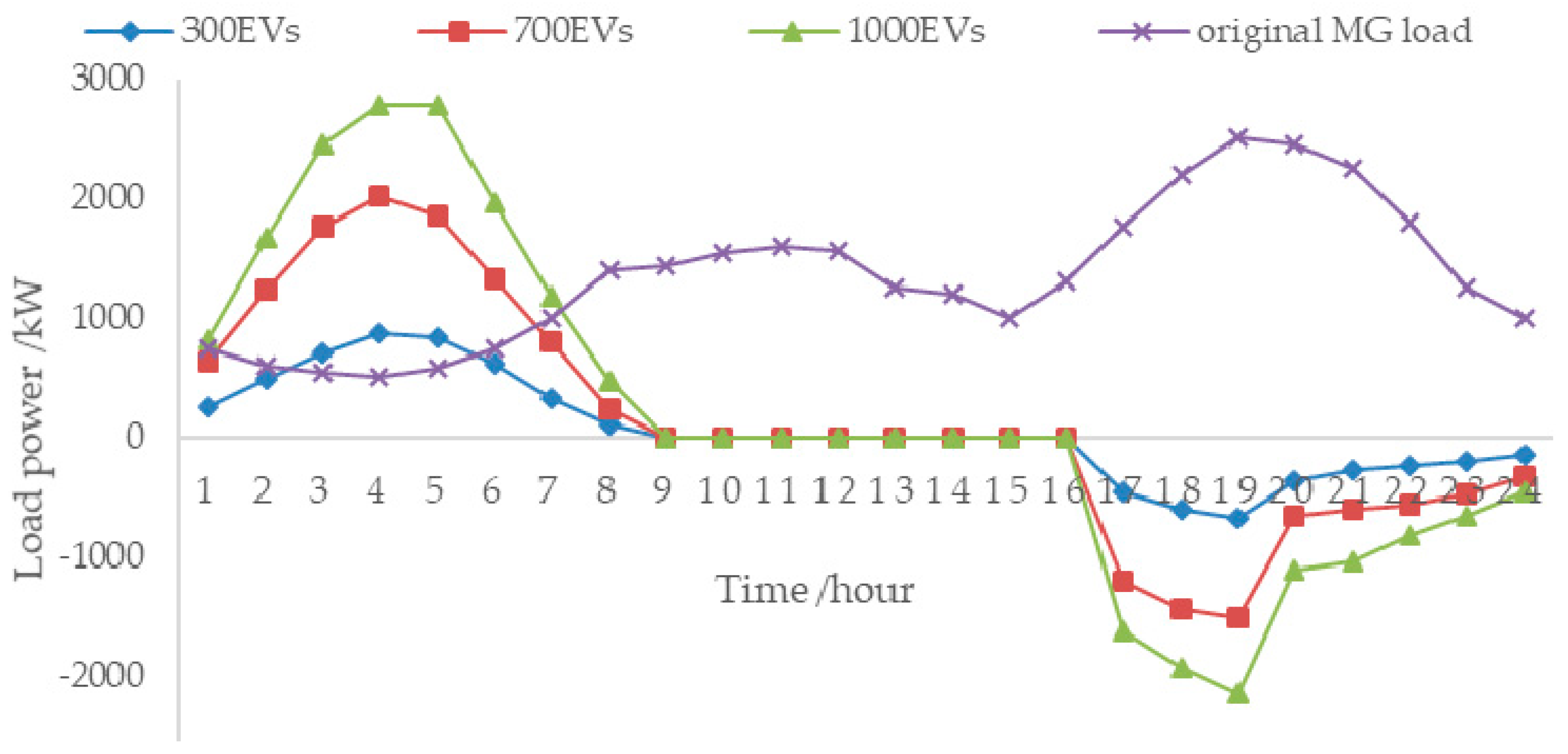
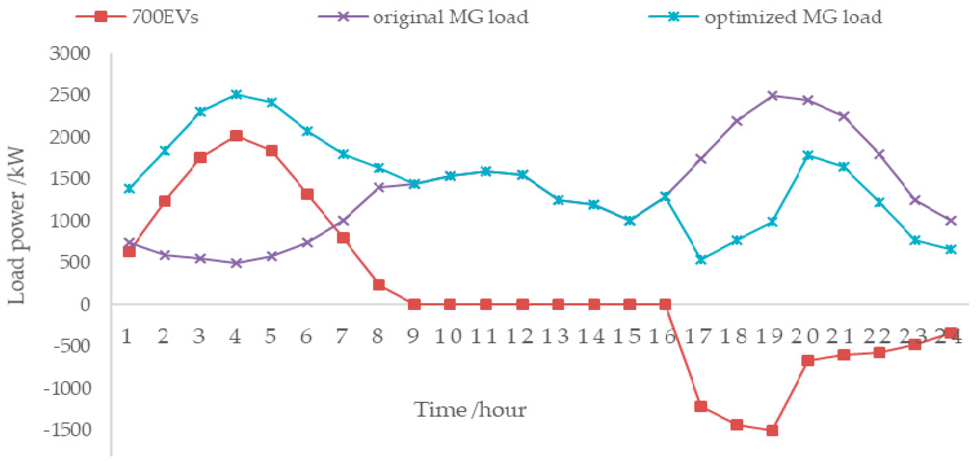
4.1. Results and Analysis of Load Level Optimization
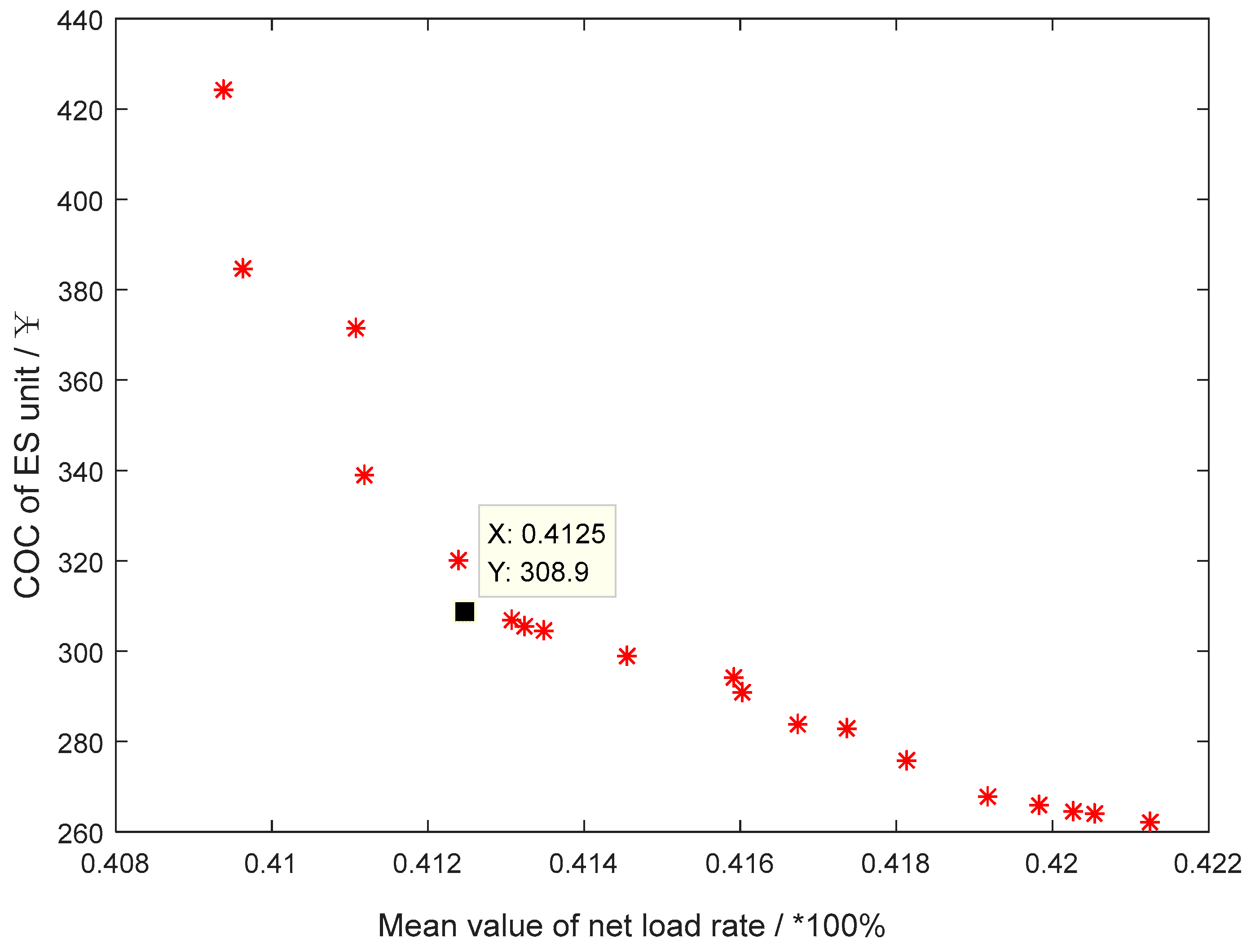
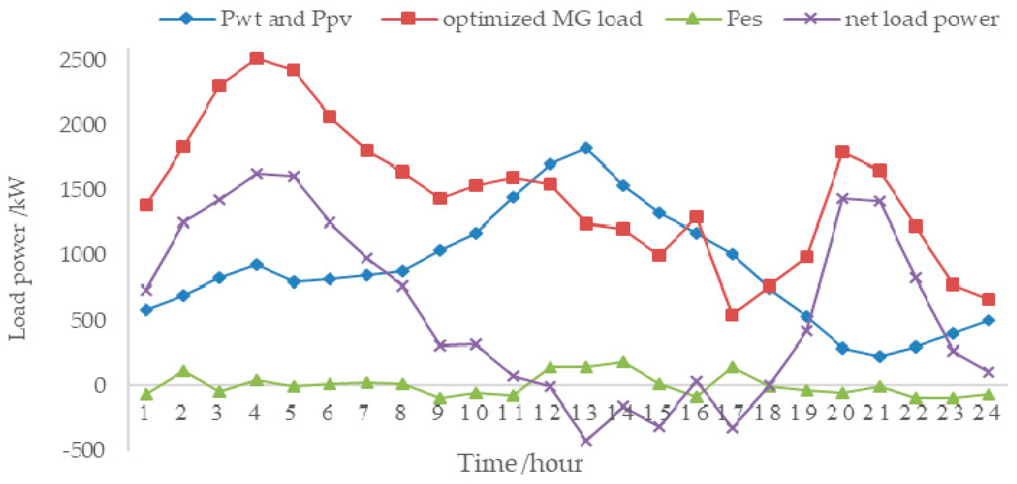
4.2. Results and Analysis of Source-Load Level Optimization
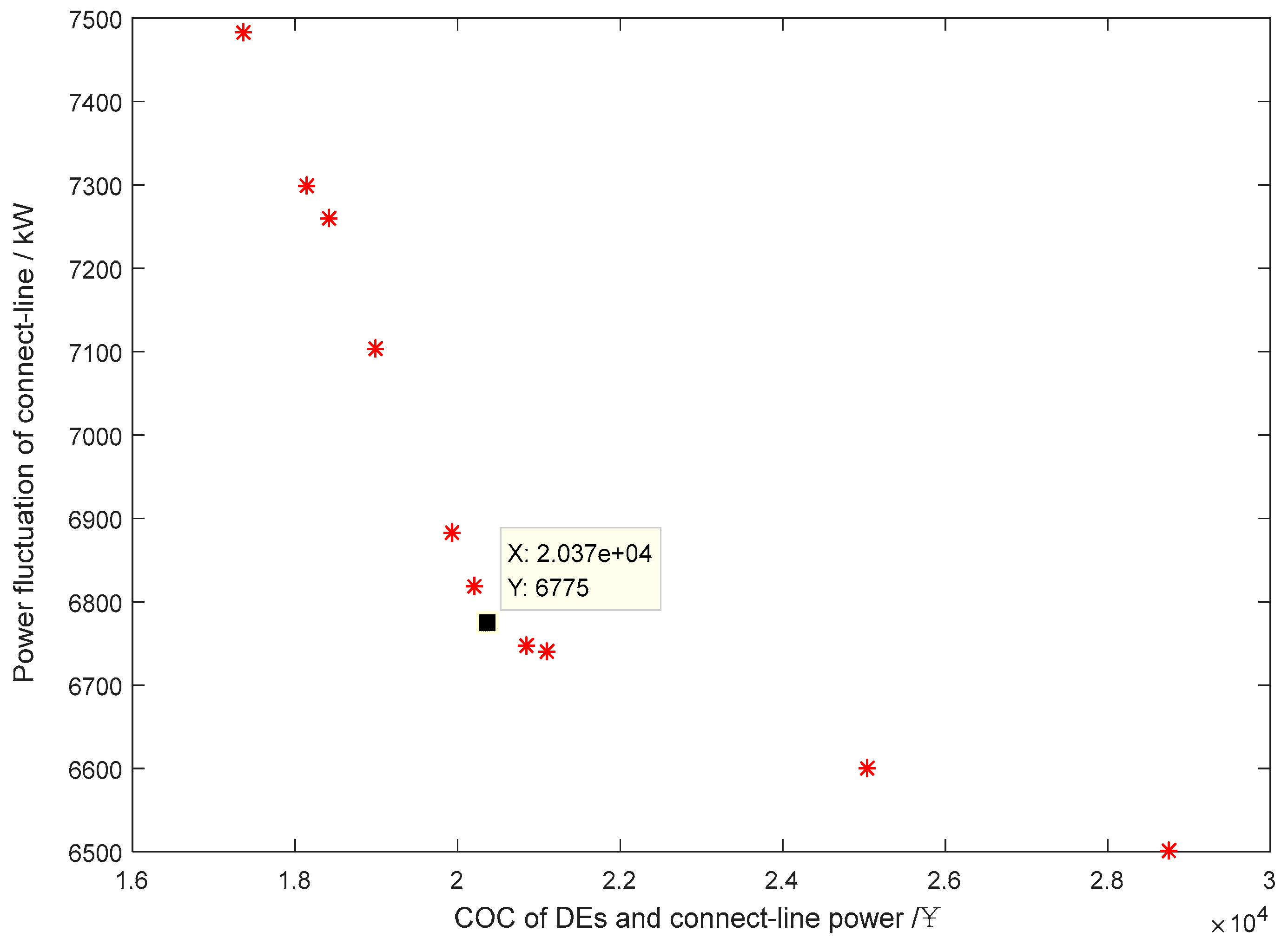
4.3. Results and Analysis of Source-Grid-Load Level Optimization
4.4. Comparison and Analysis
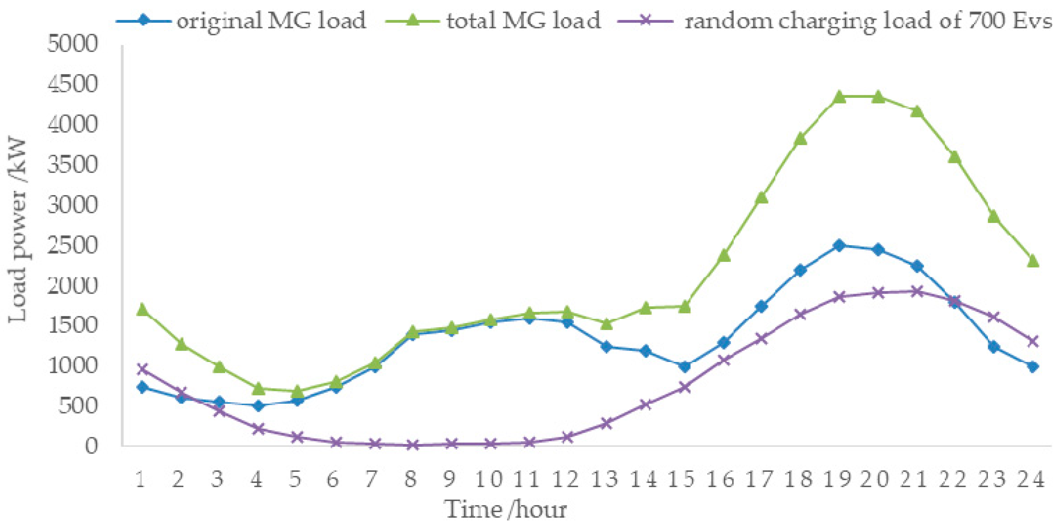
4.4.1. Analysis of the Results of the Economic Dispatching Operation of a Multiobjective Hierarchical MG with Random Charging of EVs
4.4.2. Analysis of the Results of the Economic Dispatching Operation of a Multiobjective Hierarchical MG under Isolated Grid Operation
5. Conclusions
Author Contributions
Funding
Conflicts of Interest
Nomenclature
| Abbreviations | |
| MG | Microgrid |
| COC | comprehensive operating cost |
| ES | energy storage |
| EV | electric vehicle |
| TOU | time of use |
| DE | diesel engine |
| DG | distributed generation |
| CHP | Combined Heat and Power |
| WT | wind turbines |
| PV | photovoltaics |
| SOC | state of charge |
| MPSO | Multiobjective Particle Swarm Optimization |
| Symbols | |
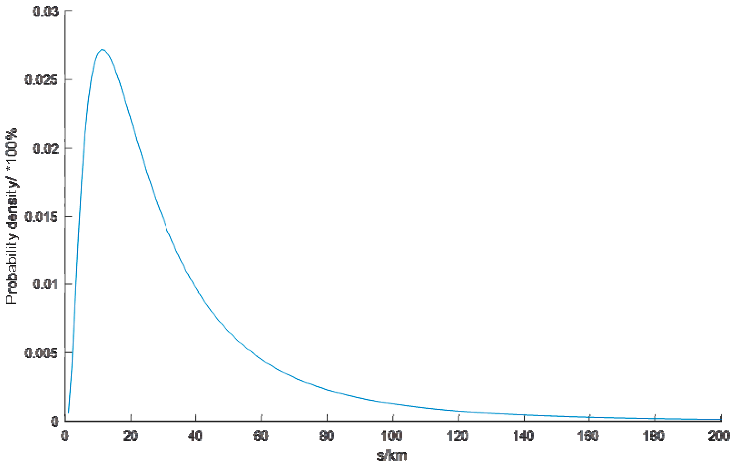
| daily travel distance of EV | |
| expectation of EV’s daily travel distance | |
| standard deviation of EV’s daily travel distance | |
| probability density function of EV’s daily travel distance | |
| numbers of EVs | |
| EV charging power | |
| EV discharging power | |
| EV power consumption per kilometer | |
| EV maximum discharging depth | |
| upper limit of EV’s SOC | |
| lower limit of EV’s SOC | |
| EV battery capacity | |
| early peak start time of MG load | |
| late peak start time of MG load | |
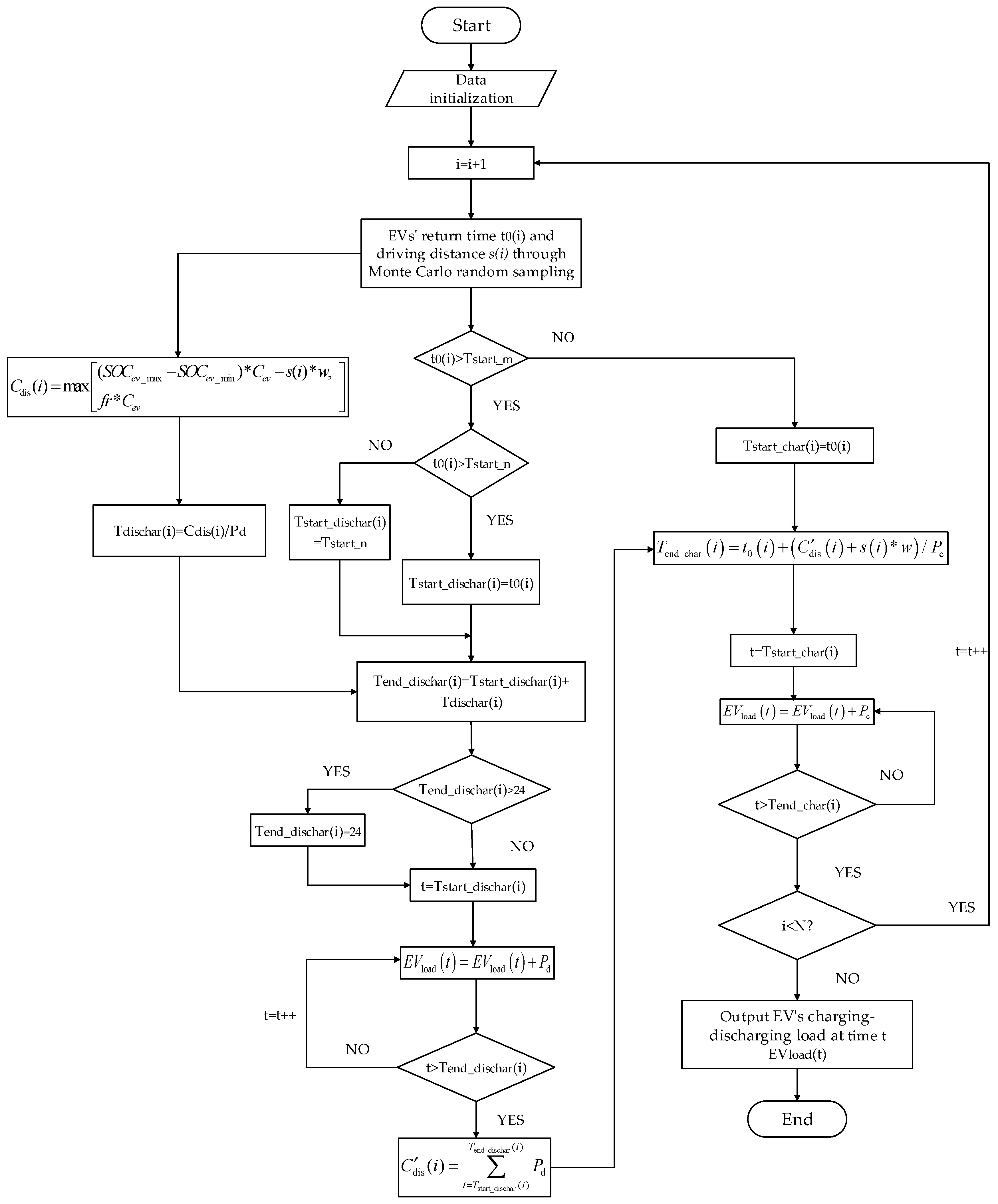
| EV charging-discharging load at time | |
| daily travel distance of EV | |
| daily travel distance of EV | |
| theoretical maximum discharging capacity of EV | |
| actual maximum discharging capacity of EV | |
| start-charging time of EV | |
| end-charging time of EV | |
| start-discharging time of EV | |
| end-discharging time of EV | |
| actual maximum discharging duration of EV | |
| COC of ES | |
| operation and maintenance ES cost | |
| charging and discharging conversion loss of ES | |
| small amount of charging cost of ES | |
| power output of ES at time | |
| power output of PV at time | |
| power output of WT at time | |
| MG load at time after load level optimization | |
| net load of the MG at time | |
| original load of MG system | |
| operation cost coefficient of the ES | |
| battery loss cost caused by the charge-discharge state change of ES | |
| replacement cost of the ES | |
| maximum SOC of the ES | |
| minimum SOC of the ES | |
| number of charge-discharge conversions in one cycle | |
| rated charge-discharge number in a life cycle | |
| maximum power output of ES | |
| minimum power output of ES | |
| COC of DE | |
| operation and maintenance cost of DE | |
| fuel cost of DE | |
| environmental pollution control cost of DE | |
| start-up cost of DE | |
| COC of main grid connect-line power | |
| electricity cost produced by the power exchange between the main grid and MG | |
| environmental pollution control cost | |
| power output of DE at time | |
| connect line of main grid at time | |
| operation cost coefficient of DE unit | |
| emissions of type pollutants generated by the operation of DE | |
| emissions of type pollutants generated by the operation of main grid connect line | |
| cost for handing type pollutants. | |
| fuel coefficients of DE | |
| cost of each start for DE | |
| number of start-up times of DE in one cycle | |
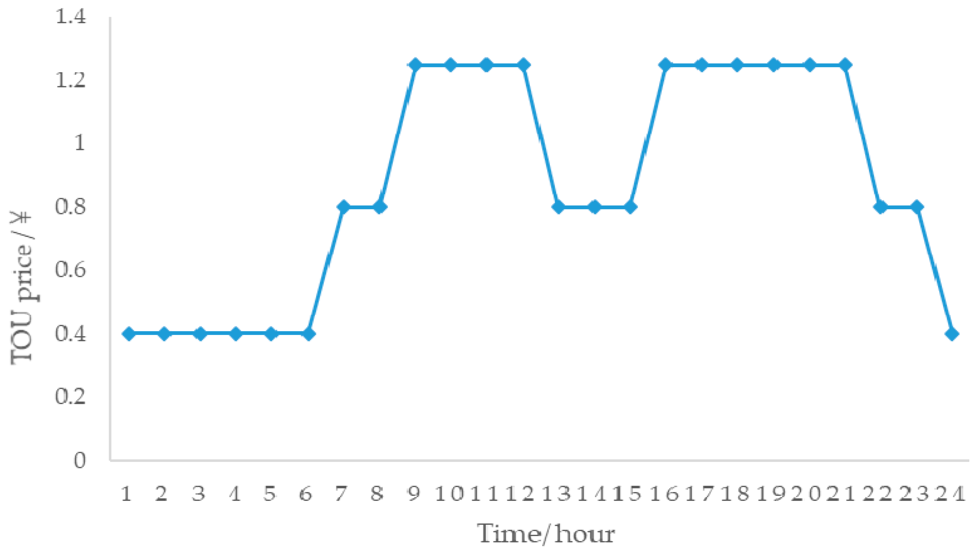
| TOU price at time of main grid side | |
| maximum power output of DE unit | |
| minimum power output of DE unit | |
| maximum climbing power of DE unit | |
| minimum climbing power of DE unit | |
| maximum power output of connect line of main grid | |
| minimum power output of connect line of main grid | |
| loss of load at time | |
| population size of MPSO | |
| particle dimension of MPSO | |
| population evolution iterations of MPSO | |
| position of particle at dimension | |
| velocity of particle at dimension | |
| particle’s individual optimum | |
| particle’s global historical optimum | |
| inertia weight of MPSO | |
| acceleration factor | |
| random number | |
| individual optimum value of the dimension at iteration | |
| global historical optimum value of the dimension at iteration | |
| Pareto optimal solution | |
| maximum value of the subobjective function | |
| minimum value of the subobjective function | |
| numbers of Pareto solutions | |
| numbers of subobjective function | |
| satisfactory degree for the subobjective function | |
| overall satisfactory degree for all objective functions |
Appendix A

| Operation Parameters | Items | ||||
|---|---|---|---|---|---|
| EV | ES | DE1 | DE2 | Main Grid Connect Lines | |
| Maximum output/ | 4 | 250 | 600 | 800 | 2000 |
| Minimum output/ | −4 | −250 | 0 | 0 | −600 |
| Maximum climb/ | / | / | 100 | 150 | / |
| Minimum climb/ | / | / | −100 | −150 | / |
| Charging efficiency | 0.9 | 0.9 | / | / | / |
| Discharge efficiency | 0.9 | 0.9 | / | / | / |
| Maximum SOC | 0.9 | 0.9 | / | / | / |
| Minimum SOC | 0.3 | 0.2 | / | / | / |
| / | 0.1040 | 0.236 | 0.236 | / | |
| Types of Pollutants | ||||
| Cost of Pollutant Disposal/ | 0.210 | 14.824 | 62.964 | |
| Coefficient pollutant emission/ | PV | 0 | 0 | 0 |
| WT | 0 | 0 | 0 | |
| DE | 649 | 0.206 | 9.89 | |
| Main grid | 889 | 1.8 | 1.6 | |
References
- Katiraei, F.; Iravani, M.R. Power management strategies for a microgrid with multiple distributed generation units. IEEE Trans. Power Syst. 2006, 21, 1821–1831. [Google Scholar] [CrossRef]
- Huang, W.T.; Yao, K.C.; Wu, C.C.; Chang, Y.R.; Lee, T.D.; Ho, Y.H. A three-stage optimal approach for power system economic dispatch considering microgrids. Energies 2016, 9, 976. [Google Scholar] [CrossRef]
- Wang, L.J.; Xu, H.L.; Wang, G. Economic dispatch model for microgrid considering power characteristics of distributed generators. Autom. Elec. Power Syst. 2016, 11, 31–38. [Google Scholar] [CrossRef]
- Augustine, N.; Suresh, S.; Moghe, P.; Sheikh, K. Economic dispatch for a microgrid considering renewable energy cost functions. In Proceedings of the 2012 IEEE PES Innovative Smart Grid Technologies, Washington, DC, USA, 16–20 January 2012. [Google Scholar]
- Ramabhotla, S.; Bayne, S.; Giesselmann, M. Economic dispatch optimization of mg in islanded mode. In Proceedings of the Energy and Sustainability Conference, Farmingdale, NY, USA, 23–24 October 2014. [Google Scholar]
- Wu, X.; Wang, X.L.; Wang, J.X.; Bie, Z.H. Economic generation scheduling of a microgrid using mixed integer programming. Proc. CSEE 2013, 28, 1–8. [Google Scholar] [CrossRef]
- Wu, H.; Wang, Y.S. Economic dispatch of microgrid using intelligent single particle optimizer algorithm. Power Syst. Prot. Control 2016, 20, 43–49. [Google Scholar] [CrossRef]
- Wang, X.H.; Qian, W.S. A new scheduling method of microgrid based on improved pso algorithm. Power Syst. Clean Energy 2017, 7, 53–57. [Google Scholar]
- Wang, Y.S.; Song, Y.Y.; Wu, H.; Yi, J.B. Security and economic dispatch of source/load for micro-grid based on Tabu search algorithm. Power Syst. Prot. Control 2017, 20, 21–27. [Google Scholar] [CrossRef]
- Chen, J.; Yang, X.; Zhu, L.; Zhang, M.X.; Li, Z.K. Microgrid multi-objective economic dispatch optimization. Proc. CSEE 2013, 19, 57–66. [Google Scholar] [CrossRef]
- Mao, M.Y.; Ji, M.H.; Dong, W. Multi-objective economic dispatch model for a microgrid considering reliability. In Proceedings of the 2nd International Symposium on Power Electronics for Distributed Generation Systems, Hefei, China, 12 August 2010. [Google Scholar]
- Farzin, H.; Fotuhi-Firuzabad, M.; Moeini-Aghtaie, M. A stochastic multi-objective framework for optimal scheduling of energy storage systems in microgrids. IEEE Trans. Smart Grid 2017, 8, 117–127. [Google Scholar] [CrossRef]
- Wang, J.; Wang, L.L.; Gou, Y.; Sun, L.H.; Guan, Z.J. Microgrid economic dispatch method considering electric vehicles. Power Syst. Prot. Control 2016, 17, 111–117. [Google Scholar] [CrossRef]
- Zhao, X.Y.; Wang, S.; Wu, X.H.; Liu, J. Coordinated control strategy research of micro-grid including distributed generations and electric vehicles. Power Syst. Technol. 2016, 12, 3732–3740. [Google Scholar] [CrossRef]
- Li, J.; Niu, D.; Wu, M.; Wang, Y.; Li, F.; Dong, H. Research on battery energy storage as backup power in the operation optimization of a regional integrated energy system. Energies 2018, 11, 2990. [Google Scholar] [CrossRef]
- Liu, H.T.; Ji, Y.; Zhuang, H.D.; Wu, H.B. Multi-objective dynamic economic dispatch of microgrid systems including vehicle-to-grid. Energies 2015, 8, 4476–4495. [Google Scholar] [CrossRef]
- Zhang, H.C.; Hu, Z.C.; Song, Y.H.; Xu, Z.W.; Jia, L. A prediction method for electric vehicle charging load considering spatial and temporal distribution. Autom. Electr. Power Syst. 2014, 1, 13–20. [Google Scholar] [CrossRef]
- Liu, H.; Ji, Y.; Zhuang, H.D.; Wu, H.B. Multi-objective economic dispatch of microgrid system considering electric vehicles. Trans. China Electrotech. Soc. 2014, s1, 365–373. [Google Scholar] [CrossRef]
- Einan, M.; Torkaman, H.; Pourgholi, M. Optimized fuzzy-cuckoo controller for active power control of battery energy storage system, photovoltaic, fuel cell and wind turbine in an isolated micro-grid. Batteries 2017, 3, 23. [Google Scholar] [CrossRef]
- Agrawal, S.; Panigrahi, B.K.; Tiwari, M.K. Multiobjective particle swarm algorithm with fuzzy clustering for electrical power dispatch. IEEE Trans. Evol. Comput. 2008, 12, 529–541. [Google Scholar] [CrossRef]
- Jin, N.; Rahmat-Samii, Y. Advances in particle swarm optimization for antenna designs: Real-number, binary, single-objective and multiobjective implementations. IEEE Trans. Antennas Propag. 2007, 55, 556–557. [Google Scholar] [CrossRef]
- Yang, Y.; Wu, J.F.; Zhu, X.B.; Wu, J.C. A hybrid evolutionary algorithm for finding pareto optimal set in multi-objective optimization. In Proceedings of the 2011 Seventh International Conference on Natural Computation, Shanghai, China, 26–28 July 2011. [Google Scholar]
- Xu, Y.; Dong, Z.; Xiao, C.; Zhang, R.; Wong, K. Optimal placement of static compensators for multi-objective voltage stability enhancement of power systems. IET Gen. Trans. Dist. 2015, 9, 2144–2151. [Google Scholar] [CrossRef]
- Yu, S.W. Case analysis and Application of MATLAB Optimization Algorithm, 1st ed.; Tsinghua University Press: Beijing, China, 2014; pp. 156–174. [Google Scholar]
- Hou, H.; Ke, X.B.; Wang, C.Z.; Fan, H.; Lou, J.Y. Coordinated optimazation strategy for electric vehicles’ charging and discharging in different regions. High Volt. Technol. 2018, 0222, 648–654. [Google Scholar] [CrossRef]


| Items | Disorderly Charging | Orderly Charging-Discharging |
|---|---|---|
| COC of ES unit/¥ | 310.53 | 308.9 |
| COC of DEs/¥ | 13,794 | 7243.829 |
| COC of connect-line power/¥ | 30,414.38 | 13,127.618 |
| Power fluctuation of connect line/kW | 8336 | 6755 |
| Item | Isolated Grid | Connected Grid |
|---|---|---|
| COC of DE/¥ | 26,564.93 | 7243.8290 |
| COC of connect-line power/¥ | / | 13,127.618 |
| Compensation cost of loss load/¥ | 6095.94 | / |
| Total COC/¥ | 32,660.87 | 20,371.447 |
© 2018 by the authors. Licensee MDPI, Basel, Switzerland. This article is an open access article distributed under the terms and conditions of the Creative Commons Attribution (CC BY) license (http://creativecommons.org/licenses/by/4.0/).
Share and Cite
Hou, H.; Xue, M.; Xu, Y.; Tang, J.; Zhu, G.; Liu, P.; Xu, T. Multiobjective Joint Economic Dispatching of a Microgrid with Multiple Distributed Generation. Energies 2018, 11, 3264. https://doi.org/10.3390/en11123264
Hou H, Xue M, Xu Y, Tang J, Zhu G, Liu P, Xu T. Multiobjective Joint Economic Dispatching of a Microgrid with Multiple Distributed Generation. Energies. 2018; 11(12):3264. https://doi.org/10.3390/en11123264
Chicago/Turabian StyleHou, Hui, Mengya Xue, Yan Xu, Jinrui Tang, Guorong Zhu, Peng Liu, and Tao Xu. 2018. "Multiobjective Joint Economic Dispatching of a Microgrid with Multiple Distributed Generation" Energies 11, no. 12: 3264. https://doi.org/10.3390/en11123264
APA StyleHou, H., Xue, M., Xu, Y., Tang, J., Zhu, G., Liu, P., & Xu, T. (2018). Multiobjective Joint Economic Dispatching of a Microgrid with Multiple Distributed Generation. Energies, 11(12), 3264. https://doi.org/10.3390/en11123264