Optimization of Performance Parameter Design and Energy Use Prediction for Nearly Zero Energy Buildings

Abstract

Optimizing key parameters with energy consumption as the control target can minimize the heating and cooling needs of buildings. In this paper we focus on the optimization of performance parameters design and the prediction of energy consumption for nearly Zero Energy Buildings (nZEB). The optimal combination of various performance parameters and the Energy Saving Ratio (ESR)are studied by using a large volume of simulation data. Artificial neural networks (ANNs) are applied for the prediction of annual electrical energy consumption in a nearly Zero Energy Building designs located in Shenyang (China). The data of the energy demand for our test is obtained by using building simulation techniques. The results demonstrate that the heating energy demand for our test nearly Zero Energy Building is 17.42 KW·h/(m²·a). The Energy Saving Ratio of window-to-wall ratios optimization is the most obvious, followed by thermal performance parameters of the window, and finally the insulation thickness. The maximum relative error of building energy consumption prediction is 6.46% when using the artificial neural network model to predict energy consumption. The establishment of this prediction method enables architects to easily and accurately obtain the energy consumption of buildings during the design phase.

1. Introduction

The world is confronted with climate change and greenhouse gas emission issues [1]. Nowadays, the energy consumption in the building sector accounts for 40% of the world’s total energy consumption, which suggests huge energy saving potential. Therefore, it is essential to identify and investigate the main factors which can have the most significant impact on building energy consumption [2,3]. Additionally, not only can lower greenhouse gas emissions be delivered by reducing building energy consumption, but also the economic development, the innovation of clean technology, and the mitigation of environmental and public health issues can be promoted [4].

Hence, green and energy efficient buildings such as nearly Zero Energy Buildings (nZEB) have attracted governments’ attention, and various building energy conservation standards and regulations have been established and implemented across different countries. For example, the Passive House Standard is a sustainable construction standard, which has been called for its implementation and enforcement by all member states by 2021. On 17 November 2009 the European Parliament and the Council fixed 2020 as a deadline for all new buildings to be nZEBs [5]. The European Union has decided that by year 2020 the building energy consumption will be cut down by 20% and greenhouse gas emission by up to 20% [6]. For the first time, the Ministry of Housing and Urban-Rural Development has made a clear demand of nZEBs development, which envisages huge market demand and the broad prospects in China of promoting nZEBs actively, and the goal is 10 million m² by the end of 2020 compared with 500 thousand m² now. nZEBs show high thermal comfort and low energy consumption. The required energy in nZEB can be provided from a variety of renewable energy resources including energy from renewable sources produced on-site nearby. International Energy Agency joint Solar Heating and Cooling Task 40 and Energy Conservation in Buildings and Community systems Annex 52 titled ‘‘Towards Net Zero Energy Solar Buildings’’ is making an international effort on the standardization of the Net Zero Energy Building definition [7].

The parametric design of the program stage plays a key role in the shape and performance of the building, which is also the source of the building’s energy-saving design. The energy saving potential that exists in decision making at different stages of design will progressively reduce as construction progresses [8]. There are many factors that influence the energy consumption of buildings, during architectural concept design. The building characteristics include parameters relating to geometry, services, glazing, activity, site, construction year, and weather.

Wilde [9] surveyed 67 buildings, where 57% of the technical measures needed to be implemented during the planning and design stage in the application of 303 green building technologies. Since the potential of building energy conservation can be previewed and examined flexibly on the data of heating and cooling loads obtained through simulations at design stage, the optimization of building envelops through parametric design has been attracting much more attentions from the building research community [10]. Based on the literature, the influence factors of the building envelope can be generally categorized into four aspects, namely the outline dimension, orientation, glazing area and thermo-physical properties of the construction materials [11].

Musall et al. [12] have studied energy saving measures applied in net Zero Energy Buildings. Advanced thermal insulation, solar thermal domestic hot water heating and heat recovery are widely used in passive houses, followed by passive technologies such as advanced daylighting, sun shading, passive cooling or ventilation. Bajc et al. [13] constructed and optimized Trombe walls using different types of glazing on the outside of the wall. The Trombe wall is designed with openings with flaps in its concrete core. Temperature distribution under the influence of Trombe wall in both the concrete core and the room are simulated, as well as velocity fields. After that, an analysis of the energy conservation potential iwas conducted. Daouas [14] studied the optimum insulation thickness in walls, energy savings and payback period in Tunisian buildings based on both cooling and heating loads. Yearly transmission loads are rigorously estimated using an analytical method based on Complex Finite Fourier Transform. The result suggests that wall orientation only has a small influence on optimal insulation thickness. The south appears to be the most economical orientation, however the energy conservation reaches the maximum, 23.78 TND/m² , when the wall is east-oriented. Özkan D B et al. [15] have investigated the effect of external wall areas and window alternations on the optimal insulation thickness and heating energy demands. Besides, effects of different insulation thicknesses and fuel consumption on emission of pollutants such as CO₂ and SO₂ are also evaluated.

There are many similar studies on the impact of windows on energy consumption. Susorova et al. [16] evaluated the influence of various geometry factors on building energy performance, including window orientation, window to wall ratio, and room width to depth ratio. Energy simulations were performed for six climate zones in the United States using a commercial office building model created in Design Builder. The most energy-efficient solution is when the window-to-wall ratio (WWR) to the north is 20%–30%, and WWR to the south is 50%–80% in cold climates. Thalfeldt et al. [17] simulated a generic open-plan office single floor model. Cost optimal and most energy efficient facade solutions, including window properties, external wall insulation, WWR and external shading were determined. At the cost optimal performance level, the best energy performance was as follows: In the direction of south, east, and north, they have three panes without external shading; WWR is 23.9%; external wall insulation reaches 200 mm; in the north, WWR is 37.5%.

Evidently, low and nearly zero energy buildings will need more careful design to optimize the performance design parameters. Energy consumption data is the basis for promoting energy conservation in science. Using simulation software to aid program design is an effective solution. However, the dynamic calculation of parameter settings and the calculation process are too complicated and difficult to grasp for the general engineering staff. The calculation and analysis of various schemes still takes a long time, especially for architectural design optimization. That involves the performance evaluation of many groups of programs. It requires a tool during architectural concept design that quickly and accurately evaluates the performance of the architectural scheme.

Artificial neural networks (ANNs) have been widely used in many problem domains, such as computer vision, speech recognition, machine translation, social network filtering, playing board and video games and medical diagnosis. With its flexible structures and powerful ‘learning’ ability, ANNs has become one of the most popular artificial intelligence models in the prediction of building energy consumption. Inspired by the structure of interconnected neurons in human brain, ANNs demonstrates a superior performance in solving non-linear problems with high-dimensional datasets compared to other AI models [18]. The network is constructed with different layers of neurons, with output layer connected to input and hidden layers to formulate a directed, weighted graph. The network will then be trained repeatedly or recursively to leverage the input dataset and identify the reasonable weights distribution for all neurons in the network. The whole process of modifying weights and functions for activation is called learning, and governed by specific rules [19].

In order to identify the optimal solution from energy optimization functions and improve the accuracy and performance of data-driven energy modelling, Banihashemi [20] proposed a unified approach by introducing an improved hybrid energy objective function and integrating both ANN and Decision Trees, which expands the applicability and enables the model to deal with both continuous and categorical data. Paterson [21] explored an alternative way of predicting building energy consumption by using machine learning methods rather than following the traditional path of physics-based building performance simulation. In this presented model, previously collected thermal comfort and electricity consumption data subject to corresponding certain design parameters are used as inputs to train ANNs model. The mean absolute percentage errors of ANNs model are 22.9% and 22.5% for the prediction of thermal energy usage and electricity consumption respectively. Zhai [22] proposed a systematic model for the optimization of heating, ventilation, and air conditioning (HVAC) systems subject to two adversary fundamental requirements, the less energy consumption and the guarantee of indoor thermal comfort. The model is constructed based on extreme learning machines and neural networks. Then the well-trained models are subsidized by two metaheuristic algorithms, namely sparse firefly algorithm and sparse augmented firefly algorithm (AFA). With the assistance of AFA, the highest potential energy saving rate can reach up to 30% whereby the indoor thermal comfort can still be maintained reasonably well. Ahn [23] proposed another ANN-based control models which can explore and identify optimal parameter settings for supply air by taking into account both the air amount and its temperature simultaneously. Based on research results, the developed ANN controller can effectively avoid control errors by 88% and reduce the energy consumption by 2% compared to conventional on/off controllers.

The gap that is being addressed by this study is integrated design. The performance parameters included 12 parameters relating to geometry, glazing, activity, WWR, and envelope insulation. Integrated design is conducive to understanding the whole process of the project. ANN model is an energy consumption prediction model under the influence of multiple factors. The aim of this study is to optimize building design parameters and predict building energy consumption. The research aim can be achieved by following two major steps. In the first step, the geometric model of our test building was first established in SketchUp, and thermal zones being characterized and divided as well. Then, thermal properties are furnished into the model of the building and weather condition loaded in EnergyPlus. The optimal combination of various performance parameters and the Energy Saving Ratio (ESR) are studied on the basis of a large quantity of simulation data. The second step served to establish ANN model. ANNs were trained to predict the energy consumption of nZEB design. The training data included energy consumption gathered through energy simulation software and measured building characteristics.

The reminder of the paper is organized as follows: Section 2 describes the methodologies of the studies. Section 2.1 presents the description of nZEB about collected building characteristics and systems description. Section 2.2 gives an overview of ANN model. Section 3 presents the simulation results and analysis from the models developed. The results to validate the proposed technique are discussed in Section 4. Finally, Section 5 reports the conclusions and outlook for future studies.

2. Materials and Methods

EnergyPlus is currently United States Department of Energy flagship whole-building energy simulation engine developed with the active involvement of many participating individuals and organizations since 1995, and is posted open-source on GitHub [24]. First of all, a physical model of the nZEB was built in SketchUp, and then a HVAC system and control strategy were established in OpenStudio [25]. Finally, the IDF files containing technical data about the building envelope materials and HVAC system were imported into EnergyPlus for simulation and optimization of various performance parameters.

EnergyPlus is widely used as an effective and powerful tool among the HVAC research community and engineers to improve and optimize building performance at all stages based on the simulated results about the holistic performance measurements and compositions of sub-sector energy consumptions. OpenStudio is a powerful tool developed by National Renewable Energy Laboratory used for building performance analysis. As a plugin in SketchUp and a visualization interface for EnergyPlus, OpenStudio not only absorbs all merits in building modeling from SketchUp, but also greatly simplifies the modelling of HVAC systems with its abundant component libraries and visualized window. HVAC systems in OpenStudio are mainly divided into Air Loop and Plant Loop. Air Loop is composed of the whole heat exchanger, heating coil, cooling coil, and fan. Plant Loop is composed of hot water loop, cold water loop, and water-side loop.

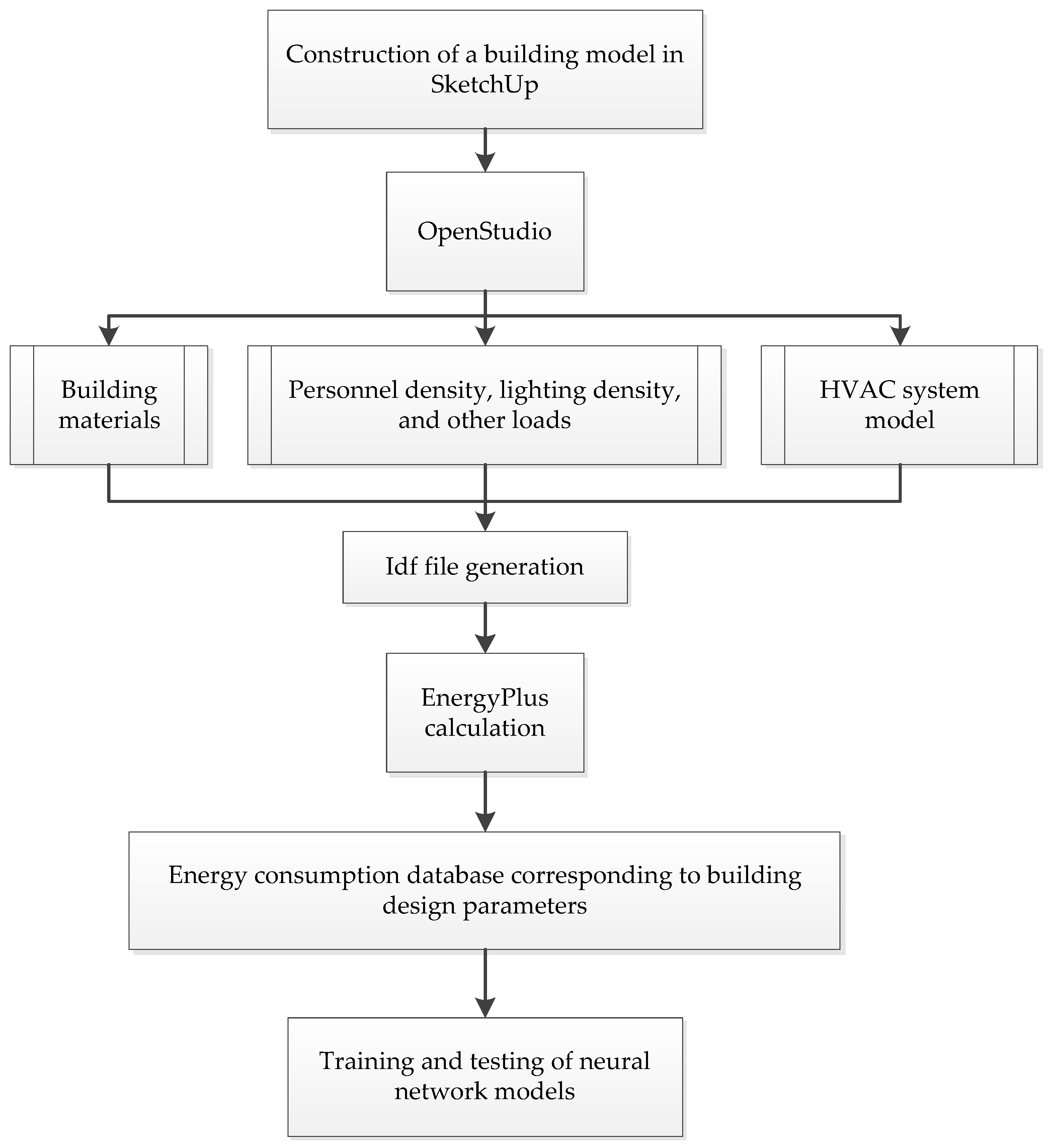
Building characteristics and systems description as well as the climate conditions are collected, and the geometric model was first established in SketchUp. The OpenStudio Application is a fully featured graphical interface to OpenStudio models including envelope, loads, schedules, and HVAC. Then, exported idf file is calculated in EnergyPlus. The impact of each variable on building energy consumption was analyzed through a large number of simulation calculations. The value of each key parameter is determined with energy consumption as a constraint. These 302 sets of data would be used as training and test data for the nZEB energy consumption forecasting model. A flow chart is given in Figure 1 to illustrate the analysis procedure of this study.

2.1. Description of the nZEB

2.1.1. Description of the research model

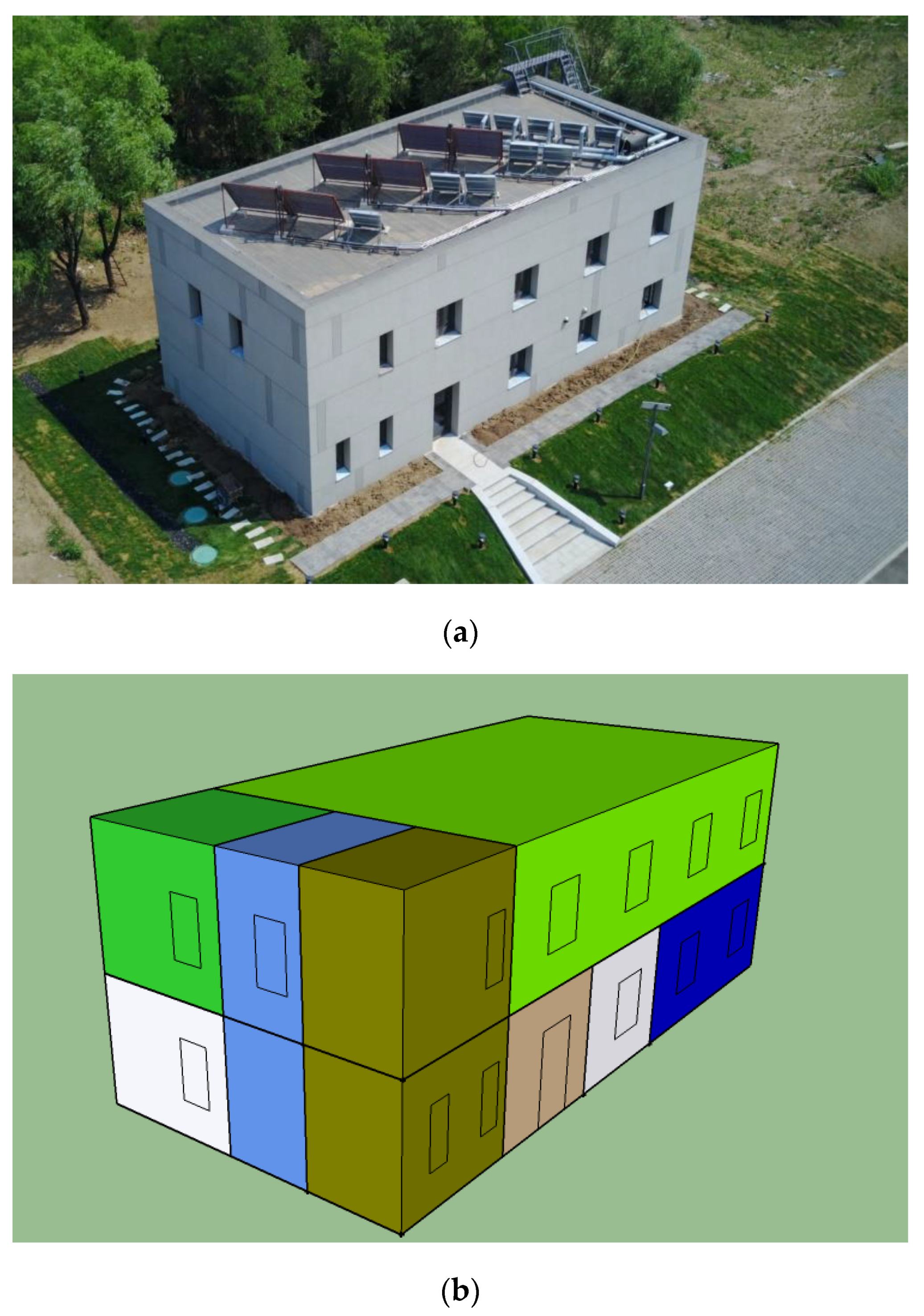
The Shenyang Jianzhu University nearly zero energy residential building demonstration center, shown in Figure 2a, is located in Shenyang, China.

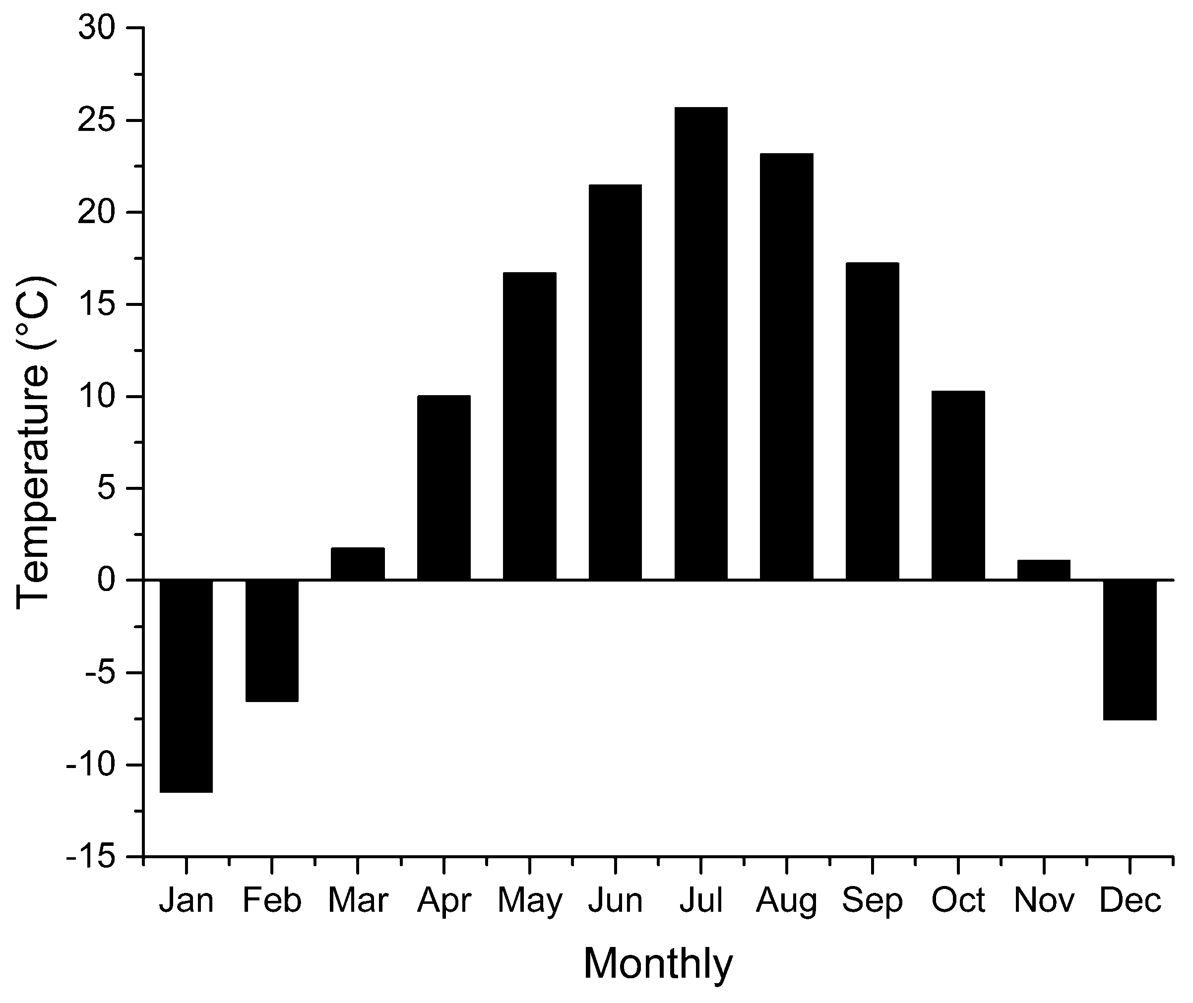
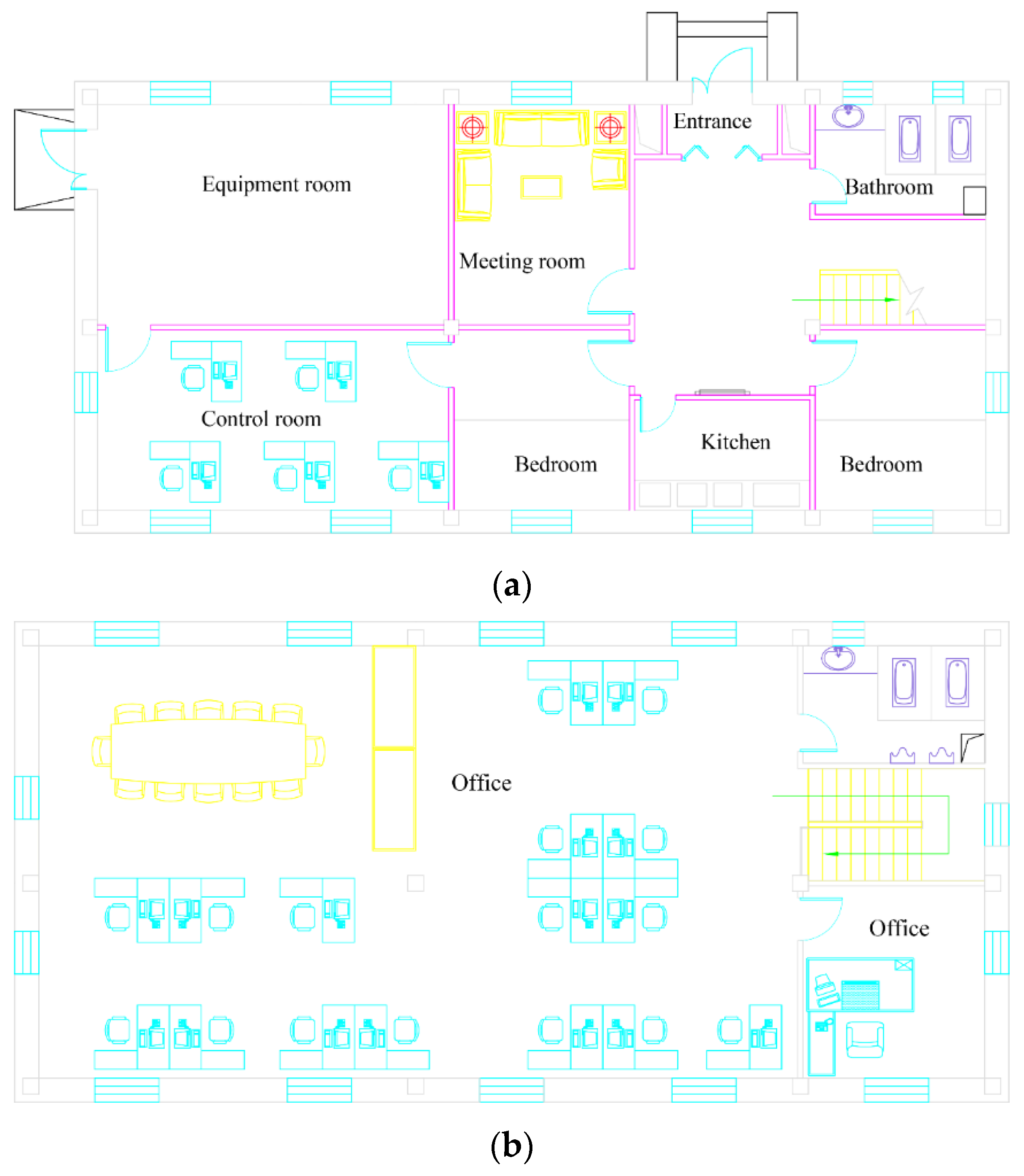
The climate zone is a cold climate zone. The building shape is rectangular. The main structure is an H-shaped steel structure with poured polystyrene foam concrete. The shape factor is 0.54, and the total area is 302.4 m². Figure 3 shows two floors. The space in first floor is occupied by a hall, equipment room, control room, bedroom, kitchen, bathroom and stairs, and the second floor by two offices and one toilet. Characterized as essential parameters for building performance and energy consumption, the heat transmission properties of each element of envelope (exterior wall, window, door, roof and ground floor.), are summarized in

Table 1. U values and thickness of each construction elements.

Component of Buildings	Elements of Construction	Thickness (mm)	U Value (W/m·k)
Exterior Wall	Polymer cracking mortar	5.00	0.930
	Expanded polystyrene board	300.00	0.033
	Self-insulation wall	120.00	0.100
	Calcium silicate board	10.00	0.240
	U value 0.099 [W/(m2·k)]
Roof	Waterproof materials	5.00	0.930
	Cement mortar	20.00	0.930
	Extruded polystyrene	280.00	0.028
	Autoclaved lightweight concrete	120.00	0.130
	U value 0.090 [W/(m2·k)]
Ground floor	Surface layer	20.00	0.930
	Concrete	100.00	1.300
	Extruded polystyrene	240.00	0.028
	Concrete cushion layer	80.00	1.300
	U value 0.113 [W/(m2·k)]
Windows	Low emissivity, filled Argon	-	-
	U value 1.0 [W/(m2·k)]

.

The geometric model of our studied building was established and thermal properties being characterized in SketchUp and EnergyPlus. Figure 2b depicts Thermal Zone in EnergyPlus simulation. The same function room is set as a thermal zone. The status of each thermal zone is always uniform, that is, the thermal zone of air temperature and humidity parameters are the same. Stairwell and the engine room are not set for heating or cooling, so they were set to non-air conditioning area, and the remaining thermal zone as air-conditioned area.

2.1.2. Building Systems Description

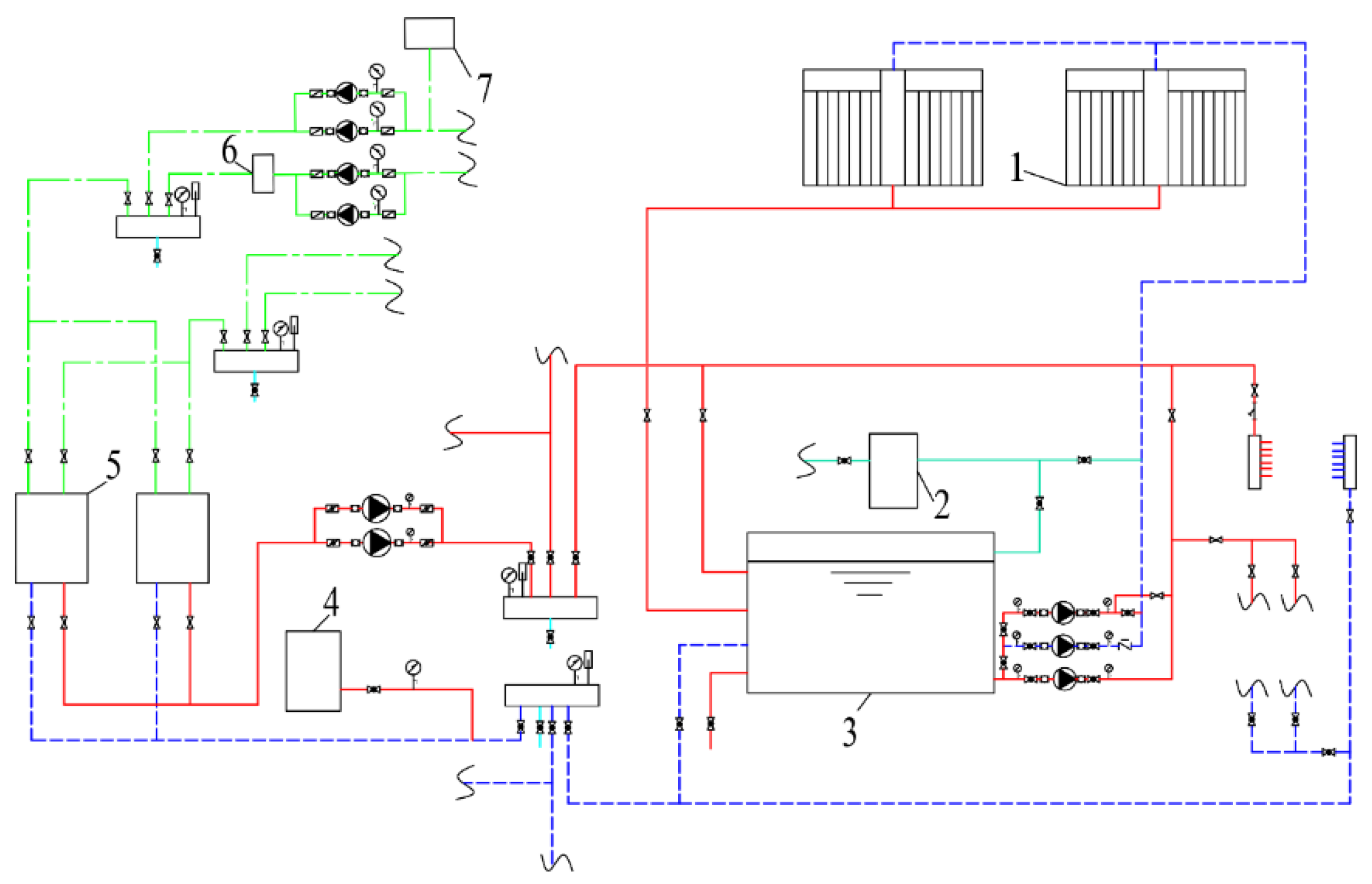
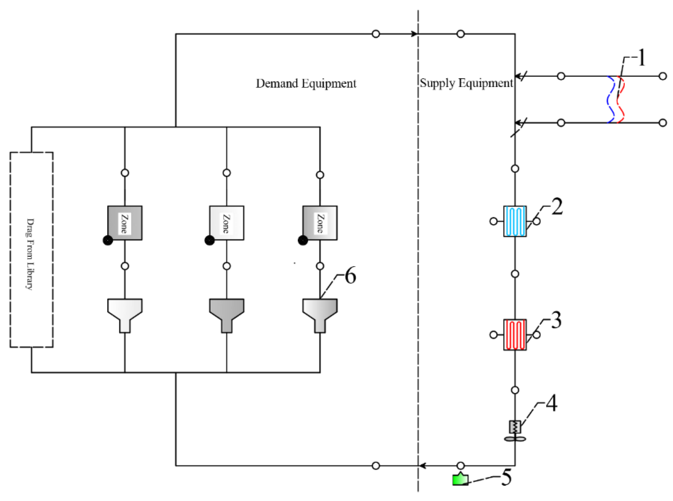
The system used in the nZEB for heating and cooling includes Water Source Heat Pump System, Solar Water Heating system, as shown in Figure 4.

The water source heat pump system bears most of the building’s heat load and full cooling load. The buried pipe outlet temperature is at 16 °C in summer, and the temperature difference between supply and return is 5 °C. The buried pipe outlet temperature is 12 °C in winter. The hot water loop provides hot water for a radiant floor heating system and the end of the heating coil in the air loop. Outlet temperature of hot water loop is 40 °C, and the temperature difference between supply and return is 8 °C. Also, there are several groups of solar collectors used for domestic hot water and heating. Mechanical Ventilation Heat Recovery Unit (MVHR) is the necessary system for nZEB [5]. It has 81% efficiency for sensible heat recovery and 73% efficiency for latent heat recovery. MVHR need not bear indoor heat load and moisture load. Fan open time is set to 8:00 to 21:00. Nighttime ventilation mode is turned on when the building has no heating or cooling needs. Figure 5 shows the MVHR.

2.2. ANN Approach

2.2.1. Overview

ANN models are effective when dealing with complex, nonlinear problems [26,27]. ANN’s are used for estimating heating/cooling loads, total electricity consumption and sub-level components’ operation and optimization [28]. The Back Propagation (BP) algorithm is the workhorse of learning in neural networks. BP algorithm trains a given feed-forward multilayer neural network for a given set of input patterns with known classifications [29]. As all instances from training dataset are inputted, the networks start to propagate forward till reaching the output layer, then output response according to the pattern of initial dataset will be compared with ground truth and the deviations being calculated. Based on the calculated deviations, the weights of neurons across the whole network will be calibrated and redistributed to mitigate the deviation, this process is considered as back propagation. 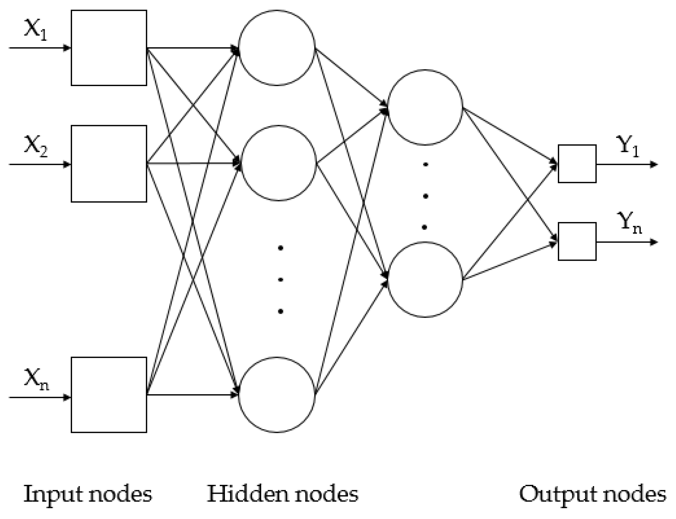BP algorithm [30] is based on Widrow-Hoff delta learning rule in which the weight adjustment is done through mean square error of the output response to the sample input. The sets of these sample patterns are repeatedly presented to the network until the error value is minimized. Three types of neurons in an ANN are shown in Figure 6; input nodes, hidden nodes, and output nodes [31].

MATLAB 7.13 was used to create the ANNs in this research [32]. Each neuron as one dimension in the input layer represents a parameter in the building characteristics dataset, and the single neuron in the output layer represents energy consumption. These data are given in

Table 2. Building characteristic parameters.

Parameter (Input Set)	Description Summary	Data Interval	Data Range
Exterior wall heat transfer coefficient	The proportionality constant between the heat flux and the thermodynamic driving force for the flow of heat	Insulation thickness, 20 mm	140–400 mm
Roof heat transfer coefficient		Insulation thickness, 20 mm	140–400 mm
Ground floor heat transfer coefficient		Insulation thickness, 20 mm	140–400 mm
Windows heat transfer coefficient		0.1 or 0.2 (W/m2·K)	0.6-1.1 (W/m2·K)
SHGC	Solar heat gain coefficient	It is up to the thermal performance of the window	It is up to the thermal performance of the window
window-to-wall ratio on east facades	The total area of all the east window openings divided by the east facades area	2.5%	5%–30%
window-to-wall ratio on west facades	The total area of all the west window openings divided by the west facades area	2.5%	5%–30%
window-to-wall ratio on south facades	The total area of all the south window openings divided by the south facades area	2.5%	5%–45%
window-to-wall ratio on north facades	The total area of all the north window openings divided by the north facades area	2.5%	5%–25%
Lighting	Indoor lighting electricity	1 W/m2	3–7 W/m2
electrical appliances	Indoor technology equipment electricity	1 W/m2	2–6 W/m2
personnel activities	Impact of personnel activities	1 m2/person	5-10 m2/person

.

2.2.2. Training

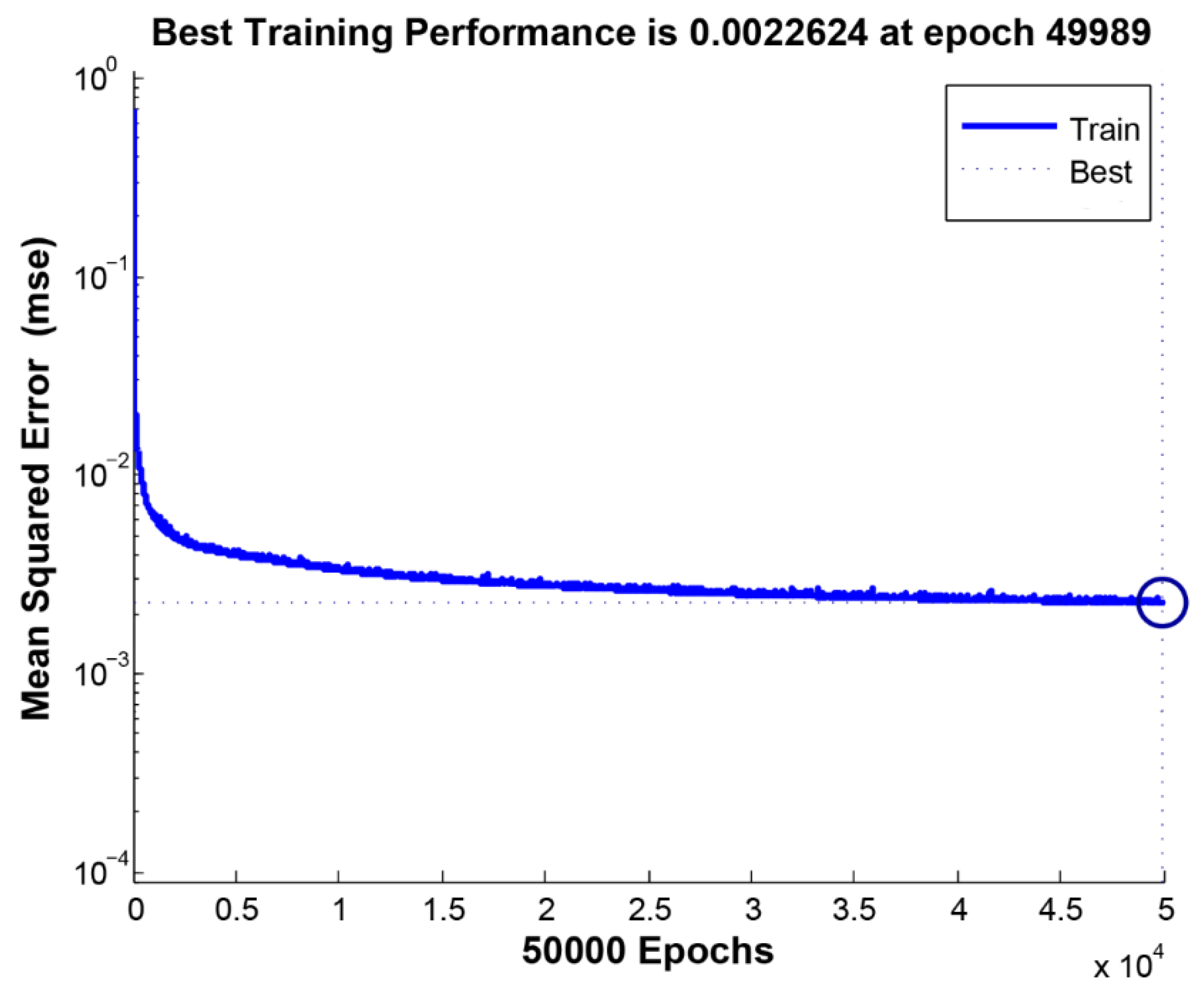
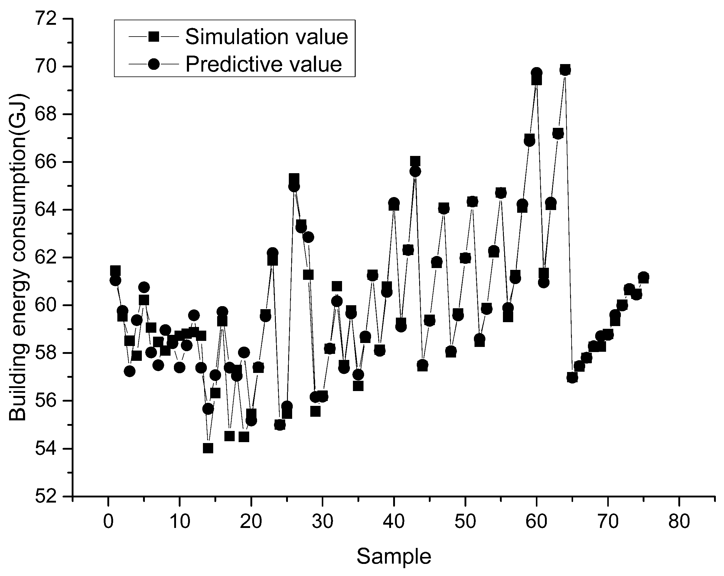
The whole data sets obtained from experiments are randomly divided into two parts for training and testing, respectively, thus 227 data sets are used as training data for the BP neural network model while 75 data sets are retained as testing data to validate the trained model. It should be noted that the divisions of data are formulated in a random manner and the cross validations are also applied to improve the ability of generalization of the model. Regarding limited volume of data samples, the model developing strategy adopted in this study can fully realize the potential of available data sets, therefore more likely to obtain a reasonable energy consumption predictive model under the topology of BP neural networks.

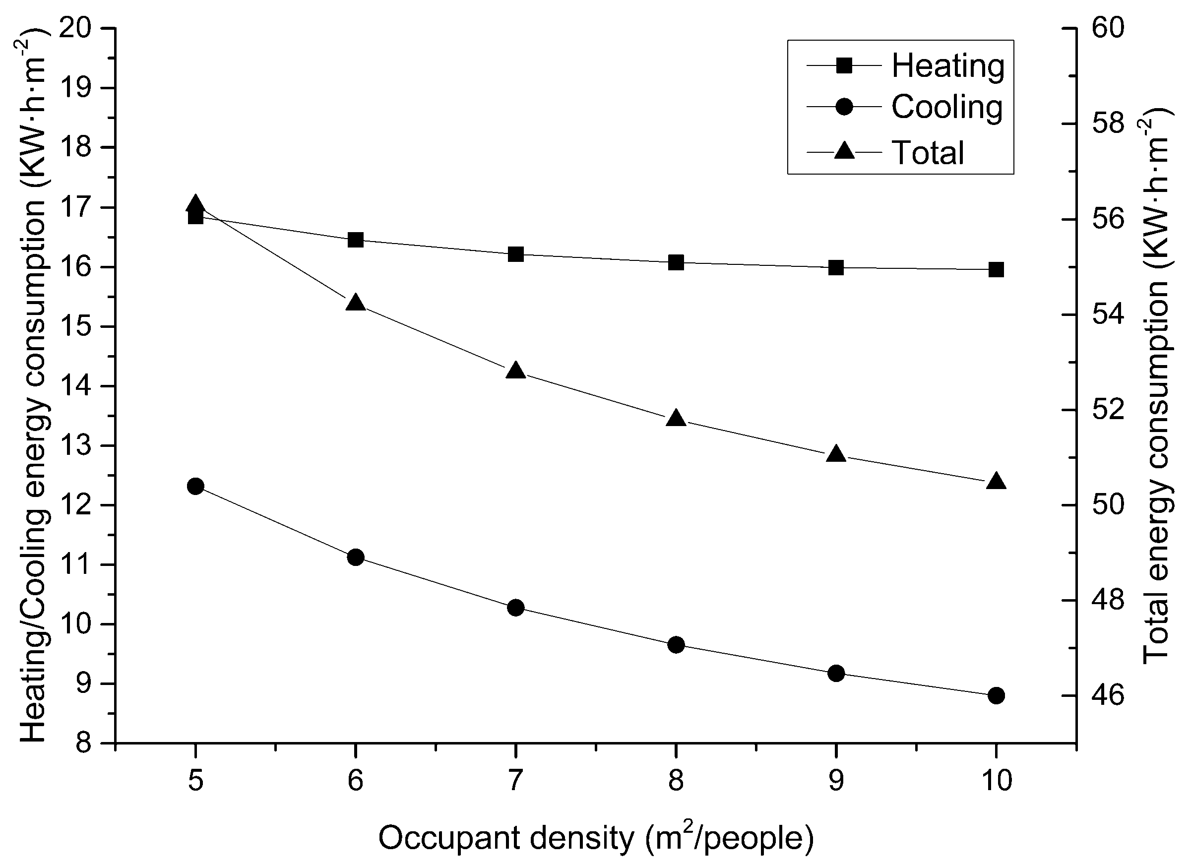
The input neurons of the established Back Propagation network model contain exterior wall heat transfer coefficient, roof heat transfer coefficient, ground floor heat transfer coefficient, windows heat transfer coefficient, solar heat gain coefficient (SHGC), WWR on east facades, WWR on west facades, WWR on south facades, WWR on north facades, indoor lighting, electrical equipment, and personnel activities. With twelve input variables required to predict energy consumption in this study, there are twelve neurons in the input layer corresponding to each variable. Similarly, as the sole purpose of this study is to predict building energy consumption, only one neuron is implemented in the output layer. The rest of the items were assigned the value of benchmark building when a certain performance parameter was changed to calculate the building energy consumption value.

Building energy consumption can be contributed by various factors including building construction, equipment, and occupancy characteristics and so on. A BP neural network with three layers is established in this study as an attempt to explore and quantify the possible relationship between various parameters and building energy consumptions. The input data are normalized into the scale of -1 to 1 based on Premnmx function provided in Matlab at preprocessing stage.

We use the newff function to create a feed-forward backpropagation network. The general syntax has been recorded in

Table 3. General syntax.

Net = Newff

net = newff (PR, [S1 S2 ... SNl], {TF1 TF2 ... TFNl}, BTF, BLF, PF) Description net = newff creates a new network with a dialog box. newff (PR, [S1 S2 ... SNl], {TF1 TF2 ... TFNl}, BTF, BLF, PF) takes, PR—R x 2 matrix of min and max values for R input elements Si—Size of ith layer, for Nl layers TFi—Transfer function of ith layer, default = ‘tansig’ BTF—Backpropagation network training function, default = ‘traingdx’ BLF—Backpropagation weight/bias learning function, default = ‘learngdm’ PF—Performance function, default = ‘mse’

[33]. The syntax of BP network is presented in

Table 4. BP network syntax.

net = newff (dx, [12-13-1], {‘tansig’, ‘tansig’, ‘purelin’}, ‘traingdx’);

Syntax: A = tansig (N) N: S-by-Q matrix of net input (column) vectors, the S-by-Q matrix of N’s elements squashed into [−1, 1]. Algorithms: tansig (n) = 2/(1 + exp(−2 ∗ n)) − 1

. In neural networks transfer functions are used to calculate a layer’s output from its net input. In this study the Hyperbolic Tangent Sigmoid Transfer Function (Tansig) is chosen as transfer function, while Traingdx is selected as training algorithm. Traingdx is a network training function that updates weight and bias values according to gradient descent momentum and an adaptive learning rate. The function traingdx combines adaptive learning rate with momentum training. Traingdx can be applied to train any network as long as its weight, net input, and transfer functions have derivative functions.

3. Results

3.1. Energy Consumption Simulation of Benchmark Building

The model built in OpenStudio mentioned in the previous paragraph was converted to the file (.idf). This file was loaded into EnergyPlus to run in Shenyang’s climatic conditions. To improve the predicting accuracy, the schedule of occupancy is extremely important since occupant behaviors can influence building energy consumption in a direct and intuitive way. Simulation was performed for a period of one year using a time step of 1 h. The schedule for different rooms of the entire building adopts the default value in EnergyPlus. Between 9:00 AM and 5:00 PM, the house is occupied, so that the energy consumed during this period of time is maximal. House heating starts in November and continues up to March (i.e. for 5 months), whereas, house cooling starts in June and continues up to August.

Another research interest in this study is to pinpoint the influence factors and their characteristics for each category of energy consumptions, including heating, cooling, lighting, electrical appliances, fans, water pump, and MVHR. A detailed analysis of the energy consumed by the nZEB was performed for the whole year.

Table 5. Energy consumption summary of benchmark building.

Statistical Classification	Heating	Cooling	Lighting	Electrical appliances	Fans	Water Pump	MVHR
Energy consumption KW·h/(m2·a)	17.42	9.77	8.62	8.43	2.34	4.81	2.54
The proportion of total energy consumption	32.31%	18.12%	15.97%	15.63%	4.34%	8.92%	4.70%
Total energy consumption KW·h/(m2·a)	53.93

illustrates the energy demand for each area separately for the nZEB simulated.

The total energy consumption for heating in nZEB was 5267.81 KW·h for the entire building surface of 302.4 m², which equals to17.42 KW·h/(m²·a) if divided by area. Another large portion of the energy is consumed by the cooling system in the house which is 9.77 KW·h/(m²·a), then followed by the lighting and electrical appliances.

The total energy demand is as low as 53.93 KW·h/(m²·a), which should be mainly accredited to the superb insulation of the house. Figure 7 displays average month temperature distribution for Shenyang, the minimum and maximum values of monthly temperature distribution. The highest annual temperature is 25.67 °C in July and the lowest temperature is −11.46 °C in January.

Additionally, Figure 8 presents temperature curve changes of the office on the second floor during the heating season. During the time it is occupied, the room temperature ranges between 19 °C and 22 °C. January is the coldest season in Shenyang.

3.2. Optimal Building Characteristic Parameters

3.2.1. Optimal Envelope Insulation Thickness

Technical guidelines [34] require heat transfer coefficient of exterior wall and roof of nearly zero energy residential buildings to be between 0.1 W/(m²·K) and 0.2 W/(m²·K). Heat transfer coefficient of ground floor is between 0.1 W/(m²·K) and 0.25 W/(m²·K).

Therefore, insulation thickness was set to 140–400 mm in EnergyPlus. The simulated variable step size was 20 mm. The exterior wall heat transfer coefficient corresponding to this setting was between 0.189 W/(m²·K) and 0.079 W/(m²·K). Roof heat transfer coefficient was between 0.164 W/(m²·K) and 0.065 W/(m²·K). Ground floor heat transfer coefficient was between 0.188 W/(m²·K) and 0.068 W/(m²·K). Heating energy dominates in total energy consumption no matter what the insulation thickness is, as shown in Figure 9. The total energy consumption does not exceed the 60 KW·h/(m²·a) specified in the technical guidelines when insulation thickness is between 140 mm and 400 mm.

It can be clearly seen from Figure 9 that with the increase in thickness of the external wall and the roof insulation, the total energy consumption shows a downward trend. The change curve of the external wall is more obvious, but the change in energy consumption with increase in the thickness of the ground insulation is relatively small. The impact of thickness of the exterior wall on energy consumption is the largest, followed by the roof thickness, and the last is thickness of the floor insulation.

3.2.2. Optimal Glazing Variants

The description of all glazing variants studied is shown in

Table 6. Typical windows summary of nZEBs in severely cold area.

Window Conding	U-value, W/(m2·K)	SHGC	Visible Light Transmittance	Tightness	Watertight	Wind Pressure	Initial Investment (yuan/m2)
A-P160	0.6	0.424	0.567	0.30/9 level	700/6 level	5000/9 level	5999
A-P120	0.8	0.439	0.629	0.30/9 level	700/6 level	5000/9 level	3999
B-PAS125	0.9	0.450	0.670	0.20/8 level	600/5 level	5000/9 level	2900
B-78	1.0	0.523	0.710	0.20/8 level	600/5 level	5000/9 level	2700
A-S86	1.1	0.533	0.650	0.30/9 level	700/6 level	5000/9 level	2599

. Technical guidelines stipulate that U-value of window is between 0.7 W/(m²·K) and 1.2 W/(m²·K). There are few windows with heat transfer coefficient lower than 1.2 W/(m²·K) in the market. We contacted different manufacturers to identify 5 windows used in nearly zero energy residential buildings. Among them, the first window has been produced but not applied.

Figure 10 shows that the total primary energy changed little when the U-value increased from 0.6 W/(m²·K) to 0.9 W/(m²·K). However, Table 6 shows that the price difference between the two is 3000 yuan/m². Change in energy consumption is very obvious when U-value increased from 0.9 W/(m²·K) to 1.0 W/(m²·K). In terms of cost, the difference between the two windows is 200 yuan/m².

3.2.3. Optimal WWR

As previous studies have shown, lowering WWR increases energy efficiency, but on the other hand it also reduces daylighting efficiency. Therefore, it is important to set lower limits to window sizes [17]. Design code for residential buildings (GB 50096-2011) states that daylight factor should not be below 1% in bedroom, living room (hall), and the kitchen. Furthermore, the daylight factor should not be below 0.5% when the light window is set near/on a staircase. Energy conservation design standard for heating in new residential buildings (JGJ26-2010) states WWR of each orientation. East and west WWR should be less than or equal to 30%. South WWR should be less than or equal to 45%. North WWR should be less than or equal to 25%. Simulated variables for WWR are shown in Table 2. East and west energy consumption curve is the steepest, followed by the south, while north energy consumption curve is the most gradual, as shown in Figure 11. This trend also represents the impact of WWR on energy consumption of nZEB in cold regions.

3.2.4. Indoor Thermal Disturbance

Not only objective design factors but also artificial subjective factors have an impact on energy consumption. This paper studies the effect of indoor thermal disturbance on the energy consumption of nZEB in cold regions. Indoor thermal disturbance includes staff density, lighting density and electrical appliances. Staff density was set to 5–10 m²/person in simulation according to the actual use of the building. The result is shown in Figure 12. With the reduction of indoor personnel, heating energy consumption, cooling energy consumption and total energy consumption all show a downward trend. The downward trend of heating energy consumption curve is relatively flat. Cooling energy consumption and total energy consumption are affected more.

The Technical Guide points out that the design value of lighting power density is 3 W/m². In addition, Heat generated by electrical appliances is 2 W/m². The effect of lighting density on energy consumption is shown in Figure 13. The lighting energy consumption is equal to the cooling energy consumption when the lighting density is 3.5 W/m². When the lighting density is 5.6 W/m², the lighting energy consumption is equal to the heating energy consumption. Although the energy consumption of heating decreased linearly at this time, the total energy consumption showed a straight upward trend. So the lighting density should be minimized under the conditions to satisfy the needs of indoor lighting.

Figure 14 depicts the effect of electrical appliances load on energy consumption. The impact of electrical appliances load is similar to lighting density. The electrical appliances’ energy consumption is equal to the cooling energy consumption when the electrical appliances load is 2.4 W/m². When electrical appliances load is 3.9 W/m², the electrical appliances’ consumption is equal to the heating energy consumption. The total energy consumption increases linearly with the increase of electrical appliances load. Therefore, the impact of electrical appliances cannot be ignored in design.

3.3. ANN Training

The BP network was trained and tested using the processed data in Section 2.2.2. Best training performance is 0.0022624 at epoch 49989. As shown in Figure 15, the network training is over when the function converges. The mean squared error (MSE) assesses the quality of an estimator or a predictor. Definition of an MSE differs according to whether one is describing an estimator or a predictor. For each fold, the ANN with the lowest mean squared error for the testing data was saved and the generalization errors were determined. MSE is given in Equation (1) [21]:

$$E\left(MSE\right)=\frac{1}{n}{\displaystyle \sum _{i=1}^n{\left(\stackrel{\wedge }{Y_i}-Y_i\right)}^2}$$

(1)

where $\widehat{Y}$_i is the target output, and Y_i is the predicted output, for the training, validation or testing data configuration i, and n is the total number of configurations in the training, validation, or testing data.

Figure 16 shows the BP neural network model training process. Degree of fitting between BP neural network training results and actual results is high after repeated training. This shows that BP network training meets the expected requirements. Then the test data was predicted using the trained BP network model. The result is shown in Figure 17. The maximum relative error of building energy consumption prediction is 6.46%. Prediction accuracy is high when using BP network model to predict energy consumption.

4. Discussion

The Ministry of Housing and Urban-Rural Development of the People’s Republic of China drew on the experience of foreign passive houses and nearly zero energy buildings, combined with the existing engineering practices in our country to compile the “Passive low energy consumption of green building technology guidelines” [34]. Shenyang is in a cold climate in China. In this cold climate such a building has the following characteristics:

• Annual space heat requirement of 18 KW·h/(m²·a);
• Total energy consumption for heating, cooling and lighting should not exceed 60 KW·h/(m²·a);
• Leaked air volume must not be higher than 0.6 of the house volume per hour as measured at a pressure of 50Pa;

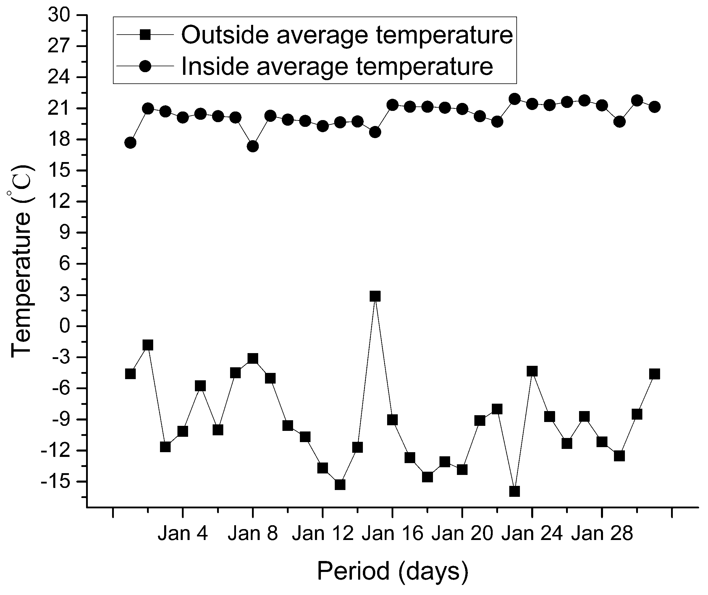
As is shown from Table 5, the heating energy consumption of the building in the annual energy consumption simulation results is 17.42 KW·h/(m²·a). This value is less than 18 KW·h/(m²·a). The annual building energy consumption is 53.93 KW·h/(m²·a). This value is also within the scope of the Technical Guidelines. Taking the open office area as an example, indoor average temperature reached 19–22 °C during heating in winter, as shown in Figure 8, which represents a comfortable temperature for the occupants. This nZEB possesses a high thermal inertia which in a way protects the indoor environment from the invasion of outdoor disturbance so as to maintain indoor temperature at a comfortable level for occupants, which further reduces the energy consumption induced by the requirement for heating. The energy demand of passive house in Bucharest was simulated using the energyplus software [6]. Building characteristics and system description are similar to benchmark building, including climatic conditions. Simulated demand of energy for heating was 14.1 KW·h/(m²·a).Bucharest ’s climate is milder than Shenyang, so heating demand is smaller.

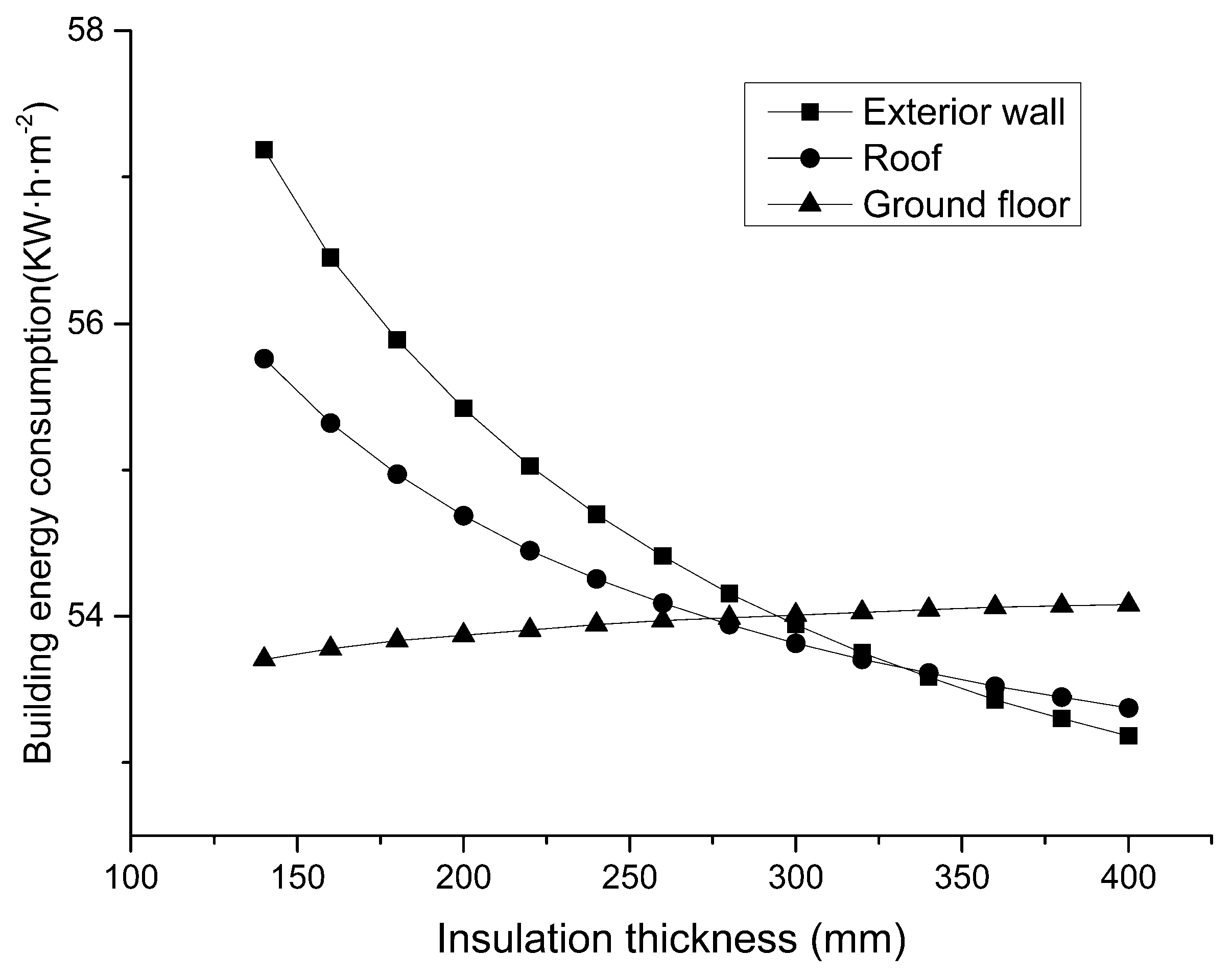
However, when the exterior wall insulation thickness is less than 260 mm, equivalent to the heat transfer coefficient being greater than 0.115 W/(m²·K), the heating energy consumption exceeds the required value of 18 KW·h/(m²·a). The same is true for the roof. When the roof insulation thickness is less than 220 mm, the energy consumption of heating will also exceed the standard value. Thus, it can be seen that even if the heat transfer coefficient of the exterior wall and roof meets the requirements of the technical guidelines, the energy consumption in the final operation may exceed the standard. Therefore, in the program design stage, we can’t blindly follow standard values, which may lead to excessive energy consumption.

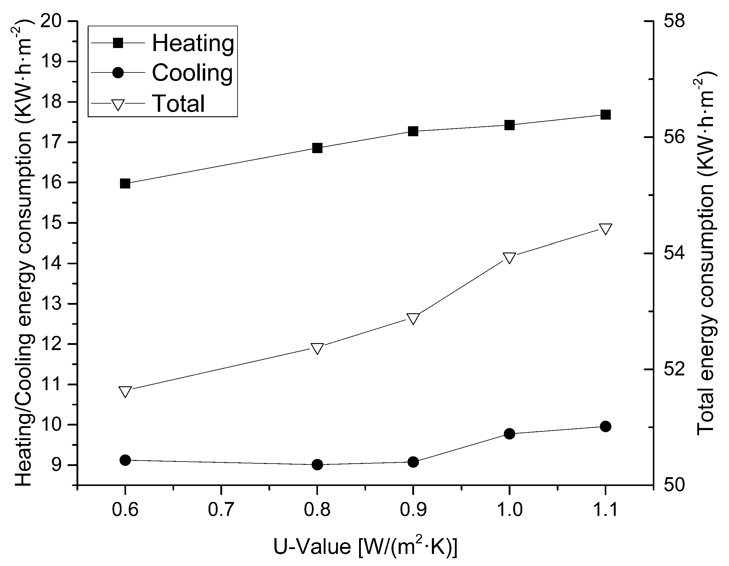
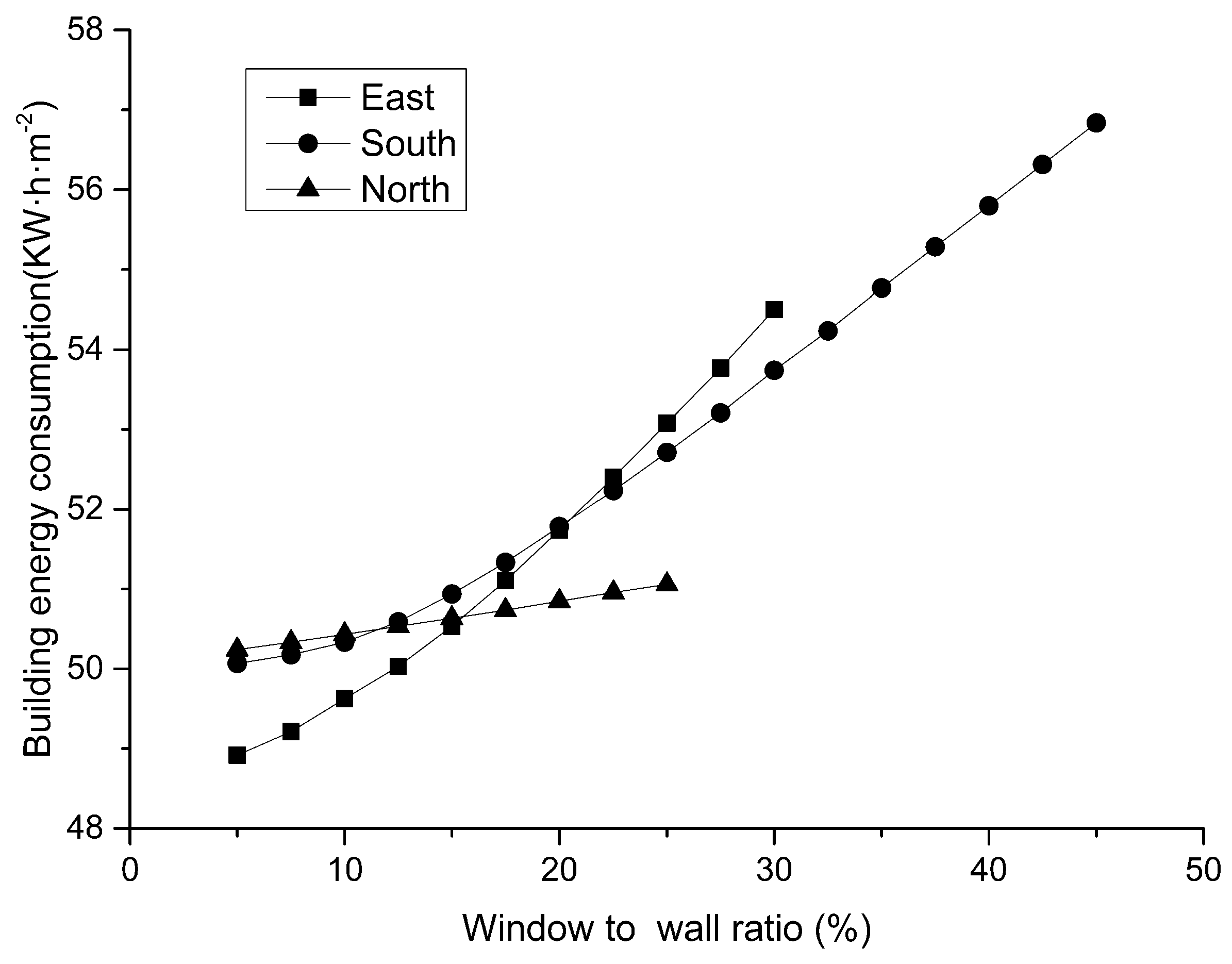
In any case, it is very important for economic evaluation to be run in parallel with energy simulations, as a cost-optimal solution can really change the design. PAS25 series of windows with U-Value of 0.9 W/(m²·K) would be the best choice from the cost optimal and energy efficient viewpoint. After simulation optimization, it can be seen that the WWR of each orientation in the scheme stage is 11.59%–15% in the east (west) direction and 9.93%–17.5% in the south direction. The WWR of north facade should try to take a small value on the premise of meeting lighting requirements and ventilation requirements. ESR has been introduced to quantitatively analyze the energy saving effect. In this paper, ESR is defined as Equation (2) [22]:

$$ESR(E_i)=\frac{E_i-E_{bench}}{E_{bench}}\times 100\%$$

(2)

where E_i is the energy consumption at given optimization parameter. E_bench is the benchmark energy consumption.

The benchmark energy consumption in Section 3.1 for heating, cooling, and electricity is 53.93 KW·h/(m²·a). E_i is the optimal energy consumption value after changing a key performance parameter. In this paper, the key parameters are as follows: exterior wall insulation thickness, roof insulation thickness, window thermal performance parameters, and WWR for each orientation of the building.

Table 7. Summary of optimizations results on ESR.

Parameters	Ranges	Ei [KW·h/(m2·a)]	ESR(Ei)
Exterior wall insulation thickness	280 mm	54.15	0.41
	300 mm	53.94	0.02
	320 mm	53.75	−0.33
Roof insulation thickness	260 mm	54.09	0.30
	280 mm	53.94	0.02
	300 mm	53.81	−0.22
Window thermal performance parameters	Similar PAS125	52.90	−1.91
WWR for East	12.5%	50.03	−7.23
	15%	50.53	−6.30
WWR for South	10%	50.33	−6.68
	12.5%	50.59	−6.19
	15%	50.94	−5.54
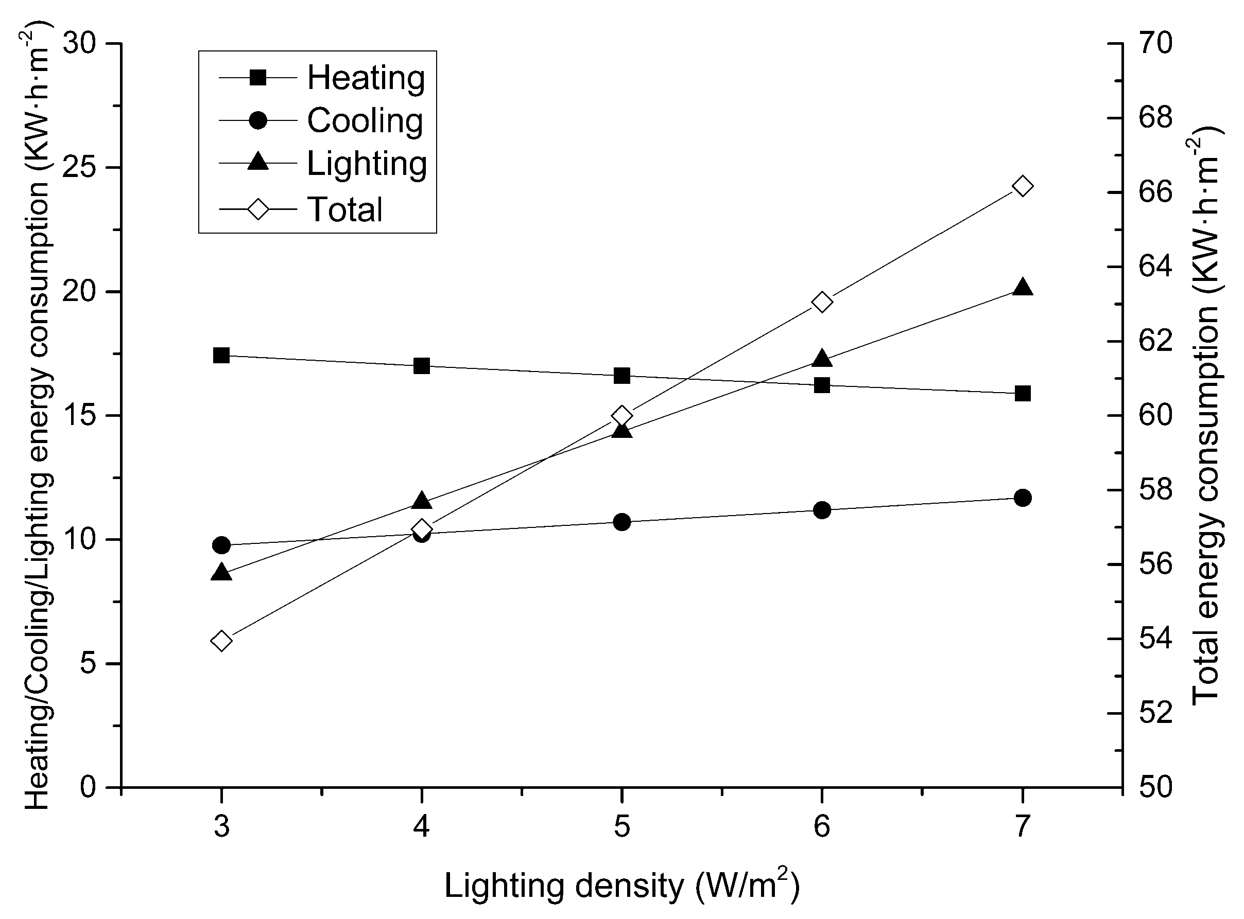
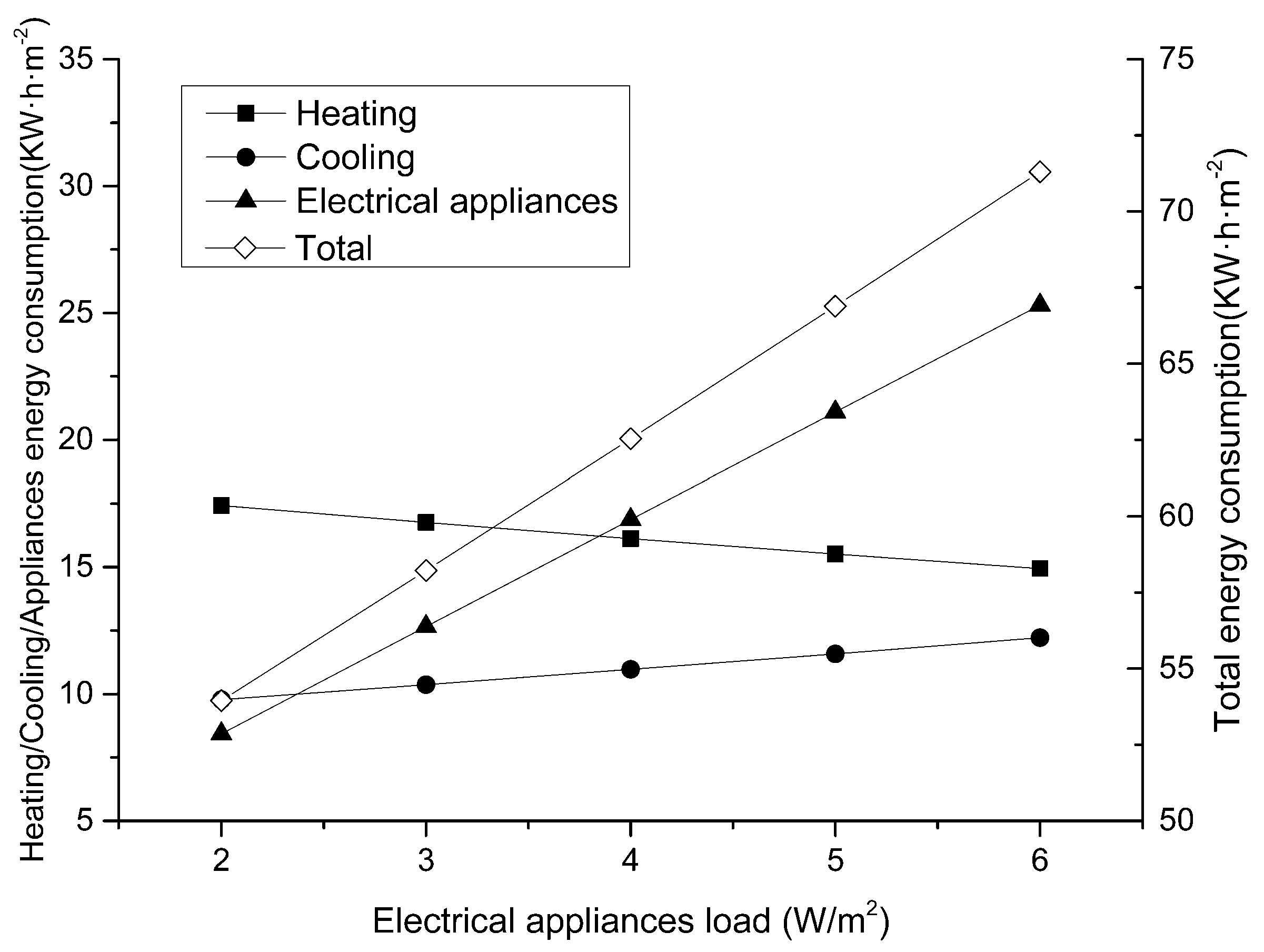
	17.5%	51.33	−4.82

shows that WWR optimization has the most significant potential for energy saving, followed by the window thermal performance parameters, and finally the envelope insulation thickness.

There is a great association with sample data whether prediction of the artificial neural network model is correct or not. The efficiency of network learning and the accuracy of prediction will be better when the sample data can better represent the characteristics of the predicted problem. On the other hand, when the noise of the sample is too much, the network will learn a lot of useless experiences, which greatly reduces the learning rate and affects the accuracy of the network prediction. The energy consumption of buildings is affected by several characteristics, such as geometry, services, glazing, activity, and weather. However, artificial neural network model has the characteristic of self-learning. It can be based on the different parameters of the building as an input, and then the neural network will automatically adjust the weight, thereby accurately predicting the building’s energy consumption.

The influence of the key performance parameters on the energy consumption of nZEB during the design stage was analyzed through EnergyPlus simulation. 302 sets of data were obtained as training and testing data of BP network model. At the same time, BP model input neurons were identified, including 12 variables: building envelope thermal performance parameters, window-to-wall ratios, indoor thermal disturbance, as shown in Table 2. There is one output neuron in the model, that is, annual energy consumption per unit area of construction. The training parameters of 3-layer BP neural network and network model are determined. 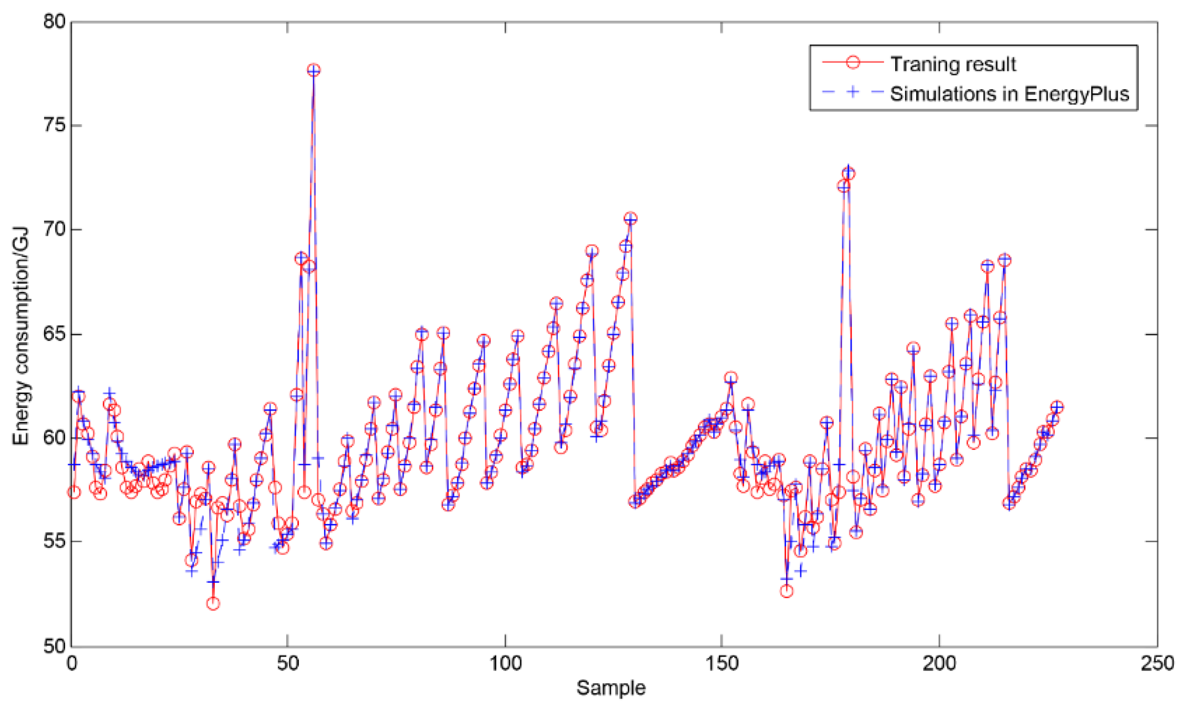Figure 17 shows that the model can predict the energy consumption better. Nearly zero energy buildings will need more careful design to promote energy conservation. The establishment of this prediction method enables architects to easily and accurately obtain the energy consumption of buildings during the design phase. We can adjust the design parameters at any time based on the prediction of energy consumption.

Kang [35] analyzed Equations for Energy Consumption Prediction using Analysis of Variance and multiple regression analysis.The tests also applied an EnergyPlus simulation. The criterion used for the improvement of the prediction was the coefficient of determination. It is expressed as a decimal number between 0.00 and 1.00. 1.00 means perfect prediction in the model. This coefficient is 0.753 for heating energy consumption and 0.602 for cooling energy consumption.

5. Conclusions

This paper presents a study of the nZEB, built in China’s cold climate conditions, in accordance with the passive low energy consumption of green building technology guidelines. This nearly zero energy building demonstrates a high thermal inertia which in a way protects the indoor environment from the invasion of outdoor disturbance so as to maintain indoor temperature at a comfortable level for occupants, which further reduces the energy consumption induced by the requirement for heating. Key performance parameters in architectural design stage were optimized based on nZEB energy requirements. The optimal combination of various performance parameters and the ESR were studied on the basis of a large quantity of simulation data. These data were used as training data for artificial neural networks. ANNs were trained to predict the energy consumption of nZEB design.

The heating energy consumption of the building in the annual energy consumption simulation results is 17.42 KW·h/(m²·a), which is the dominant factor in total building energy consumption. The annual building energy consumption is 53.93 KW·h/(m²·a). These values are also within the scope of the Technical Guidelines. This building maintains good thermal comfort while meeting energy efficiency standards. We get the following conclusions for the optimization of key performance parameters.

The optimal thickness of exterior wall insulation is 280-320 mm, and corresponding total annual energy consumption is 53.75–54.15 KW·h/(m²·a). The ESR is about 0.33%. The optimal thickness of roof insulation is 260-300 mm, and corresponding total annual energy consumption is 53.81–54.09 KW·h/(m²·a). The ESR is about 0.22%. The typical window optimization results are similar to the B-PAS125, and corresponding total annual energy consumption is 52.90 KW·h/(m²·a). The ESR is about 1.91%. The optimal WWR for the east or west is 12.5%–15%, and corresponding total annual energy consumption is 50.03–50.53 KW·h/(m²·a). The ESR is about 7.23%. The optimal WWR for the south is 10–17.5%, and corresponding total annual energy consumption is 50.33–51.33 KW·h/(m²·a). The ESR is about 6.68%. In terms of energy saving potential, this shows that the energy-saving effect of WWR optimization is the most obvious, followed by thermal performance parameters of the window, and finally the insulation thickness.

The maximum relative error of building energy consumption prediction is 6.46%. Prediction accuracy is high when using BP network model to predict energy consumption. The neural network model’s calculation process is relatively simple compared with the dynamic calculation method. Therefore, it is easier for engineering designers to learn and apply. In addition, the target optimization process involves a large number of iterative calculations. The energy consumption of the building needs to be evaluated for each iteration. This method takes less time than the dynamic calculation method. The establishment of this prediction method enables architects to easily and accurately obtain the energy consumption of buildings during the design phase.

Additionally, the Ministry of Housing and Urban-Rural Development of the People’s Republic of China has mandated that more than 10 million square meters of ultra-low energy consumption, nearly zero energy building demonstration projects will be completed by the year 2020. This study provides essential information that can be used in the future for nZEBs or energy-efficient buildings that will be built in cold climates in China.

In the future, thermal comfort of the nZEBs will be considered. Air temperature, mean radiant temperature, relative humidity, air velocity, dressing style, human activity will be designed. Multi-objective optimization will also be carried out.