Energy and Economic Analysis for Greenhouse Ground Insulation Design

Abstract

Energy and life cycle cost analysis were employed to identify the most-cost effective ground envelope design for a greenhouse that employs supplemental lighting located in Ottawa, Ontario, Canada (45.4° N). The envelope design alternatives that were investigated consist of installing insulation vertically around the perimeter and horizontally beneath the footprint of a greenhouse with a concrete slab and unfinished soil floor. Detailed thermal interaction between the greenhouse and the ground surface is achieved by considering 3-dimensional conduction heat transfer within the TRNSYS 17.2 simulation software. The portion of total heat loss that occurred through the ground was approximately 4% and permutations in ground insulation design reduced heating energy consumption by up to 1%. For the two floor designs, the highest net savings was achieved when perimeter and floor zone horizontal insulation was installed whereas a financial loss occurred when it was also placed beneath the crop zone. However, in all cases, the improvement in economic performance was small (net savings below $4000 and reduction in life cycle under 0.2%). Combined energy and life cycle cost analysis is valuable for selecting optimal envelope designs that are capable of lowering energy consumption, improving economics and enhancing greenhouse durability.

1. Introduction

Heating is a major operating expense for greenhouses that are located in mid-to-high latitude locations. In addition, heating is commonly achieved by burning fossil fuels, which contribute to greenhouse gas emissions and environmental degradation. Since most of heat loss occurs through the envelope (walls, roof and floor), optimal designs, which reduce energy use while addressing economics concerns, are required.

Much of the prior work regarding ground heat transfer has been performed for buildings [1,2,3] whereas only a few studies have been performed for greenhouses. Most of the research for greenhouses ground heat transfer consists of case studies [4,5,6] or the potential for design improvements such as ground-source heat exchangers [7,8]. Various levels of modeling resolution have been employed for representing the thermally massive ground. Most studies have separated the ground into one or more relatively thin earth layer and energy transfer is solved using 1-dimensonal (1D) heat transfer equations [9,10,11]. The advantage of 2-dimensional (2D) heat transfer is that it enables interaction with the greenhouse edge/perimeter. For instance, a numerical study using computational fluid dynamics enables visualization of the ground temperature profile [12]. However, the entire footprint (and interaction with the perimeter) can only be studied when 3-dimensional (3D) discretization of the ground is performed, whereby the ground is divided into control volumes so that overall heat transfer can be solved analytically or numerically. The only study that employed 3D analysis of ground heat transfer in greenhouses used the WUFI software to compare thermal energy use for a greenhouse located above, below and at ground level [13]. However, these studies did not consider economic implications of employing ground insulation. To determine the most cost-effective design, a combined energy and economic analysis must be performed. To our best knowledge, there has not been any previously published work regarding the detailed 3D energy analysis and economic analysis for the design of a greenhouse floor envelope.

The aim of this paper is to demonstrate how integrated thermal-daylight energy analysis and life cycle cost analysis (LCCA) can be employed to identify the most-cost effective ground insulation design for a greenhouse that controls light to a consistent daily integral located in Ottawa, Ontario, Canada (45.4° N, mid-latitude, 4560 heating degree-days).

2. Energy and Economic Analysis

For greenhouses that supplement daylight with horticultural lighting, the choice of cover materials may alter the daylight availability and lighting electricity use. The effect of such alterations must be transferred to the module which calculates the thermal energy consumption. In theory, modifying the envelope design for greenhouses that control light to a consistent daily integral (e.g., for producing leafy green vegetables year-round near the consumer) should not affect crop growth as the supplemental lighting and heating system control will adjust and compensate for any changes in the indoor climate. Consequently, the analysis of this type of greenhouse will be carried out by omitting biological aspects.

The decision-making process for envelope design requires both energy and economic analysis. The performance obtained through energy simulation is not sufficient for determining a cost-optimal design. From an investor’s perspective, the incremental cost of alternative claddings should be outweighed by operational savings. This study employs LCCA and the net savings method was selected for comparing envelope design alternatives. The net savings method can provide detailed economic analysis in a time efficient manner (it only requires economic aspects that are impacted by a design variation to be quantified).

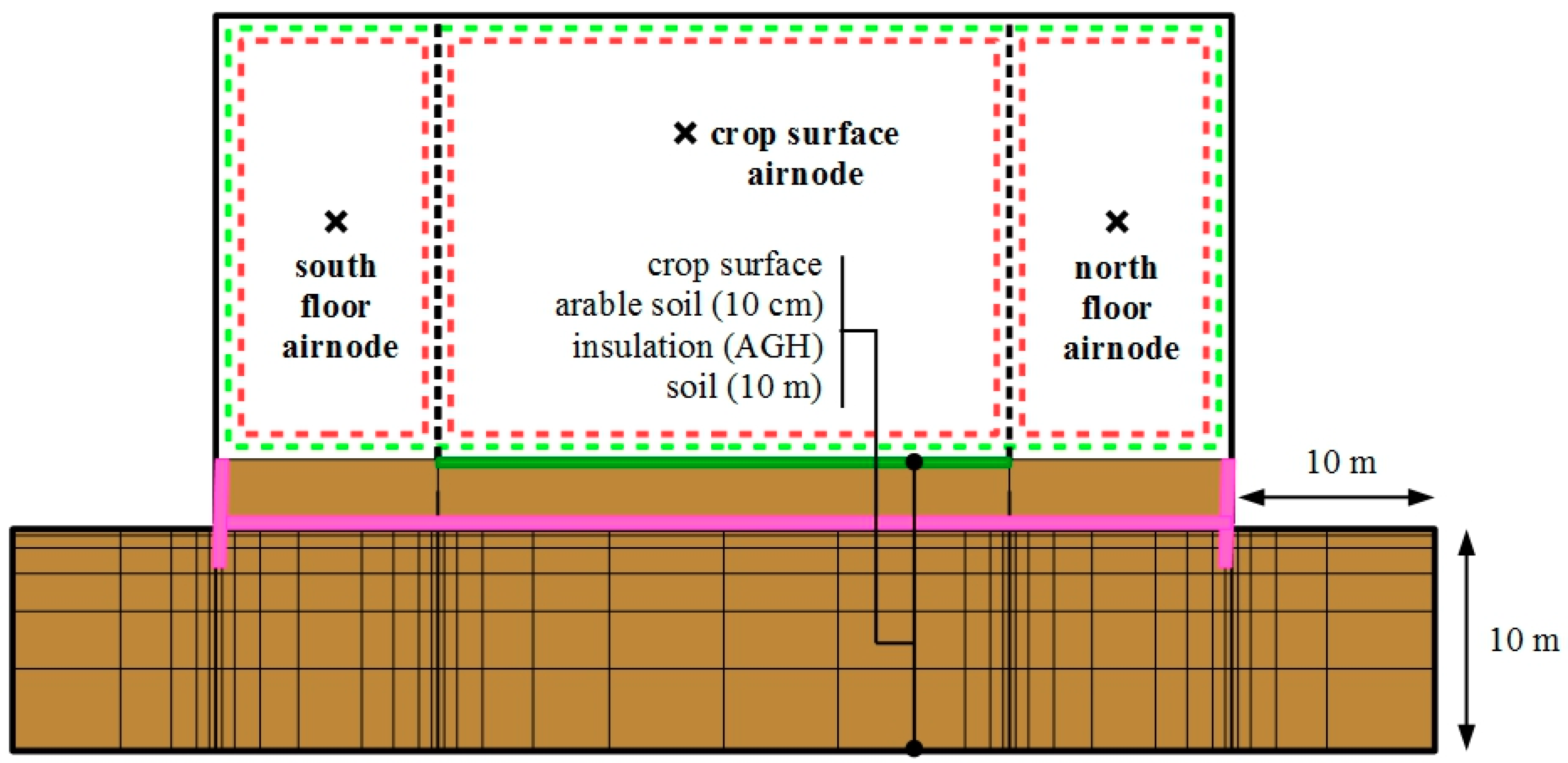
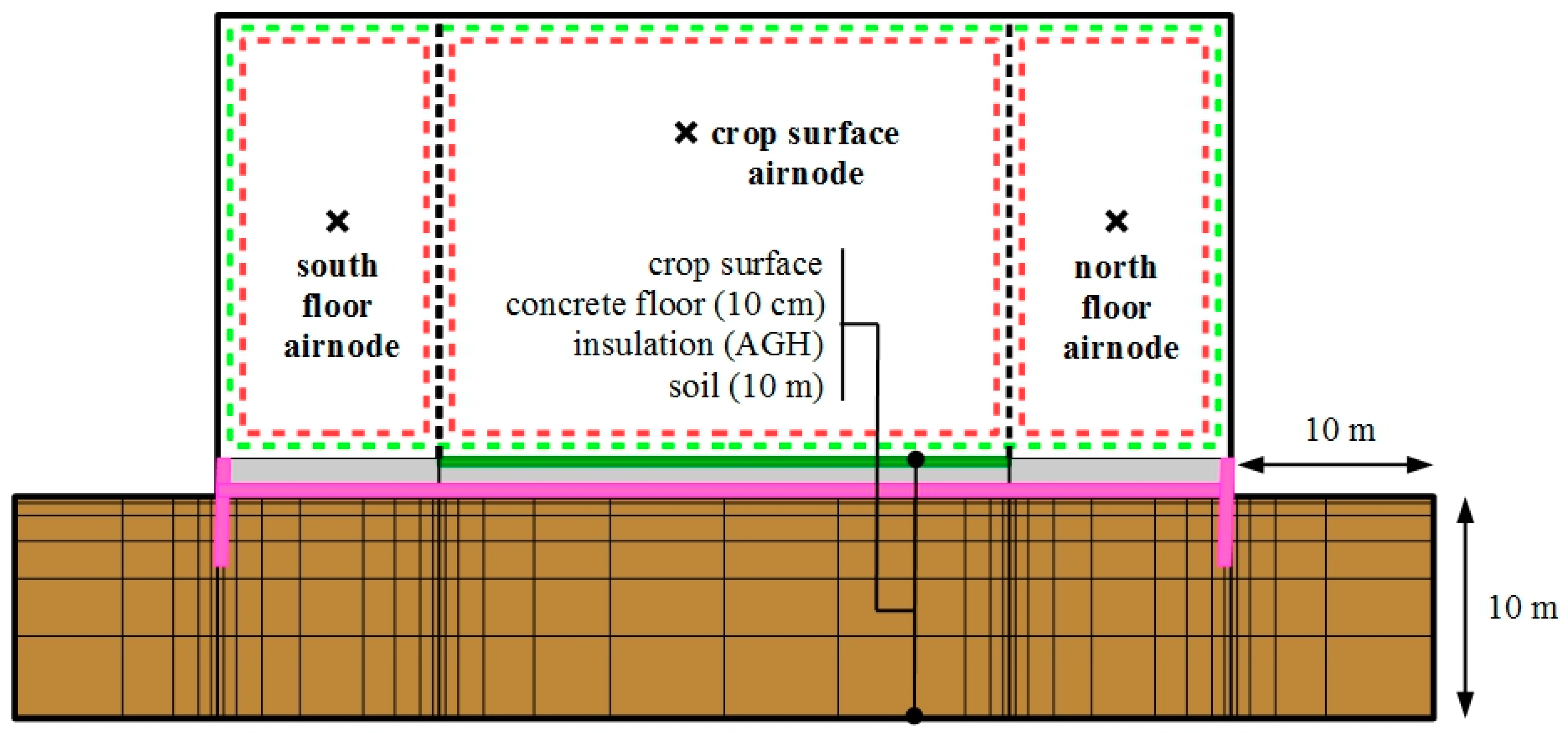
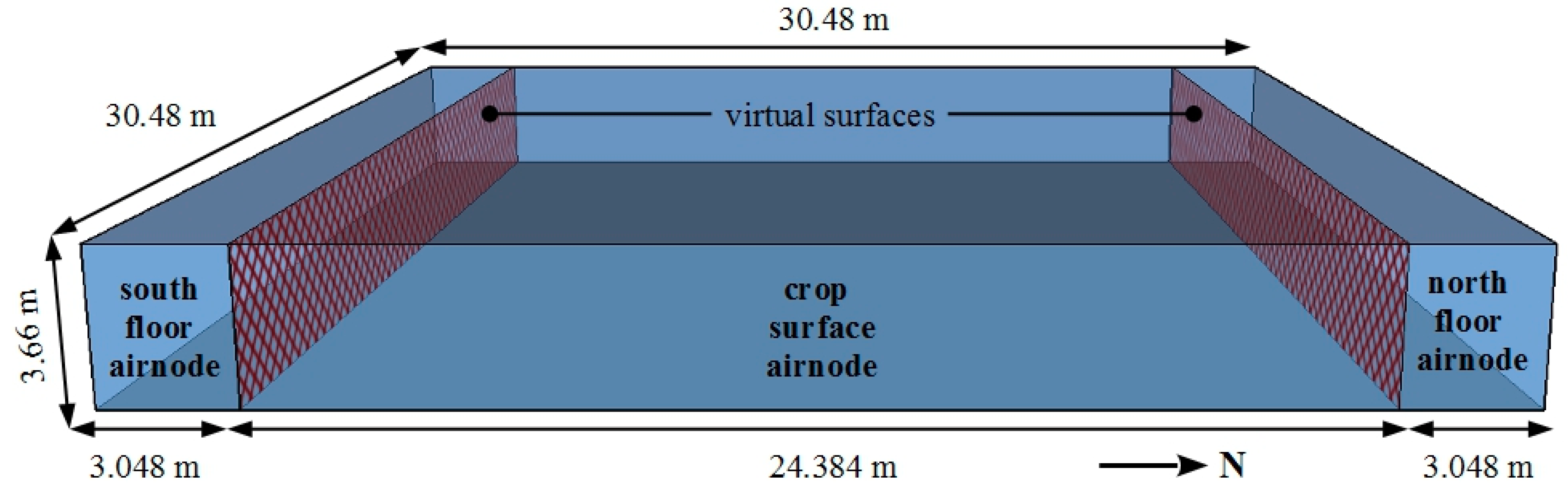
2.1. Greenhouse Characteristics

A schematic of the 929.03 m² (10,000 ft²) greenhouse considered for this study is provided in Figure 1. It has an equal length and width of 30.48 m, and a height of 3.66 m. The floor surface consists of a crop zone located between two identical floor areas (floor zone). Heating and ventilation are used to control inside humidity and temperature. The greenhouse does not utilize humidification, cooling is provided by mechanical ventilation only, and condensation is ignored in this study. The artificial lights (AL) are the only internal gain considered in the model.

2.2. Energy Analysis

TRNSYS 17.2 was selected for the transient simulation of the greenhouse climate [14]. Type 56 multizone building model was used to create the greenhouse energy model [15]. Figure 2 depicts the three most common locations for ground insulation of greenhouse: vertical along the perimeter, slanted wing, and horizontal beneath the floor. Slanted wing insulation is excluded from the analysis because of modeling limitations of the TRNSYS software (Version 17.2, Solar Energy Laboratory, Madison, WI, USA).

This study compares a base case greenhouse (BCGH) without thermal insulation to alternative designs (AGH) that consist of: (1) perimeter insulation; (2) perimeter insulation and horizontal insulation beneath the both floor zones; (3) perimeter insulation and horizontal insulation beneath both floor zones and the crop zone; and (4) perimeter insulation and horizontal insulation beneath the crop zone. Installing horizontal insulation alone is not considered because it is unlikely that it would be a viable option if perimeter insulation is not. The objective of this study is to determine whether the most cost-effective envelope design for the floor is no insulation, perimeter insulation, or a combination of perimeter and horizontal insulation. The investigation will consider two types of greenhouse floor designs: one with a concrete slab over soil (Figure 3) and another with unfinished soil (Figure 4). For the greenhouse with a ground consisting of unfinished soil, the concrete slab is replaced with a single layer of soil whose thickness is satisfactory for root development. As depicted in Figure 4, when thermal insulation is installed, it is assumed to be located beneath this layer of arable soil.

The two models which enable detailed 3D ground heat transfer in TRNSYS consist of Type 49 [16] and Type 1244 [17]. When these ground heat transfer models are selected for interaction with Type 56, each floor area must be associated with a dedicated thermal zone or airnode. Therefore, the adopted solution for enabling 3D ground heat transfer with multiple floor areas within a single zone is to separate the greenhouse into multiple airnodes. The volume associated with each airnode is dictated by the ground area which is belongs to.

The modeled greenhouse has three floor surfaces (two for the floor and one for crop zone) and therefore the single greenhouse zone is separated into three airnodes. The surface between the airnodes is defined as a “virtual” surface (shown in Figure 5), which enables unobstructed radiation heat transfer. Meanwhile, mass and energy flow between airnodes is specified by air “coupling” to maintain the well-mixed assumption (that is commonly achieved using horizontal airflow fans in greenhouses). Figure 3 and Figure 4 illustrate the three airnode greenhouse models with the discretization of the ground into control volumes. A user defined volume of soil is specified in the model so that 3D heat transfer can be calculated within this “ground zone”. Each airnode contains a certain volume of soil beneath the area that is in contact with the ground, with smaller discretization of the layers around the perimeter that are in contact with adjacent airnodes. The same concept is applied for the areas in contact with the exterior environment.

Annual and design day energy simulations of the model are performed to obtain the energy-related inputs that are needed for conducting the LCCA. The energy analysis is separated into daylight, artificial light and thermal modules. The analysis method for the daylight and artificial light modules is the same as presented by the authors in [18].

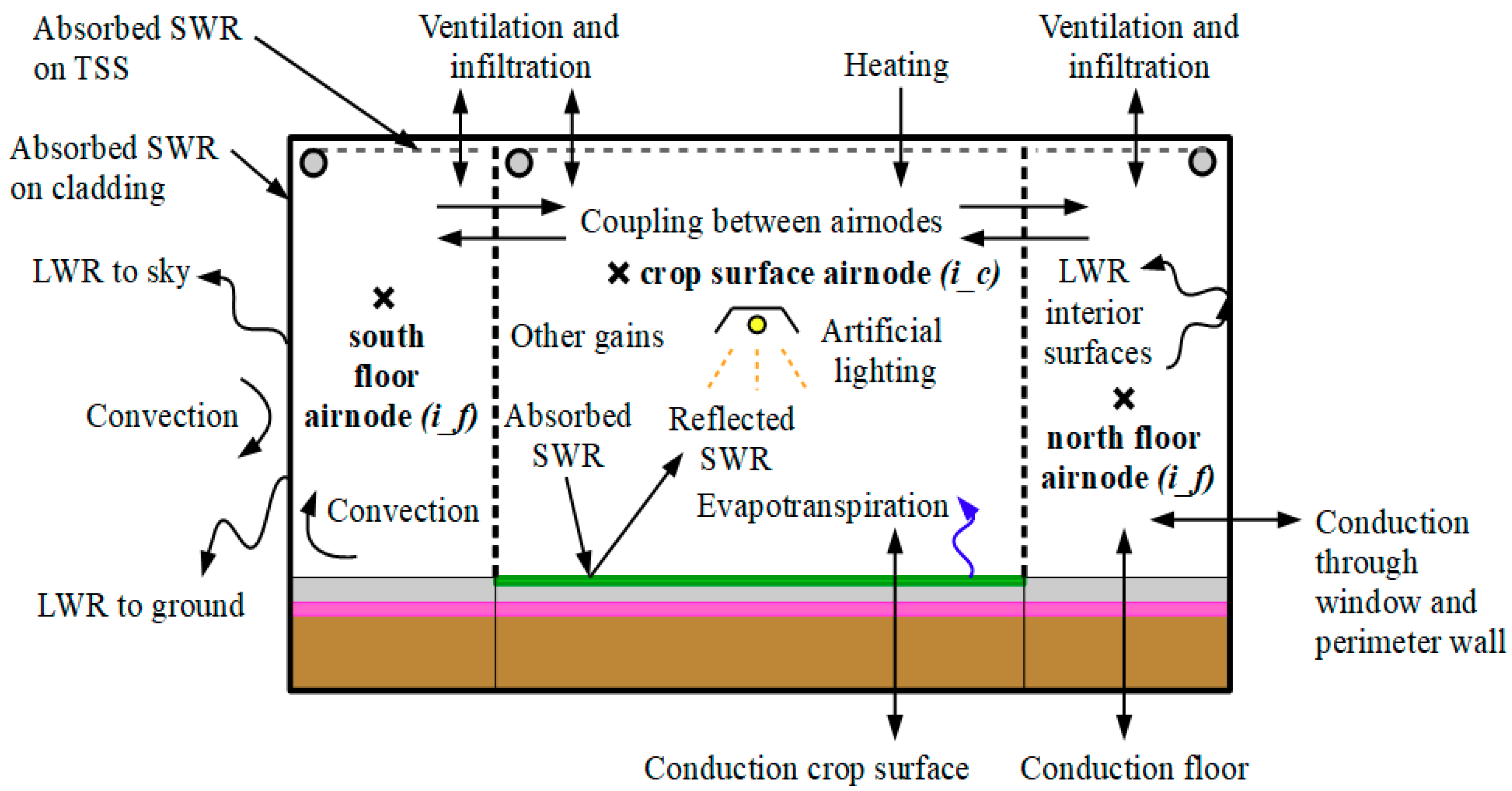
2.2.1. Thermal Module

The purpose of the thermal module is to determine the heating energy consumption and peak demand, with artificial lighting as a dynamic input. Figure 6 illustrates the major mass and energy fluxes that are considered in the three airnode greenhouse model. The energy balances are presented for the crop surface airnode that is located between the two floor airnodes (north and south sides of the greenhouse).

The mass balance for the crop surface airnode (i_c) is given by:

$$X_m·{\rho }_a·V_{i\_c}·\left(\partial {\omega }_{i\_c}/\partial t\right)=m_{vent}+m_{inf}+m_{ET}+m_{m\_cpl}$$

(1)

where:

• X_m is the moisture capacitance multiplier (dimensionless)
• ρ_a is the density of air (kg m⁻³)
• V_{i_c} is the volume of the crop zone airnode (m³)
• $\partial {\omega }_{i\_c}$ is the rate of change of the inside air humidity ratio (kg_water kg_{dry_air}⁻¹)
• $\partial t_i$ is the rate of change of time (s)
• m_vent is the mass transfer rate of water due to ventilation (kg hr⁻¹)
• m_inf is the mass transfer rate of water due to infiltration (kg hr⁻¹)
• m_ET is the mass transfer rate of water due to evapotranspiration (kg hr⁻¹)
• m_cpl is the mass transfer rate of water due air movement between the airnodes (kg hr⁻¹).

The energy balance for the crop surface airnode is written as:

$$X_{th}·{\rho }_a·c_{p\_a}·V_{i\_c}·\left(\partial T_{i\_c}/\partial t\right)=Q_{conv\_si}+Q_{vent}+Q_{inf}+Q_{TSS}+Q_{AL}+Q_{heat}+Q_{cpl}$$

(2)

where:

• X_th is the thermal capacitance multiplier (dimensionless)
• c_{p_a} is specific heat of air at constant pressure (kJ kg⁻¹ °C⁻¹)
• $\partial T_{i\_c}$ is the rate of change of the inside air temperature (°C)
• Q_{conv_si} is the energy flux due to convection (W)
• Q_vent is the energy flux due to ventilation (W)
• Q_inf is the energy flux due to infiltration (W)
• Q_TSS is the energy flux from the thermal shading screen (W)
• Q_AL is the energy flux from artificial lighting (W)
• Q_heat is the energy flux from auxiliary heating (W)
• Q_cpl is the energy flux due air movement between the airnodes (W).

The energy balance for the inside surface (si) of the cover and an opaque surface is expressed as:

$$0=Q_{cond}+Q_{conv\_si}+ Q_{swr\_si}+Q_{lwr\_si}$$

(3)

where:

• Q_cond is the energy flux due to conduction (W)
• Q_{swr_si} is the energy flux due to absorbed shortwave radiation (W)
• Q_{lwr_si} is the energy flux due to longwave radiation (W).

The energy balance for the outside surface (so) of the cover and an opaque surface is described by:

$$0=Q_{cond}+Q_{conv\_so}+Q_{swr\_so}+Q_{lwr\_sky}+Q_{lwr\_gnd}$$

(4)

where:

• Q_{conv_so} is the energy flux due to convection (W)
• Q_{swr_so} is the energy flux due to absorbed shortwave radiation (W)
• Q_{lwr_sky} is the longwave radiation energy flux to the sky (W)
• Q_{lwr_gnd} is the longwave radiation energy flux to the ground (W).

Neglecting chemical energy conversion by photosynthesis, the energy balance for the crop interior surface is defined as:

$$0=Q_{cond}+Q_{swr\_c}+Q_{swr\_c\_AL}+Q_{conv\_si}+Q_{lwr\_si}-Q_{ET}$$

(5)

where:

• Q_{swr_c_AL} is the energy flux due to absorbed shortwave radiation on the crop surface (W)
• Q_ET is the energy flux due to evapotranspiration (W).

The mass balance for each floor airnode (i_f) is given by:

$$X_m·{\rho }_a·V_{i\_f}·\left(\partial {\omega }_{i\_f}/\partial t\right)=m_{vent}+m_{inf}+m_{cpl}$$

(6)

The energy balance for each floor airnode is written as:

$$X_{th}·{\rho }_a·c_{p_a}·V_{i\_f}·\left(\partial T_{i\_f}/\partial t\right)=Q_{conv\_si}+Q_{vent}+Q_{inf}+Q_{TSS}+Q_{cpl}$$

(7)

The energy balance for the floor inside surface is expressed as:

$$0=Q_{cond}+Q_{swr\_si}+Q_{conv\_si}+Q_{lwr\_si}$$

(8)

2.2.2. Energy Modeling Key Assumptions

The details and assumptions for calculating the variables in the above energy and mass balance equations, when different than the values provided in [18], are presented below:

Weather data: A typical meteorological year weather file for Ottawa, Ontario, Canada (45.4° N, which represents mid-latitude climatic conditions) was used to run the simulations and obtain the energy performance over a one-year period. The temperature of the far-field soil is set using the Kasuda correlation which estimates the temperature of the soil at a given depth given the time of year, the soil properties, the average annual soil surface temperature, the amplitude of the annual soil surface temperature, and the day of the year at which the minimum annual surface temperature occurs [19]. Type 15 calculates the sky temperature for longwave radiation calculations [16]. A simulation timestep (Δt) of 15 min was selected. The energy model was simulated for 638 days, with the first nine months of results discarded to eliminate the initial condition transient effects. For an analysis at peak heating design conditions, no solar radiation, a wind speed of 10 m s⁻¹, exterior air relative humidity of 20%, exterior air temperature of −21.8°C, sky temperature of −52 °C, and ground temperature of 8 °C were selected [20].

Ground heat transfer: The ground surface is divided in two floor zones and one crop zone (80% of footprint). The moisture effects are not accounted for in the model. The type of crop produced is a leafy green vegetable (e.g., lettuce, kale). The crop layer is approximated as a smooth and uniform surface located directly above the concrete slab or soil surface and its thermal resistance and capacitance are ignored.

Several models with varying levels of detail exists in TRNSYS for calculating heat transfer with the ground. Type 49 and 1244 are the most detailed models because they enable 3D heat transfer to be calculated between the Type 56 multi-zone building model and the ground surface. A user defined volume of soil is considered for ground heat transfer and divided into control volumes that are assumed to be cubic in shape so there are six unique heat transfers to analyze per control volume. There are several other available methods to solve coupled 3D differential heat transfer equations using iterative methods. Type 49 uses an approximate analytical solution [16] whereas Type 1244 uses finite difference [21]. The analytical solution is timestep independent but does require an iterative solution inside the subroutine to solve the coupled differential equations.

Type 49 assumes that the ground surface is flat, that the soil has homogenous thermal properties, and that the temperature of the ground surface is not affected by the presence of the building and is instead set from long term averages. In contrast, Type 1244, does not impose the assumption of a soil surface temperature unaffected by the building and can model cases where the zone is underground. A major limitation of Type 1244 is that is cannot model perimeter insulation when the building ground level is the same as the exterior. Since perimeter insulation is a practical ground insulation technique for greenhouses, Type 49 was selected to calculate 3D heat transfer between the greenhouse and the ground.

A “map” of the soil surface was created. This map file indicates to the model whether the surface of the soil control volume is covered by one of the multi-zone building floors or whether the surface is exposed to the exterior environment. This model calculates the average surface temperature of the soil directly underneath each of the floors of the multi-zone building. These average surface temperatures are then passed to Type 56 as boundary temperature inputs for each of the floors. Based on the boundary floor temperatures provided to Type 56 by this model, Type 56 calculates the rate of energy that passes from the floors of each zone into the soil. With the soil heat transfer for each zone provided by Type 56, the thermal history of the soil field and the properties of the soil known, the temperatures of each of the control volumes of the 3D soil field can be calculated by this model. Based on the calculated soil temperatures and the zone heat flows, the average zone surface temperatures can be calculated and passed back to Type 56. This iterative methodology is then solved with the standard TRNSYS convergence algorithms.

The size of the control volumes were multiplied by a factor of two as they expanded away from the perimeter of the greenhouse airnodes. The near field/far field boundary is conductive and the temperature of the far field is set by the Kasuda correlation for the x, y and z axes. The deep ground temperature is assumed to be equal to the yearly average outside air temperature. The amplitude of the annual surface temperature profile of the soil is assumed to be equal to the maximum monthly soil surface temperature minus the average annual soil surface temperature. The soil temperature was assumed to be unaffected by the building at a distance of 10 m beneath the ground surface (in the vertical direction) and 10 m from the edge of the greenhouse (in the horizontal direction).

Coupling mass and energy transfer: Air movement is specified between the three airnodes of the air thermal zone so that they are all nearly at the same temperature (well-mixed assumption). For airflow from the crop airnode (i_c) to a floor airnode (i_f), the thermal (Q_cpl in W) and moisture (m_{m_cpl} in kg hr⁻¹) gains due to coupling are calculated from:

$$Q_{cpl}=m_{cpl}·c_{p\_a}·\left(T_{i\_c}-T_{i\_f}\right)/3.6$$

(9)

$$m_{m\_cpl}=m_{cpl}·\left({\omega }_{i\_c}-{\omega }_{i\_f}\right)$$

(10)

where:

• m_cpl is coupling mass flow of air between the airnodes (kg hr⁻¹)

The factor 3.6 serves to convert units kJ hr⁻¹ to W.

Similarly, for airflow from a floor airnode to the crop airnode, the thermal gains due to coupling are defined as:

$$Q_{cpl}=m_{cpl}·c_{p_a}·\left(T_{i\_f}-T_{i\_c}\right)/3.6$$

(11)

$$m_{m\_cpl}=m_{cpl}·\left({\omega }_{i\_f}-{\omega }_{i\_c}\right)$$

(12)

where the coupling mass flow rate is selected so that the airnode temperature become nearly identical due to mixing.

2.2.3. Values of Greenhouse Design Parameters

The values of properties for different materials and components used in the case study that are different than the values provided in [18] are given in

Table 1. Parameter values of different materials/components used in the greenhouse model.

Material/Component	Parameter	Symbol	Value	Reference
Soil	Depth of arable soil layer	Dsoil_ar	0.7 m	Assumed
	Depth of ground zone and far-field distanced	Dsoil	10 m	Assumed
	Smallest control volume size	CVmin	0.1 m	Assumed
	Specific heat	cp_soil	0.84 kJ kg−1 K−1	[15]
	Density	ρsoil	3200 kg m−3
	Thermal conductivity	ksoil	2.42 W m−1 K−1
	Emissivity	εsoil	0.9	[22]
	Solar reflectance	ρsoil	0.75	[23]
	Deep earth temperature	Tde_soil	5.9 °C	[20]
	Amplitude of surface temperature	Amp	15.3 °C
	Time shift	ts	32 d	[16]
EPS ground insulation	Thickness	lins	50 mm	Assumed
	Thermal conductivity	kins	0.036 W m−1 K−1	[24]
	Specific heat	cp_ins	1.5 kJ kg−1 K−1
	Density	ρins	20 kg m−3
	Depth of vertical perimeter insulation	Dper_ins	0.61 m	Assumed

.

2.3. Economic Analysis

The economic analysis follows the same method presented by the authors in [18]. The details of the terms presented in the net savings formula, as it applies to the case study, follows:

Change in energy cost (ΔE): The real discount rate (d in %) can be derived from:

$$d=\left(1+D\right)/\left(1+I\right)-1$$

(13)

where:

• D is the nominal discount rate (%)
• I is the inflation rate (%).

The present value of the annually recurring cost for natural gas consumed heating (PV_{E_gas} in $) is calculated by:

$$P{V}_{E\_gas}=C_{gas}·m_{gas\_yr}·\left(1+e_{gas}\right)/\left(d-e_{gas}\right)·\left[1-{\left[\left(1+e_{gas}\right)/\left(1+d\right)\right]}^n\right]$$

(14)

where:

• C_gas is the natural gas price ($ m⁻³)
• e_gas is the electricity cost escalation rate (%)
• n is the study period (yr).

Modifying the ground insulation design does not impact the indoor lighting and its associated cost. The savings in energy cost is the difference between that of the AGH and BCGH (ΔE in $) expressed as:

$$\Delta E={\left[P{V}_{E\_gas}\right]}_{BCGH}-{\left[P{V}_{E\_gas}\right]}_{AGH}$$

(15)

Change in water cost: It is assumed that no difference in water consumption occurs between the AGH and BCGH.

Change in operation, maintenance and replacement cost (O&MR): It is assumed that no difference in OM&R cost occurs between the AGH and BCGH.

Change in initial investment cost (ΔInv): The additional material and installation cost for the added rigid insulation (ΔC_ins in $) is determined as follows:

$$\Delta C_{ins}=A_{ins}·\left(C_{ins\_mat}+C_{ins\_inst}\right)$$

(16)

where:

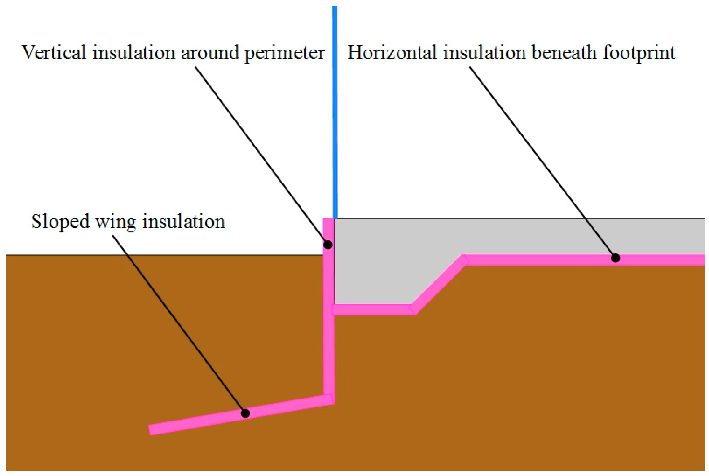
• A_ins is the area with replaced with permanent or movable insulation (m²)
• C_{ins_mat} is the material cost of insulation ($ m⁻²)
• C_{ins_inst} is the installation cost of insulation ($ m⁻²).

The AGH envelope designs reduce the peak heating energy demand and this may cause the size and associated cost of the boiler to decrease. The change in material and installation cost for the boiler (ΔC_boil in $) is computed as:

$$\Delta C_{boil}={\left[Q_{p\_heat}·\left(C_{boil\_mat}+C_{boil\_inst}\right)\right]}_{AGH}-{\left[Q_{p\_heat}·\left(C_{boil\_mat}+C_{boil\_inst}\right)\right]}_{BCGH}$$

(17)

where:

• Q_{p_heat} is the rated thermal output of the nearest commercially available boiler that can satisfy the simulated peak thermal energy demand (kW)
• C_{boil_mat} is the material cost of the boiler ($ kW⁻¹)
• C_{boil_inst} is the boiler installation cost ($ kW⁻¹).

The total additional initial investment cost (ΔInv in $) is determined as follows:

$$\Delta Inv=\Delta C_{ins}+\Delta C_{boil}$$

(18)

Change in capital replacement cost (ΔRepl): The replacement period for rigid insulation is assumed to be the same as the study period and is ignored in the LCCA. Since indoor lighting is not affected by modifying the ground envelope design, the replacement costs for artificial lighting is the same in the AGH and BCGH and can be ignored.

The cost for replacing a boiler (Repl_boil in $) is equal to:

$$Rep{l}_{boil}=Q_{p\_heat}·\left(C_{boil\_mat}+C_{boil\_lab\_repl}\right)/{\left(1+d\right)}^{P_{boil}}$$

(19)

where P_boil is the boiler lifespan (yr).

The total additional capital replacement cost (ΔRepl in $) is the difference between that of the AGH and BCGH is expressed as:

$$\Delta Repl={\left[Rep{l}_{boil}\right]}_{AGH}-{\left[Rep{l}_{boil}\right]}_{BCGH}$$

(20)

Change in residual value (ΔRes): The residual value for the boilers (Res_boil in $) is approximated by:

$$Re{s}_{boil}=Q_{p\_heat}·\left(C_{boil\_mat}\right)·\left[roundup\left(n/P_{boil},0\right)-n/P_{boil}\right]/{\left(1+d\right)}^n$$

(21)

The total residual value (ΔRes in $) is the difference between that of the AGH and BCGH given by:

$$\Delta Res={\left[Re{s}_{boil}\right]}_{AGH}-{\left[Re{s}_{boil}\right]}_{BCGH}$$

(22)

Initial investment cost (Inv): The initial investment cost of the greenhouse (Inv in $) is taken as the sum of the structure (framing, foundation, floor, covering and TSS), HVAC (ventilation and heating system) and AL components.

$$Inv=A·\left(C_{stru\_tot}+C_{HVAC\_tot}+C_{AL\_tot}\right)$$

(23)

where:

• C_{stru_tot} is the installed cost of the greenhouse structure per unit area ($ m⁻²)
• C_{HVAC_tot} is the installed cost of the HVAC system per unit area ($ m⁻²)
• C_{AL_tot} is the installed cost of the AL system per unit area ($ m⁻²).

Values of Greenhouse LCCA Parameters

The relevant cost data (in $CAD 2017) that is not presented in [18] is provided in

Table 2. Values of the cost data used in the LCCA.

Parameter	Symbol	Value	Reference
Initial investment cost of greenhouse	Inv	$712,700 (concrete floor) $655,200 (soil floor)	Calculated based on [18]
EPS insulation cost	Cins_mat	6.51 $ m−2	[25]
EPS insulation installation cost	Cins_inst	5.76 $ m−2	[25]

.

3. Results and Discussion

3.1. Portion of Heat Loss through Ground

The average heat loss pathways for the BCGH with a concrete slab in January, were determined to be: 18.6% for infiltration, 21.9% for ventilation, 37.7% from the roof, 17.8% from the walls and 4.0% from the ground. These results are from sunset to sunrise because the ground becomes a source of heat gain when sunlight exists. The portion of the envelope heat loss (walls, roof and ground) that occurred through the ground was approximately 7%. Consequently, permutations in the ground envelope design will have a small impact on the overall greenhouse energy savings.

3.2. Net Savings Achieved by the Ground Insulation Configurations

The present-value costs, residual value, NS (in $CAD 2017), and change in LCC for the AGH and BCGH are provided in

Table 3. Present-value costs, residual value, NS, and change in LCC for the greenhouse models.

Floor Type	Insulation Location and Thickness	Energy Cost	Incremental Initial Investment Cost	Capital Replacement Cost	Residual Value	NS	Change in LCC
Concrete slab	BCGH (no insulation)	$1,582,202	$0	$84,949	$25,586	-	-
	Vertical perimeter	$1,579,716	$912	$84,949	$25,586	$1575	−0.1%
	Vertical perimeter and horizontal floor zones	$1,577,112	$3192	$84,949	$25,586	$1899	−0.1%
	Vertical perimeter and horizontal floor plus crop zones	$1,577,726	$12,311	$84,949	$25,586	−$7835	0.3%
Soil floor	BCGH (no insulation)	$1,567,120	$0	$84,949	$25,586	-	-
	Vertical perimeter	$1,564,725	$912	$84,949	$25,586	$1483	−0.1%
	Vertical perimeter and horizontal floor zones	$1,560,546	$3192	$84,949	$25,586	$3382	−0.2%
	Vertical perimeter and horizontal floor plus crop zones	$1,560,371	$12,311	$84,949	$25,586	−$5562	0.2%

. The two main design alternatives for ground insulation consist of adding vertical insulation around the greenhouse perimeter and horizontal insulation beneath the floor and/or crop zones. The perimeter insulation is considered as the first design alternative because it is the most likely to provide NS. It should be noted that perimeter insulation also has the added benefit of foundation frost protection and improved crop root zone temperatures and therefore, there may be an incentive to apply it even if it does not result in NS. If NS are obtained for perimeter insulation, then the next design alternatives will be to consider horizontal insulation beneath the floor zone. If perimeter insulation does not provide NS, then subsequent designs would only consider horizontal insulation, although it is unlikely that horizontal insulation would be cost effective if perimeter insulation is not. Based on this economic result, two possibilities for subsequent envelope designs will be considered. If combined perimeter and floor zone insulation provides higher NS crop zone insulation (entire footprint). If not, the case of perimeter and crop zone insulation will be assessed. The use of ground insulation had a negligible impact on the peak energy demand for heating and therefore changes in the heating system cost are not considered.

For the concrete slab and soil floor greenhouse designs, the economic results were improved when perimeter insulation is applied (NS of $1575 and $1483, respectively and the LCC decreased by 0.1% for both). When horizontal floor insulation is added, the NS increased by 20.6% for the greenhouse with a concrete slab and 128.0% for the greenhouse with a soil floor. When horizontal crop zone insulation was added, a financial loss of $7835 (0.3% increase in LCC) was observed for the greenhouse with a concrete slab and $5562 (0.2% increase in LCC) for the greenhouse with a soil floor. Therefore, the most cost-effective design for the greenhouses with a concrete slab and soil floor is when perimeter and floor zone horizontal insulation are applied. Although this analysis provided insight into the most cost-effective greenhouse ground insulation design for Ottawa, the NS are negligible compared to the greenhouse LCC (decrease in LCC of 0.1% and 0.2% for the greenhouse with a concrete slab and soil floor, respectively).

3.3. Impact of Insulation on Energy Consumption

Table 4. Energy consumption for the greenhouse models.

Floor Type	Insulation Level	Lighting Electricity Consumption (kWh yr−1)	Natural gas Consumption for Heating (m³ yr−1)
Concrete slab	BCGH (no insulation)	114,971	61,903
	Vertical perimeter	114,971	61,690
	Vertical perimeter and horizontal floor zones	114,971	61,466
	Vertical perimeter and horizontal floor plus crop zones	114,971	61,519
Soil floor	BCGH (no insulation)	115,755	60,105
	Vertical perimeter	115,755	59,900
	Vertical perimeter and horizontal floor zones	115,755	59,541
	Vertical perimeter and horizontal floor plus crop zones	115,755	59,526

gives the annual lighting electricity use and fuel consumed for heating. The BCGH with the soil floor consumed 0.7% more electricity for lighting than the concrete floor BCGH due to the higher solar absorptance of soil compared to concrete. Meanwhile, the increased thermal energy storage in the soil caused heating energy use to decrease by 2.9%. It is interesting to note that for the concrete greenhouse, the heating energy use was lowest for the case of perimeter and floor zone insulation (natural gas use of 61,466 m³ yr⁻¹), whereas it slightly increased to 61,519 m³ yr⁻¹ when crop zone insulation was also employed. This demonstrates how, in certain cases, the use of ground insulation can be detrimental to energy conservation efforts because it reduces the potential for passive solar heating. For the designs that achieved the highest NS, heating energy was reduced by 0.6% for the greenhouse with a concrete slab and 1.0% for the soil floor. Therefore, employing ground insulation produced negligible energy savings and economic benefit for the location that was investigated. It should be noted that a single insulation thickness was selected for this study. The analysis could be repeated for different thicknesses of EPS insulation to identify the optimal level.

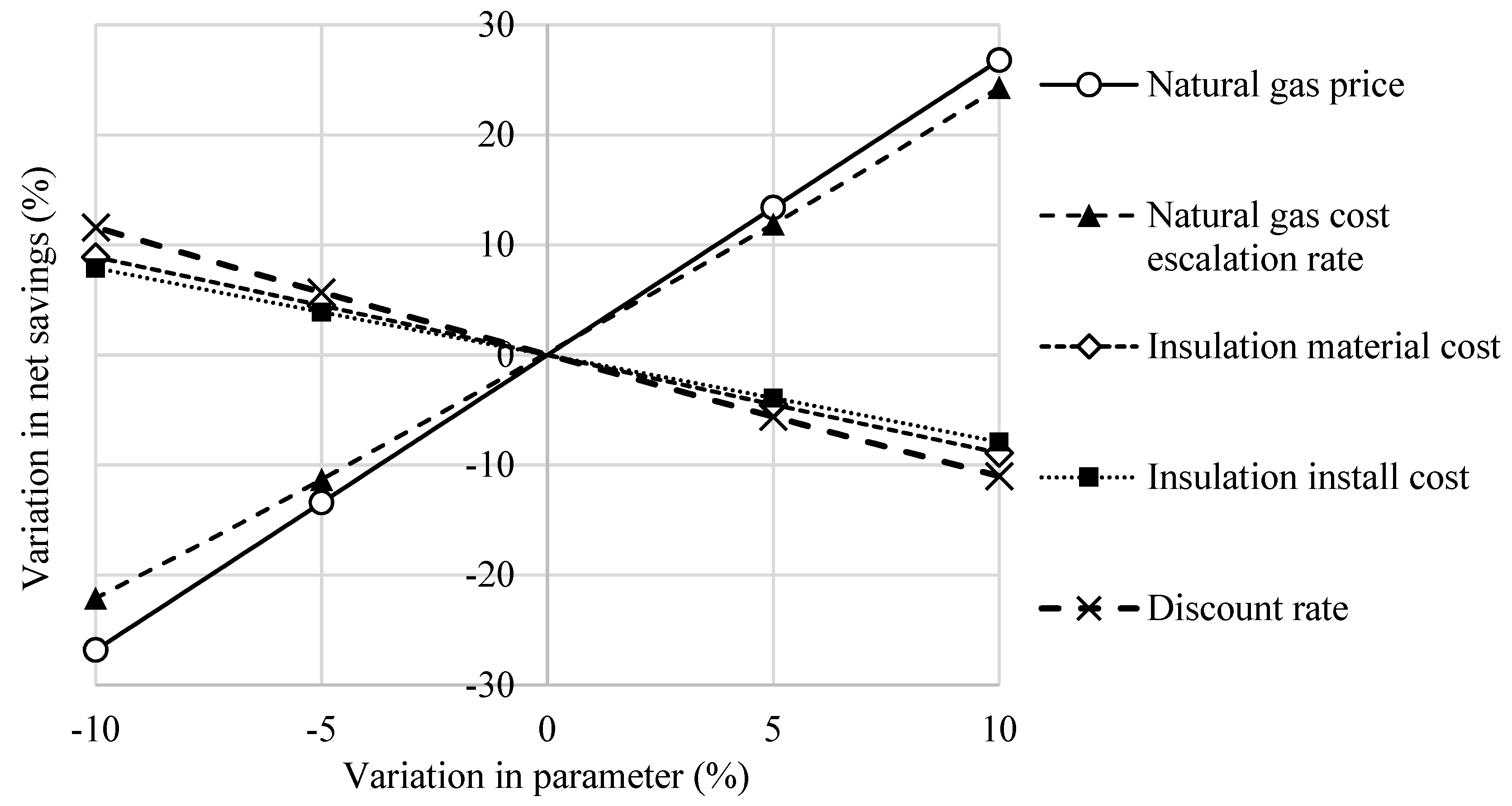
3.4. Sensitivity of Net Savings to Energy Model Input Parameter Values

The energy model input parameters to be considered are those that significantly impact energy consumption and whose value carries considerable uncertainty. In this study, the interior surface convective heat transfer coefficients for the floor and crop zones will be assessed because they may have a significant impact on predicted heating energy use and their values are not well known.

Therefore, the analysis was repeated using model parameter values that would result in higher/extreme heating energy use. An interior ground surface convective heat transfer coefficient (CHTC) value of 20 W m⁻² °C⁻¹ (representing high-mixing of greenhouse air using horizontal airflow fans) was selected for the comparison.

Table 5. Effect of ground surface CHTC for the greenhouse with a concrete slab.

Item	Insulation Level	Internal Calculation of CHTC	CHTC Increased to 20 W m−2 °C−1	% Change
Natural gas consumption for heating (m3 yr−1)	BCGH	61,903	70,359	13.7%
	50 mm vertical perimeter and horizontal floor plus crop zones	61,466	69,611	13.3%
Net savings	50 mm vertical perimeter and horizontal floor plus crop zones	$1899	$5521	190.8%

presents the results for ground surface CHTC for the greenhouse with a concrete slab. A higher CHTC increased the heating energy consumption by 13.7% for the BCGH and 13.3% for the AGH design with the highest net savings. Although its effect on heating energy use is relatively small, the net savings increased significantly (190.8%). Therefore, the inside floor surface CHTC is a modeling parameter that greatly influences the economic result. By overestimating its value, the predicted net savings could be too optimistic. Consequently, efforts should focus on accurately determining this parameter for the specific ground cover and airflow patterns that exist inside the greenhouse.

3.5. Sensitivity of Net Savings to Economic Parameter Values

It is impossible to know for certain what the price of energy, materials, labor and equipment will actually be over the next 25 years or so. To identify the critical input values in the LCCA, several parameters were individually varied by ±5 and ±10% and plotted against the resulting percent changes in net savings. When one variable is modified, all others remain at their default values. Figure 7 provides the results for the envelope design with highest net savings for the greenhouse with a concrete floor. Based on Figure 7, the critical input values (which provoke a change in NS greater than ±1% when varied by ±10%) in the LCCA include the natural gas price, natural gas cost escalation rate, the discount rate, and the insulation material and installation cost. A 10% increase in the natural gas price, natural gas cost escalation rate, discount rate, insulation material and installation cost caused the net savings to change by 26.8%, 24.3%, −11.0%, −8.9% and −7.9%, respectively. The electricity price and cost escalation does not impact net savings because the electricity consumption for lighting is not affected by design permutations of the ground envelope for a given greenhouse design. Varying the replacement cost of artificial lights did not affect the net savings because, for all cases studied, they were replaced at the maximum fixture lifespan (15 years) rather than the bulb lifespan (50,000 h).

4. Conclusions

This paper demonstrates how the combination of integrated thermal-daylight energy analysis and life cycle cost analysis can be employed to compare envelope designs for greenhouses. To the best of the author’s knowledge, it is the first time that a 3D ground heat transfer model was used to compare floor envelope designs for a greenhouse that controls light to a consistent daily integral, based on local climatic and economic conditions.

The methodology was applied to determine the most cost-effective ground insulation design for a greenhouse located in Ottawa, ON, Canada. Two types of floor designs were investigated (concrete slab and unfinished soil floor) and the insulation installation configurations were vertical around the perimeter and horizontal beneath the footprint. The portion of total heat loss that occurred through the ground was approximately 4% and permutations in ground insulation design reduced heating energy consumption by up to 1%. For both of the floor designs considered, the greenhouses produced a higher NS when insulation was applied to both the perimeter and the surface beneath the floor zone then when it was applied to the perimeter alone. Meanwhile, adding insulation beneath the crop zone was not a viable option because it increased the LCC. In all cases, the improvement in economic performance was small (NS below $4000 and reduction in life cycle under 0.2%). Therefore, a design with perimeter insulation may be the best option because it uses the least amount of material resources and provides some cost savings in addition to frost protection, reduced risk of condensation and improved thermal comfort for the crops.

The development of a 3D ground heat transfer model (that would ideally be compatible with commercially available simulation tools such as TRNSYS and EnergyPlus) which can simultaneously handle vertical perimeter insulation (for both basements and slab on grade), horizontal insulation and wing insulation would be useful for comparing all possible ground insulation configurations. Combined energy and life cycle cost analysis is valuable for determining optimal envelope designs that are capable of lowering energy consumption, improving economics and enhancing greenhouse durability.

References

1. Deru, M.; Judkoff, R.; Neymark, J. Whole-building energy simulation with a three-dimensional ground-coupled heat transfer model. ASHRAE Trans. 2002, 109, 557–565. [Google Scholar]
2. Andolsun, S. Comparison of DOE-2.1 E with EnergyPlus and TRNSYS for Ground Coupled Residential Buildings in Hot and Humid Climates Stage 3; Technical Reports; Energy Systems Laboratory: College Station, TX, USA, 2012. [Google Scholar]
3. Chen, Y. Methodology for Design and Operation of Active Building-Integrated Thermal Energy Storage Systems. Ph.D. Thesis, Concordia University, Montréal, QC, Canada, 2013. [Google Scholar]
4. Nawalany, G.; Bieda, W.; Radoń, J.; Herbut, P. Experimental study on development of thermal conditions in ground beneath a greenhouse. Energy Build 2014, 69, 103–111. [Google Scholar] [CrossRef]
5. Al-Kayssi, A.W. Spatial variability of soil temperature under greenhouse conditions. Renew. Energy 2002, 27, 453–462. [Google Scholar] [CrossRef]
6. Kittas, C.; Karamanis, M.; Katsoulas, N. Air temperature regime in a forced ventilated greenhouse with rose crop. Energy Build. 2005, 37, 807–812. [Google Scholar] [CrossRef]
7. Ghosal, M.K.; Tiwari, G.N.; Srivastava, N.S.L. Thermal modeling of a greenhouse with an integrated earth to air heat exchanger: An experimental validation. Energy Build. 2004, 36, 219–227. [Google Scholar] [CrossRef]
8. Hepbasli, A. Low exergy modelling and performance analysis of greenhouses coupled to closed earth-to-air heat exchangers. Energy Build. 2013, 64, 224–230. [Google Scholar] [CrossRef]
9. Pieters, J.G.; Deltour, J.M. Performances of greenhouses with the presence of condensation on cladding materials. J. Agric. Eng. Res. 1997, 68, 125–137. [Google Scholar] [CrossRef]
10. Gupta, M.J.; Chandra, P. Effect of greenhouse design parameters on conservation of energy for greenhouse environmental control. Energy 2002, 27, 777–794. [Google Scholar] [CrossRef]
11. Bastien, D. Methodology for Enhancing Solar Energy Utilization in Solaria and Greenhouses. Ph.D. Thesis, Concordia University, Montréal, QC, Canada, 2015. [Google Scholar]
12. Tong, G.; Christopher, D.M.; Li, B. Numerical modelling of temperature variations in a Chinese solar greenhouse. Comput. Electron. Agric. 2009, 68, 129–139. [Google Scholar] [CrossRef]
13. Nawalany, G.; Radon, J.; Bieda, W.; Sokolowski, P. Influence of Selected Factors on Heat Exchange with the Ground in a Greenhouse. Trans. ASABE 2017, 60, 479–487. [Google Scholar]
14. Klein, S.A.; Duffie, J.A.; Mitchell, J.C.; Kummer, J.P.; Thornton, J.W.; Bradley, D.E.; Kummert, M. TRNSYS 17: A Transient System Simulation Program; Solar Energy Laboratory, University of Wisconsin-Madison: Madison WI, USA, 2014. [Google Scholar]
15. TRANSSOLAR. TRNSYS 17. Volume 5. Multizone Building Modeling with Type56 and TRNBuild; Solar Energy Laboratory, University of Wisconsin-Madison: Madison WI, USA, 2005. [Google Scholar]
16. Klein, S.A.; Duffie, J.A.; Mitchell, J.C.; Kummer, J.P.; Thornton, J.W.; Bradley, D.E.; Kummert, M. TRNSYS 17. Volume 4. Mathematical Reference; Solar Energy Laboratory, University of Wisconsin-Madison: Madison WI, USA, 2014. [Google Scholar]
17. Component Libraries for the TRNSYS Simulation Environment; Thermal Energy System Specialists: Madison, WI, USA, 2012.
18. Bambara, J.; Athienitis, A.K. Energy and economic analysis for the design of greenhouses with semi-transparent photovoltaic cladding. Renew. Energy 2019, 131, 1274–1287. [Google Scholar] [CrossRef]
19. Kasuda, T.; Archenbach, P.R. Earth Temperature and Thermal Diffusivity at Selected Stations in the United States; National Bureau of Standards: Washington, DC, USA, 1965; Volume 71.
20. RETScreen. Clean Energy Project Analysis Software; Version 4; Ministry of Natural Resources: Ottawa, ON, Canada, 2013.
21. TESS Technical Support Team; Madison, WI, USA. Personnel communication, 2017.
22. Cengal, Y.A. Heat and Mass Transfer: A Practical Approach, 3rd ed.; McGraw-Hill: New York, NY, USA, 2007. [Google Scholar]
23. Reagan, J.A.; Acklam, D.M. Solar reflectivity of common building materials and its influence on the roof heat gain of typical southwestern USA residences. Energy Build. 1979, 2, 237–248. [Google Scholar] [CrossRef]
24. Yucel, K.T.; Basyigit, C.; Ozel, C. Thermal insulation properties of expanded polystyrene as construction and insulating materials. In Proceedings of the 15th Symposium in Thermophysical Properties, Boulder, CO, USA, 22–27 June 2003. [Google Scholar]
25. RSMeans Building Construction Cost Data; The Gordian Group: Rockland, MA, USA, 2017.
Figure 1. Schematic showing the modeled greenhouse.
Energies 11 03218 g001
Figure 2. Common locations for ground insulation on buildings.
Energies 11 03218 g002
Figure 3. Greenhouse model with three airnodes and discretized ground zones.
Energies 11 03218 g003
Figure 4. Same greenhouse model as Figure 3 but with a floor consisting of unfinished soil.
Energies 11 03218 g004
Figure 5. Schematic showing the two virtual surfaces that separate the three airnodes.
Energies 11 03218 g005
Figure 6. Schematic showing the mass and energy fluxes considered in the three airnode greenhouse model.
Energies 11 03218 g006
Figure 7. Sensitivity analysis for percentage change in NS given percent change in parameter—Envelope design with highest net savings for greenhouse with concrete floor.
Energies 11 03218 g007