Magnetization-Dependent Core-Loss Model in a Three-Phase Self-Excited Induction Generator

Abstract

Steady-state, transient, as well as dynamic analyses of self-excited induction generators (SEIGs) are generally well-documented. However, in most of the documented studies, core losses have been neglected or inaccurately modeled. This paper is concerned with the accurate modeling of core losses in SEIG analysis. The core loss is presented as a function related to the level of saturation. This relation is determined experimentally and integrated into a nonlinear model of the SEIG. The nonlinear model is solved using a mathematical optimization scheme to obtain the performance parameters of the SEIG. A new set of curves describing accurate behavior of the SEIG parameters is produced and presented in this paper. The computed parameters of the model are validated experimentally, and the agreement attained demonstrates the functionality and accuracy of the proposed core-loss model.

1. Introduction

Fast-depleting fossil fuels and environmental concerns have led to considerable interest in non-conventional renewable sources of energy. Wind energy has presented itself as an important pollution-free electrical energy generation alternative to conventional fuels [1,2]. Wind energy harvesting systems are typically accompanied by generators that convert the harvested motive power into usable electrical power [1,2,3]. Of several available generators, the self-excited induction generator (SEIG) has drawn considerable attention and is preferred for electromechanical energy power recovery schemes from wind. This is because of its applicability as a standalone generator that can be used in conjunction with different conventional and non-conventional energy resources. It also has some advantages over the conventional synchronous generator, such as being cost-effective, requiring less maintenance, and being brushless [4,5,6,7,8]. Due to the growing interest in renewable energy resources and isolated power systems, the SEIG is considered one of the most important electromechanical energy power conversion devices to be used with renewable energy sources.

Steady-state, transient, and dynamic analyses of SEIG have been well studied and documented [1,3,4]. The core loss analysis and modeling were totally ignored in [5,6,7,8,9,10,11,12,13]. In addition, some core-loss modeling was included for SEIG analysis in [14,15,16,17,18,19,20] by simply adopting the method used in motors, by adding a constant resistance across the magnetizing reactance in the equivalent circuit of the generator. This is acceptable in induction motor application studies, as the motor usually operates near the unsaturation region, unlike the case of the SEIG, which has to be saturated to operate normally [5,6,7,8,9]. Furthermore, any variation in speed, load, and its power factor, and/or excitation capacitor will directly influence the level of saturation, which directly affects the core loss and, hence, the other performance variables of the machine. The aim of this paper is to provide a more accurate model for the core loss in SEIGs. This is done by considering the core loss resistance as a variable function of the level of saturation in the generator. This can be extremely important, especially in the modern, well-designed SEIGs with accurate high-saturation designs. This paper derives a mathematical model for core loss as a function of saturation in the SEIG based on experimental measurements. Consequently, an accurate representation for the SEIG for advanced theoretical analysis is re-developed. The computed parameters of the model are validated experimentally, and the agreement attained demonstrates the functionality and accuracy of the proposed core-loss model.

2. Analysis

The system used to investigate SEIG is shown schematically in Figure 1. A three-phase synchronous motor was used as a prime mover during experimental tests.

The per-phase equivalent circuit of a three-phase SEIG under R-L load is shown in Figure 2. The effect of the saturation is considered for the core loss resistance, R_c, and the magnetizing reactance, X_m. To determine the values of the circuit parameters, the generator is conventionally tested under DC, locked rotor, and no load [3,4,5,6,7,8]. Values of R_s, R_r, X_s, and X_r are found from the DC and locked rotor tests. The magnetization curve of the machine, which includes the relation of R_c and X_m against air-gap voltage (or magnetization current), is obtained from a no load test (at slip = 0), as shown in Figure 3. As clearly shown, X_m and R_c are variable according to the level of saturation as it is linked with the air-gap voltage. The magnetization curve of the machine in Figure 3 is redeveloped and depicted in Figure 4a, to be used with the circuit shown in Figure 2 to yield the SEIG performance measures. As the saturation level in the generator is variable, X_m is obviously variable and R_c must also be variable. To the best of the authors’ knowledge, this fact has been ignored in all the published research concerning SEIGs [5,6,7,8,9,10,11,12,13].

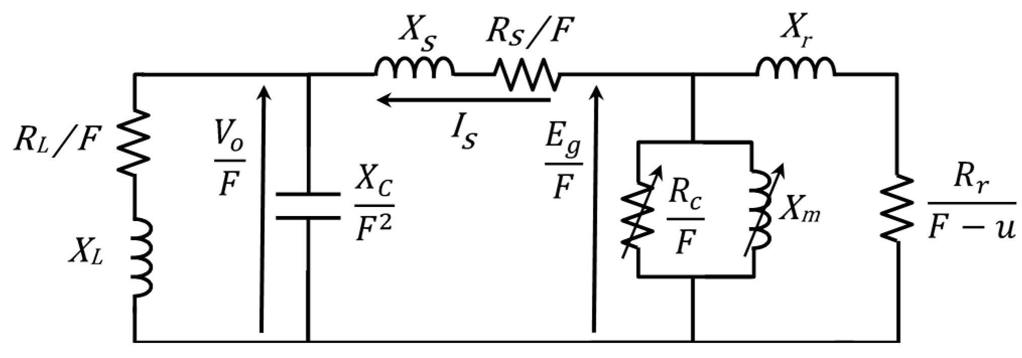
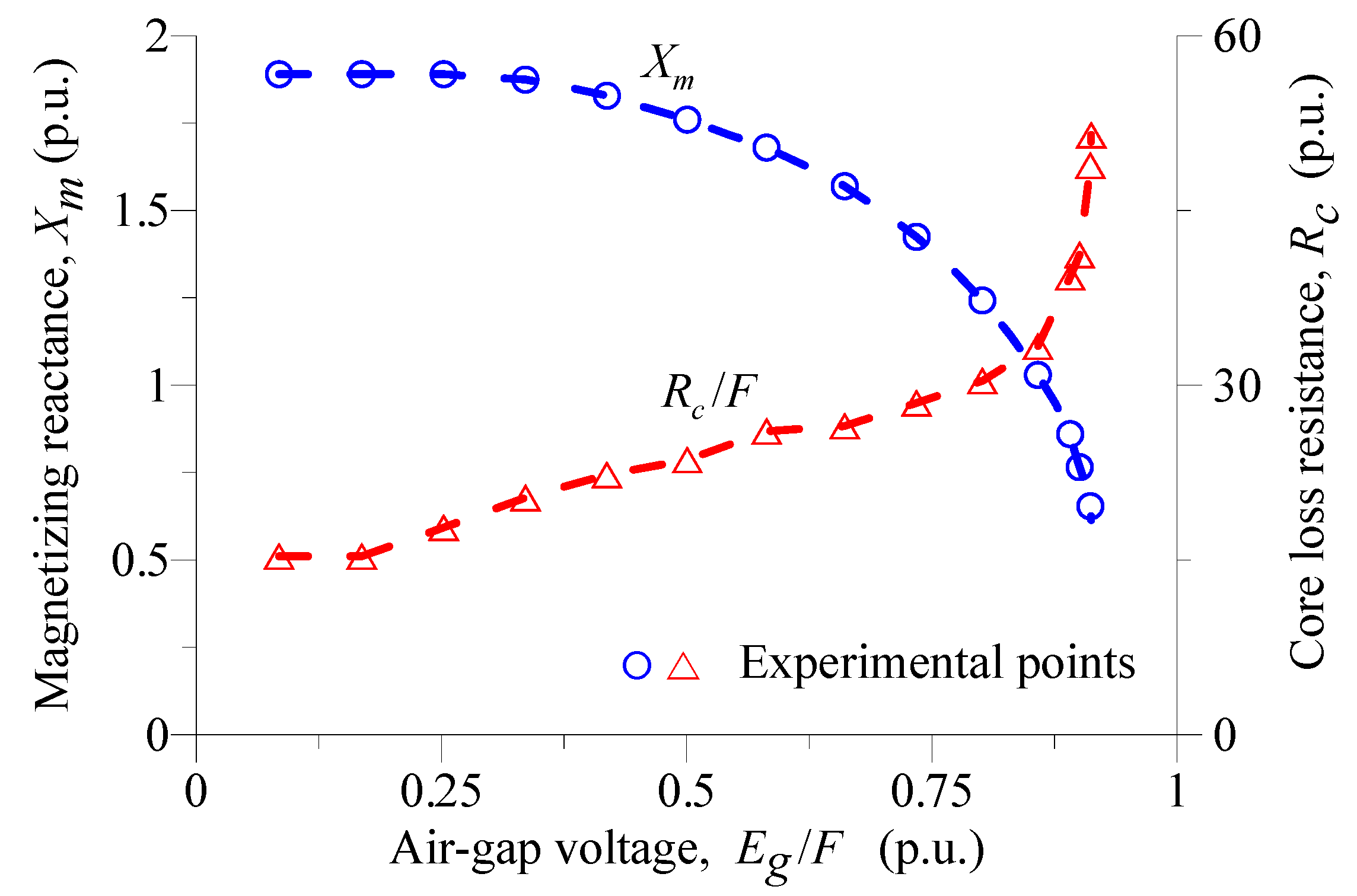
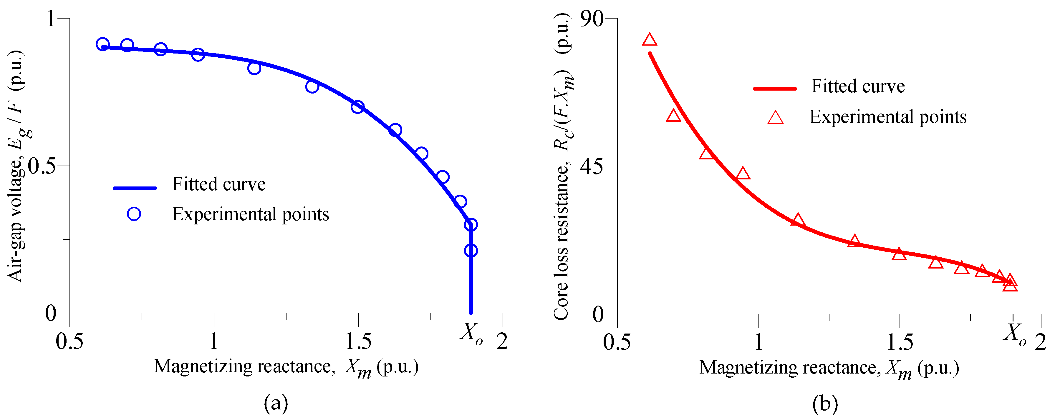
2.1. Core-Loss Modeling

To overcome the above-mentioned drawback, variable core loss can be modeled by linking the value of change rate of R_c with X_m, as shown in Figure 4b. From the experimental results in Figure 4b, the core loss, R_c, varies substantially with X_m, as illustrated by the 4th-degree polynomial fitted curve. Now, any change in load, speed or/and excitation capacitance will change the level of saturation, which, consecutively, will change the value of X_m and, hence, the value of R_c, which results in a variable core loss. For computational purposes, the curve of the air-gap voltage (E_g) versus X_m in Figure 4a is expressed either by a set of piecewise linear approximations [4,5], or by fitting the curve as a polynomial function of a suitable degree, as developed by the authors in [7].

Similarly, the relation of the core loss with X_m is also fitted as another polynomial function, as shown in Figure 4b. The fitted curves can be written as:

$$E_g/F={\displaystyle \sum _{i=0}^n{k}_i{X}_m^i}$$

(1)

$$R_c/(F·X_m)={\displaystyle \sum _{i=0}^r{m}_i{X}_m^i}$$

(2)

where k_i and m_i are the polynomial coefficients of the fitted curves that can be determined from experimental results. These two polynomial functions are as given in Appendix A. This approach does not change the characterization given in [5], yet it can solve the three unknown variables simultaneously because R_c is considered as a function of X_m.

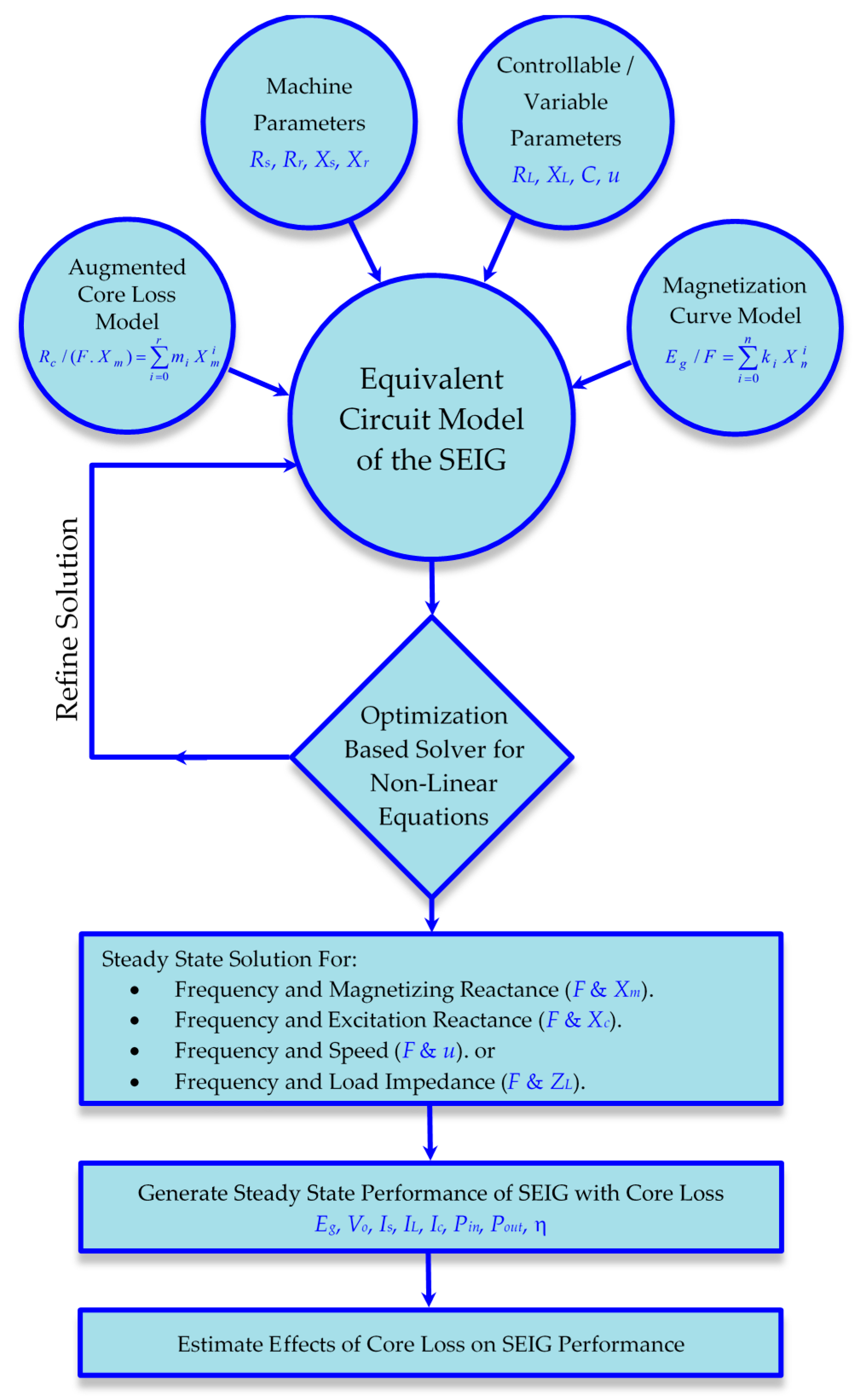
2.2. Loop-Impedance Solution

Under a steady-state condition, the following equation is applied to the circuit shown in Figure 2 [5]:

I_sZ_t = 0

(3)

where Z_t is the total impedance of the circuit across X_m and R_c branch, as given in Appendix A.

In steady state, I_s ≠ 0, which indicates that Z_t = 0, or

real(Z_t) = 0

(4)

imag(Z_t) = 0

(5)

According to the selected characterization measures, two unknowns are going to be solved, using Equations (4) and (5). These two unknowns can be (F and X_c), (F and X_m), (F and u), or (F and Z_L).

To solve the non-linear equations of (4) and (5), several schemes have been presented in recent literature. Rearranging the equations as two polynomials of a high degree in F and the other unknown is presented in [5,6]. The Newton–Raphson method is proposed to solve such a formulation in [14]. However, these methods are not appropriate to obtain the solution under the proposed varying-core-loss modeling. Alternatively, optimization-based schemes, such as that developed by the authors in [7], can be applied to solve Equations (4) and (5) under a variable core-loss condition, as explained below.

2.3. Method of Solution

The method of solution used in this paper involves the development of an optimization-based scheme that solves Equations (4) and (5) directly. This scheme simultaneously solves F and X_c or X_m, by minimizing the value of the total impedance (i.e., |Z_t| = 0). The performance of the generator described by the circuit of Figure 2 can be derived once the values of the unknowns are obtained utilizing data provided by the magnetization curve.

Figure 5 shows a block diagram of the proposed analysis which summarizes the steps that are followed to determine the value of the two unknowns. Based on these values, the performance of SEIG can be easily obtained. Figure 6 shows the flowchart of the developed program to obtain the two unknowns namely F and X_m when varying the speed of the prime mover. Similar programs were developed to solve for other unknowns such as (F and X_c), (F and u), and (F and Z_L).

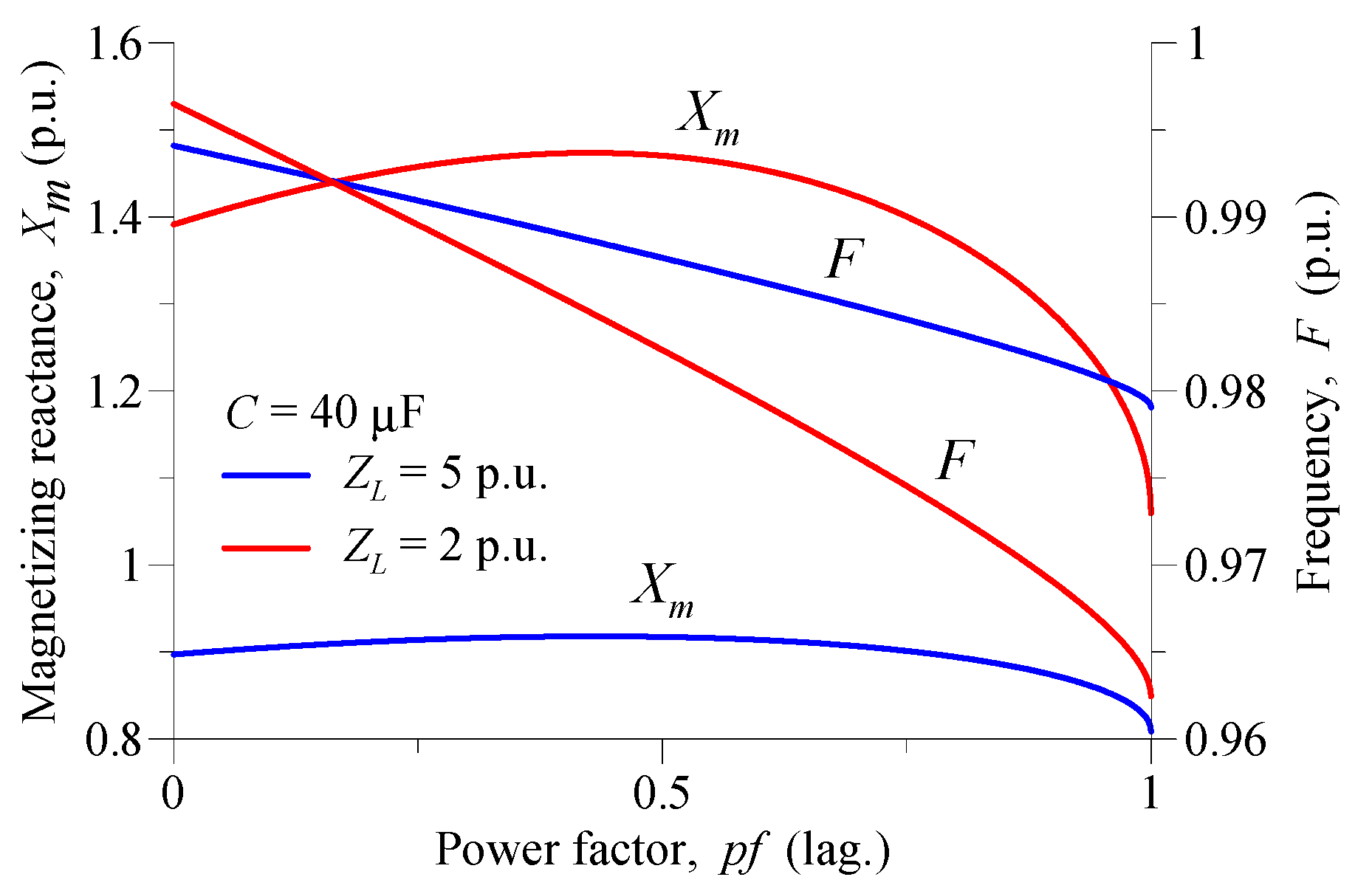
3. Results and Discussion

The SEIG performance can be controlled by controlling three parameters: excitation capacitance, speed, and load. X_m, R_c, F as well as other performance parameters of the generator vary, as these three parameters are varied. Figure 7a,b show the variations of X_m, R_c, and V_o, I_s versus the excitation capacitor, respectively, under different loading conditions. Results confirm the reliability, accuracy, and feasibility of the proposed core modeling. In Figure 7a, X_m decreases to a minimum as C is being increased and then starts increasing. R_c on the other hand increases and decreases independently from X_m. In Figure 7b, V_o changes in a concave manner, whereas I_s increases and then decreases. When X_m is greater than X_o, the machine does not generate voltage. Figure 7b is plotted for a case when the machine is generating voltage (i.e., when X_m is less than or equal to X_o) [5,6,7,8].

Figure 8 is a plot of the variations of the minimum excitation capacitor (C_min) and F versus power factor (pf) at different loads. In this case, X_m is kept constant at a value equal to X_o, and speed (u) is fixed at 1 p.u. C_min is higher for lower loads and stays nearly constant at lower pfs. When pf increases to a certain value, C_min begins to decrease. F is higher for higher loads, but decreases in very small amounts as the pf increases. Figure 9 shows the variations of X_m and F against pf with C fixed at 40 µF. It can be seen that X_m is larger for smaller loads. In addition, F is decreasing at smaller amounts as pf increases, and it decreases more for smaller loads.

Figure 10 shows the behavior of V_o, and I_s as pf is being varied at a speed of 1 p.u. while C is fixed at 40 µF. At higher loads, V_o is almost constant, and it is obvious that it is higher when X_m is lower by comparing Figure 9 and Figure 10.

Figure 11 shows the variations of X_m and R_c against speed (Figure 11a) with C fixed at 30 µF for different loads, as well as V_o and I_s against speed (Figure 11b), at the same value of C. As stated above, the machine will not generate voltage for values of X_m above X_o. It is clear from this figure that R_c varies as the speed changes which agrees with the measured results depicted in Figure 3. The assumption in many documented research publications is that it remains constant [16,17,20].

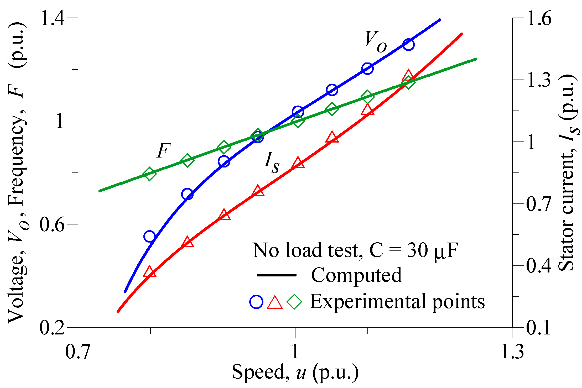
4. Experimental Verification

4.1. Setup

The machine investigated above was tested experimentally under different conditions. The experimental setup used is shown in Figure 12. A variable DC power supply was used to control the speed of the DC motor as a prime mover of the SEIG. A capacitor bank was utilized to excite the machine to operate as a generator. A computerized measurement unit (model CEM-U/Elettronica Veneta) was used to measure the electrical and mechanical quantities such as current, voltage, power, frequency, power factor, and speed. In some of these tests, a synchronous motor was used to obtain an accurate fixed speed at 1 p.u. to acquire the measurement shown in Figure 13 as well as the no load test with a slip = 0 which is used to obtain the machine parameters.

4.2. Performance Measurements

Figure 13 shows the variations of the terminal voltage, V_o, and stator current, I_s, against excitation capacitor. Figure 14 shows the variations of terminal voltage, frequency, and stator current against generator speed. Figure 14 is repeated in Figure 15 but under different excitation capacitor values. From these figures, V_o and I_s increase as C, or speed, increases. Frequency also increases, as expected, as speed increases. These figures show the superiority and accuracy of the modeling presented, as can be seen from the perfect correlation between computed and experimental results.

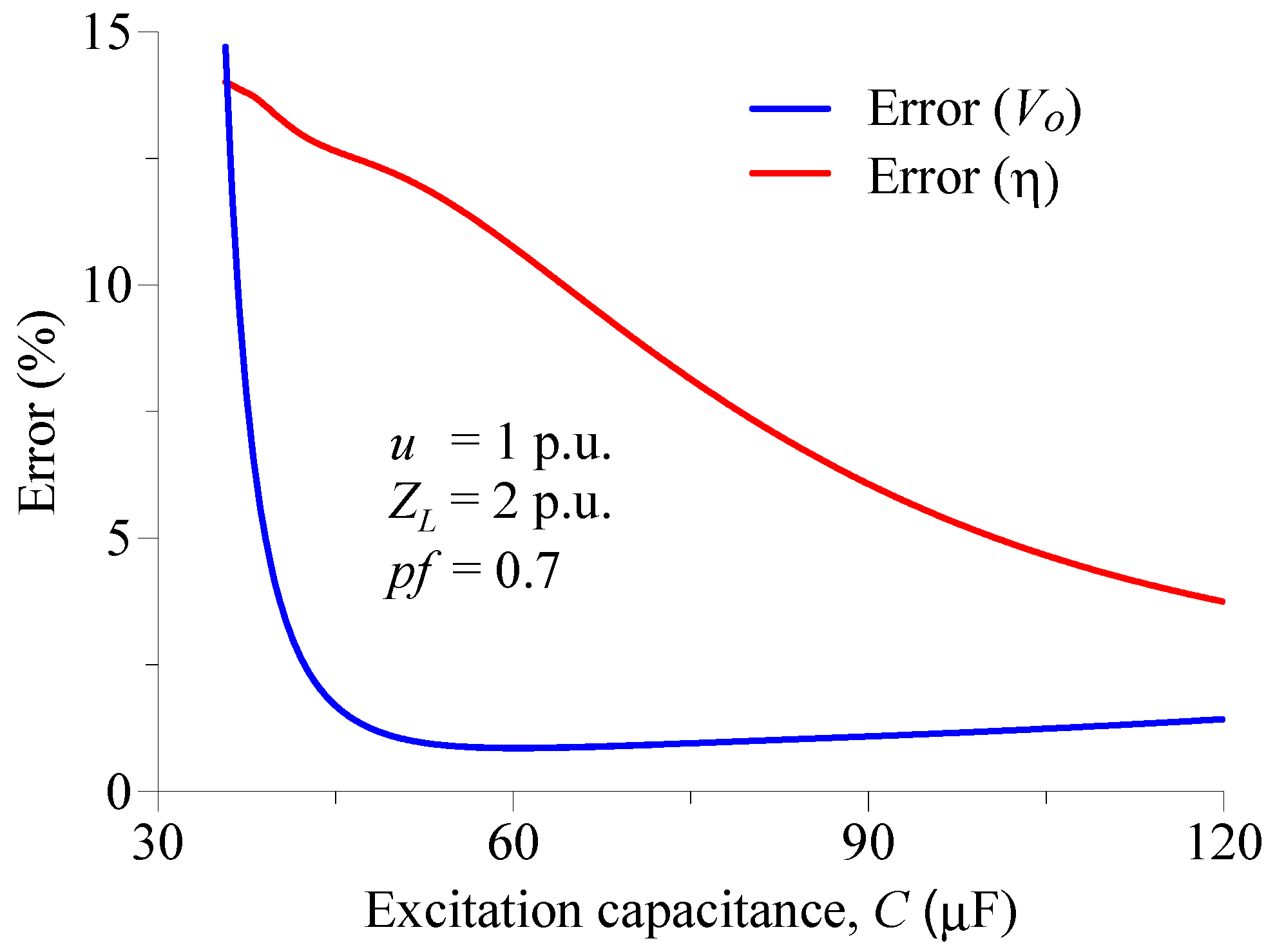
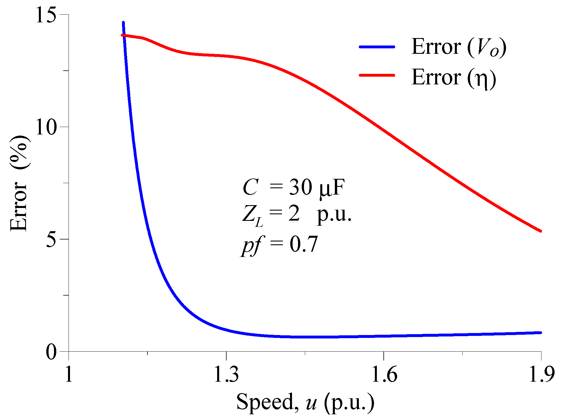
5. Influence of Core Loss

The value of the error that results from ignoring accurate core-loss modeling on the performance of the generator is studied in this section. The error is computed between the values under the presented core-loss modeling and a fixed value of R_c.

The variation of the error in the values of terminal voltage (V_o) and efficiency (η) are analyzed under different conditions for the generator under study and are shown in Figure 16, Figure 17 and Figure 18. Figure 16 shows the error variation versus excitation capacitance under fixed load and speed, while Figure 17 shows the error variation versus speed under fixed load and excitation capacitance. It can be deduced from Figure 16 and Figure 17 that the error in the value of V_o is relatively high for low C and u values, and then this error rapidly decreases as C, or u increase before it reaches an almost constant low value. On the other hand, the efficiency error variation is relatively high even at high values of C, or u.

The error variation versus load impedance, under fixed speed and excitation capacitance, is shown in Figure 18. The figure shows that the error of V_o is relatively high at low impedance values and then it rapidly decreases as the load impedance increases before it reaches a nearly constant low value. On the other hand, the efficiency error variation increases with a high percentage as the load increases.

6. Conclusions

This paper presents an accurate modeling scheme of core losses in SEIG analysis, which has been neglected in most of the documented literature. In this work, the resistance of the core loss in the equivalent circuit of the generator is derived as a function of the saturation level in the generator magnetic circuit. An optimization scheme is used to solve the derived nonlinear equations by simultaneously computing the values of F and X_c or X_m by minimizing the total impedance. Accordingly, the performance curves are computed for the machine as shown in Figure 9, Figure 10 and Figure 11. Experimental verifications were carried out to compare theoretical results with measurements. Perfect agreement between the analytical and the experimental results confirms the feasibility and accuracy as well as the functionality of the modeling presented. It has been found that representing core loss with a fixed resistance causes an error between (2–12)% in computing terminal voltage while it reaches between (15–40)% in the value of the efficiency.

References

1. Boldea, I. Variable Speed Generators, 2nd ed.; CRC Press: Boca Raton, FL, USA, 2015; ISBN 1498723578. [Google Scholar]
2. International Renewable Energy Agency (IRENA). Renewable Capacity Statistics 2017. Available online: http://www.irena.org/publications/2017/Mar/Renewable-Capacity-Statistics-2017 (accessed on 26 February 2018).
3. Musgrove, P. Wind Power, 1st ed.; Cambridge University Press: Cambridge, UK, 2010; ISBN 0521762383. [Google Scholar]
4. Singh, G.K. Self-excited induction generator research—a survey. Electr. Power Syst. Res. 2014, 69, 107–114. [Google Scholar] [CrossRef]
5. Al Jabri, A.K.; Alolah, A.I. Limits on the performance of the three-phase self-excited induction generators. IEEE Trans. Energy Convers. 1990, EC-5, 350–356. [Google Scholar] [CrossRef]
6. Al Jabri, A.K.; Alolah, A.I. Capacitance requirement for isolated self-excited induction generator. IEEE Proc. B-Electr. Power Appl. 1990, 137, 154–159. [Google Scholar] [CrossRef]
7. Alolah, A.I.; Alkanhal, M.A. Optimization-based steady state analysis of three phase self-excited induction generator. IEEE Trans. Energy Convers. 2000, EC-15, 61–65. [Google Scholar] [CrossRef]
8. Alnasir, Z.; Kazerani, M. An analytical literature review of stand-alone wind energy conversion systems from generator viewpoint. Renew. Sustain. Energy Rev. 2013, 28, 597–615. [Google Scholar] [CrossRef]
9. Sam, K.N.; Kumaresan, N.; Gounden, N.A.; Katyal, R. Analysis and Control of Wind-Driven Stand-Alone Doubly-Fed Induction Generator with Reactive Power Support from Stator and Rotor Side. Wind Eng. 2015, 39, 97–112. [Google Scholar] [CrossRef]
10. Kheldoun, A.; Refoufi, L.; Khodja, D.E. Analysis of the self-excited induction generator steady state performance using a new efficient algorithm. Electr. Power Syst. Res. 2012, 86, 61–67. [Google Scholar] [CrossRef]
11. Nigim, K.; Salama, M.; Kazerani, M. Identifying machine parameters influencing the operation of the self-excited induction generator. Electr. Power Syst. Res. 2004, 69, 123–128. [Google Scholar] [CrossRef]
12. Wang, L.; Lee, C.H. A novel analysis on the performance of an isolated self-excited induction generator. IEEE Trans. Energy Convers. 1997, EC-12, 109–117. [Google Scholar] [CrossRef]
13. Kersting, W.H.; Phillips, W.H. Phase Frame Analysis of the Effects of Voltage Unbalance on Induction Machines. IEEE Trans. Ind. Appl. 1997, IA-33, 415–420. [Google Scholar] [CrossRef]
14. Malik, N.H.; Haque, S.E. Steady State Analysis and Performance of an Isolated Self-Excited Induction Generator. IEEE Trans. Energy Convers. 1986, EC-1, 134–140. [Google Scholar] [CrossRef]
15. Sharma, A.; Kaur, G. Assessment of Capacitance for Self-Excited Induction Generator in Sustaining Constant Air-Gap Voltage under Variable Speed and Load. Energies 2018, 11, 2509. [Google Scholar] [CrossRef]
16. Hashemnia, M.; Kashiha, A. A Novel Method for Steady State Analysis of the Three Phase SEIG Taking Core Loss into Account. In Proceedings of the 4th Iranian Conference on Electrical and Electronics Engineering (ICEEE2012), Gonabad, Iran, 28–30 August 2012. [Google Scholar]
17. Farrag, M.E.; Putrus, G.A. Analysis of the Dynamic Performance of Self-Excited Induction Generators Employed in Renewable Energy Generation. Energies 2014, 7, 278–294. [Google Scholar] [CrossRef] [Green Version]
18. Arjun, M.; Rao, K.U.; Raju, A.B. A Novel Simplified Approach for Evaluation of Performance Characteristics of SEIG. In Proceedings of the 2014 International Conference on Advances in Energy Conversion Technologies (ICAECT), Manipal, India, 23–25 January 2014. [Google Scholar]
19. Selmi, M.; Rehaoulia, H. Effect of the Core Loss Resistance on the Steady State Performances of SEIG. In Proceedings of the International Conference on Control, Engineering & Information Technology (CEIT’2014), Sousse, Tunisia, 22–25 March 2014. [Google Scholar]
20. Haque, M.H. A Novel Method of Evaluating Performance Characteristics of a Self-Excited Induction Generator. IEEE Trans. Energy Convers. 2009, EC-24, 358–365. [Google Scholar] [CrossRef]
Figure 1. Schematic diagram of the system under study.
Energies 11 03228 g001
Figure 2. Per-phase equivalent circuit of the induction generator under the proposed core-loss model.
Energies 11 03228 g002
Figure 3. Variation of magnetizing reactance Xm and core loss resistance Rc/F versus air-gap voltage Eg/F in the machine under study.
Energies 11 03228 g003
Figure 4. Variation of air-gap voltage and core loss versus magnetizing reactance Xm: (a) Air-gap voltage Eg/F (b) Core loss resistance Rc/(F Xm).
Energies 11 03228 g004
Figure 5. Block diagram of the developed model.
Energies 11 03228 g005
Figure 6. Flowchart of the developed optimization program to obtain the performance of the self-excited induction generator (SEIG).
Energies 11 03228 g006
Figure 7. Variation versus excitation capacitance C for different loads at fixed speed (u = 1.0 p.u.): (a) Magnetizing reactance Xm and core loss resistance Rc (b) Terminal voltage Vo and Stator current Is.
Energies 11 03228 g007
Figure 8. Variation of minimum excitation capacitance Cmin and frequency F versus power factor pf for different loads at fixed speed (u = 1.0 p.u.).
Energies 11 03228 g008
Figure 9. Variation of magnetizing reactance Xm and frequency F versus power factor pf for different loads at fixed speed (u = 1.0 p.u.).
Energies 11 03228 g009
Figure 10. Terminal voltage Vo and Stator current Is versus power factor pf for different loads at fixed speed (u = 1.0 p.u.).
Energies 11 03228 g010
Figure 11. Variation versus speed for different loads at capacitance C = 30 µF: (a) Magnetizing reactance Xm and core loss resistance Rc (b) Terminal voltage Vo and stator current Is.
Energies 11 03228 g011
Figure 12. Experimental setup for SEIG testing.
Energies 11 03228 g012
Figure 13. Terminal voltage Vo and stator current Is versus excitation capacitance C under no load when speed (u) = 1 p.u.
Energies 11 03228 g013
Figure 14. Variation of terminal voltage Vo, stator current Is, and frequency F versus speed under no load.
Energies 11 03228 g014
Figure 15. Terminal voltage Vo, and stator current Is versus speed under no load.
Energies 11 03228 g015
Figure 16. Error variation of terminal voltage Vo and efficiency η versus excitation capacitance C.
Energies 11 03228 g016
Figure 17. Error variation of terminal voltage Vo and efficiency η versus speed u.
Energies 11 03228 g017
Figure 18. Error variation of terminal voltage Vo and efficiency η versus load impedance |ZL|.
Energies 11 03228 g018