Scaling Criteria for Axial Piston Machines Based on Thermo-Elastohydrodynamic Effects in the Tribological Interfaces

Abstract
:1. Introduction
2. Scaling of Swashplate-Type Axial Piston Machines
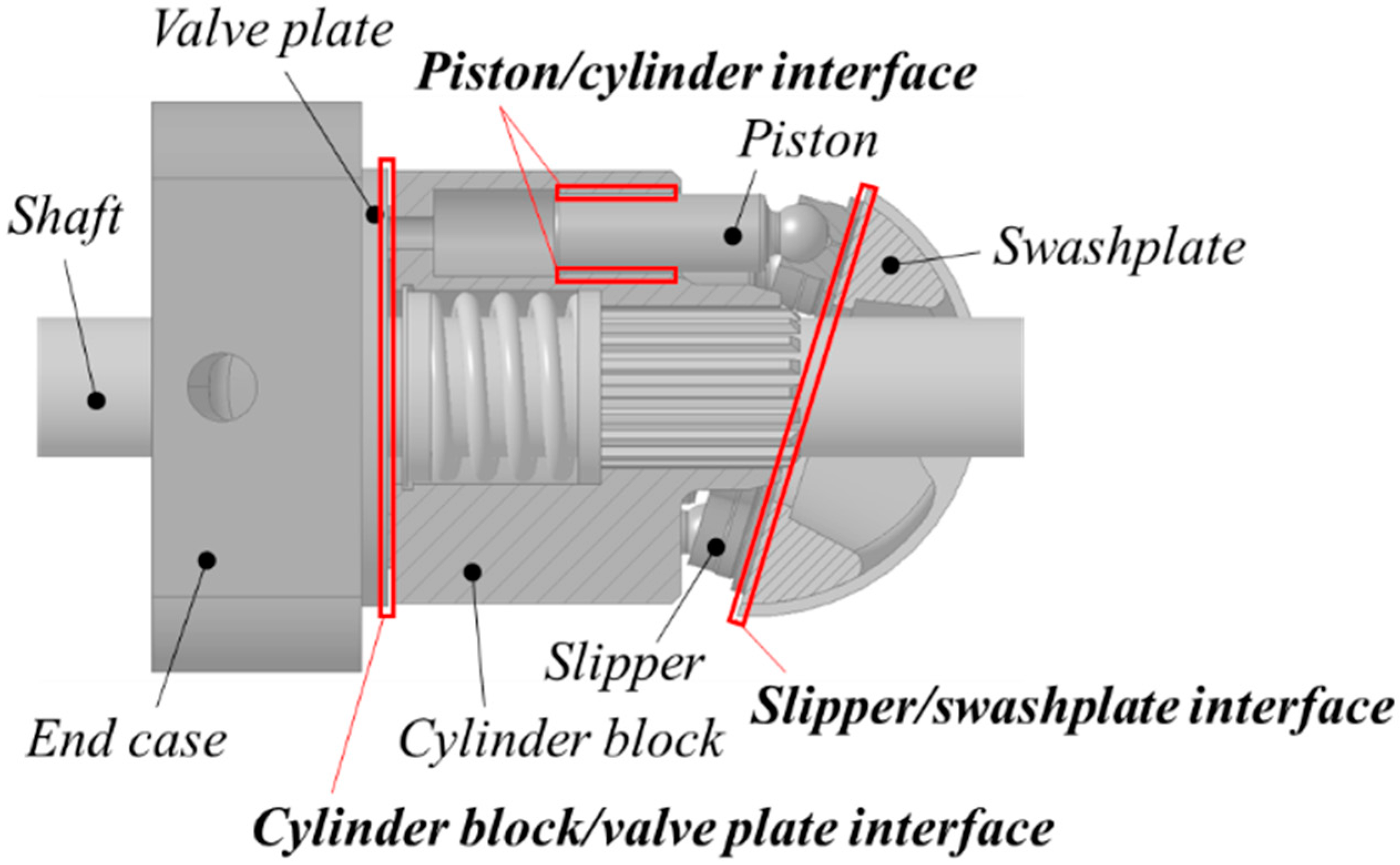
Scaling of Lubricating Interfaces in Swashplate-Type Axial Piston Machines
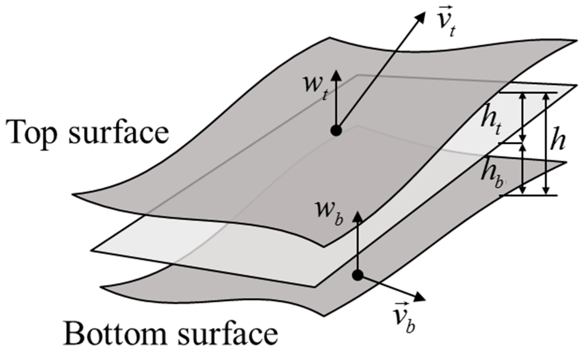
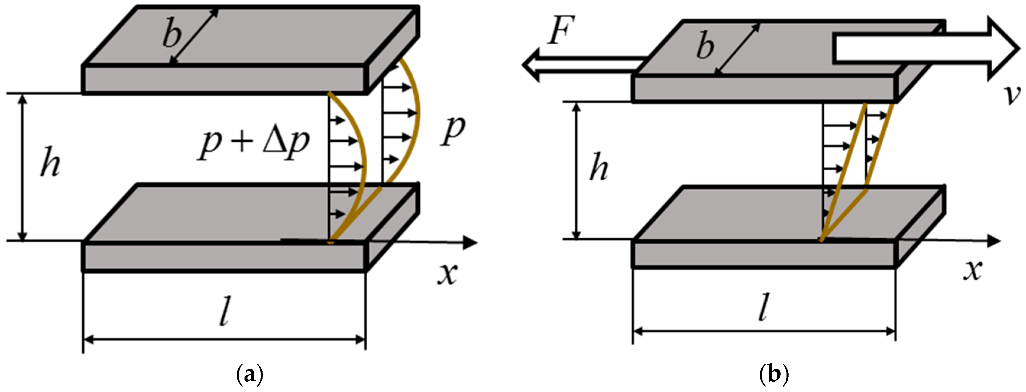
- The pressure difference across the gap pushes the fluid through the interface, generating fluid shear and energy dissipation. In this way, the energy dissipation has a positive correlation with gap height, as well as with the gap flow rate.
- The relative motion of the solid boundaries of the lubricating gap causes the fluid to shear, and dissipates energy into heat. In this way, the energy dissipation has a negative correlation with gap height.
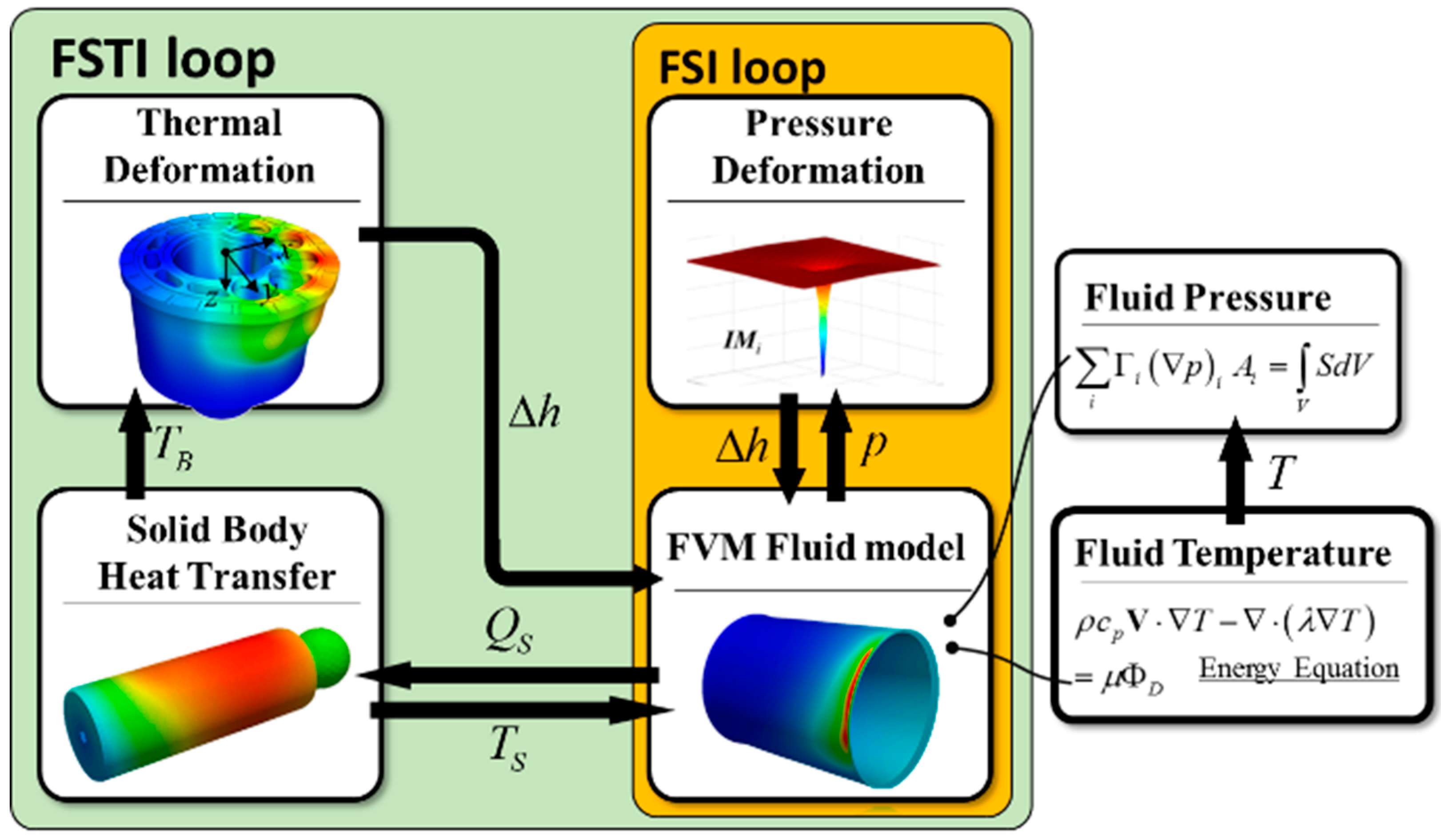
3. Fluid–Structure–Thermal Interaction Model
4. Size-Dependence of Physical Phenomena in Tribological Interfaces
4.1. Linear Scaling Method (Conventional Approach)
4.2. Analysis of the Governing Equations Describing the Fundamental Physical Phenomena in Scaled Tribological Interfaces
4.2.1. Fluid Pressure Distribution
4.2.2. Solid Body Elastic Deformation
4.2.3. Multi-Domain Heat Transfer
5. Findings and Scaling Guides
- Pressure distribution and heat transfer in both the fluid domain and the solid domain are the only contributions to the size-dependence of the axial piston machine’s lubricating interface performance.
- As long as the pressure distribution and temperature distribution are proportionally scaled, the deformation due to the pressure and thermal load stays constant, and therefore does not contribute to the size-dependence of the lubricating interface performance.
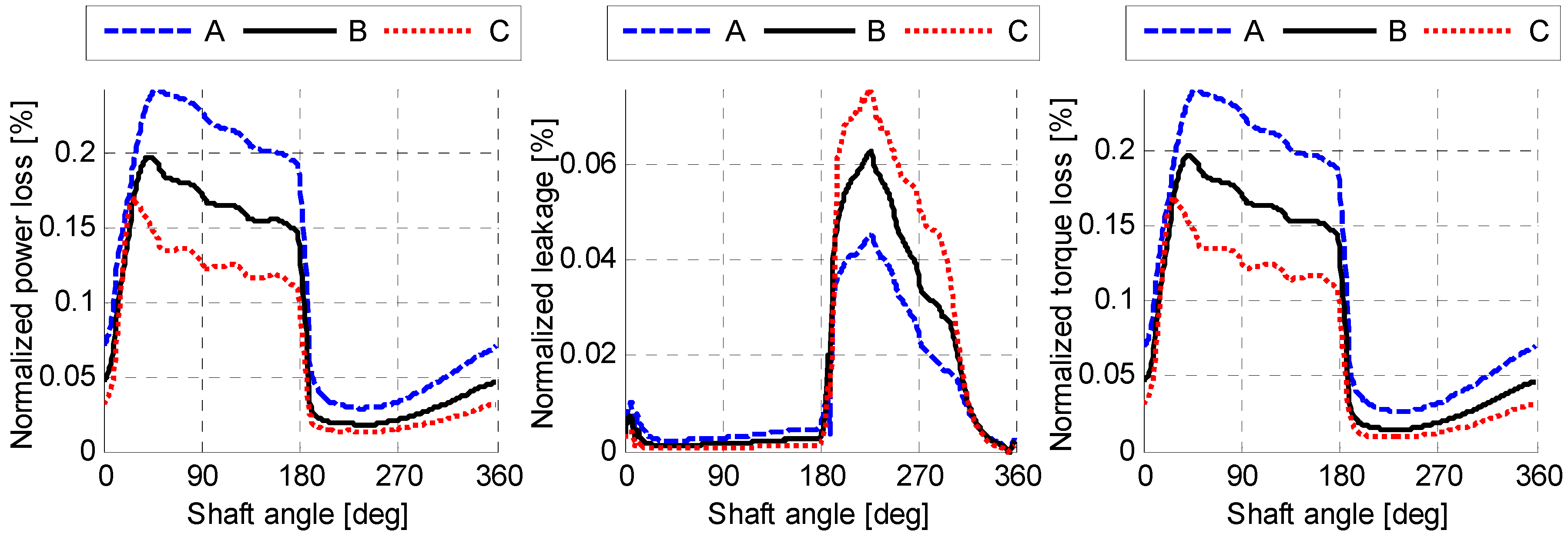
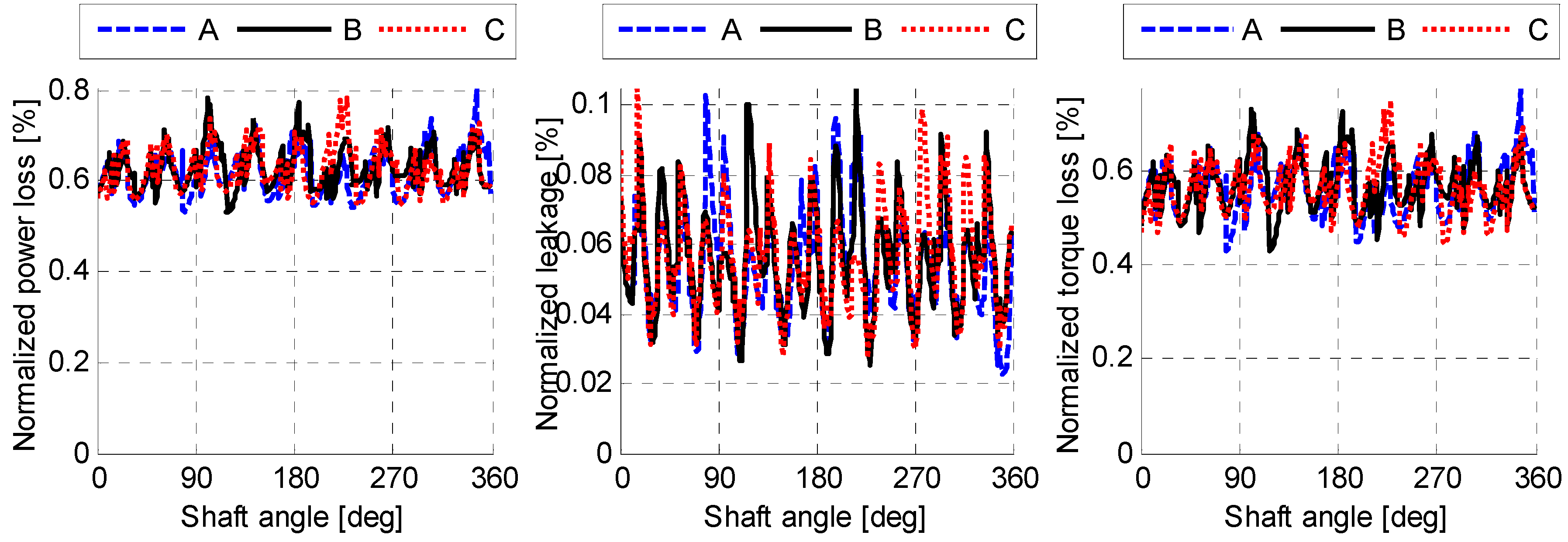
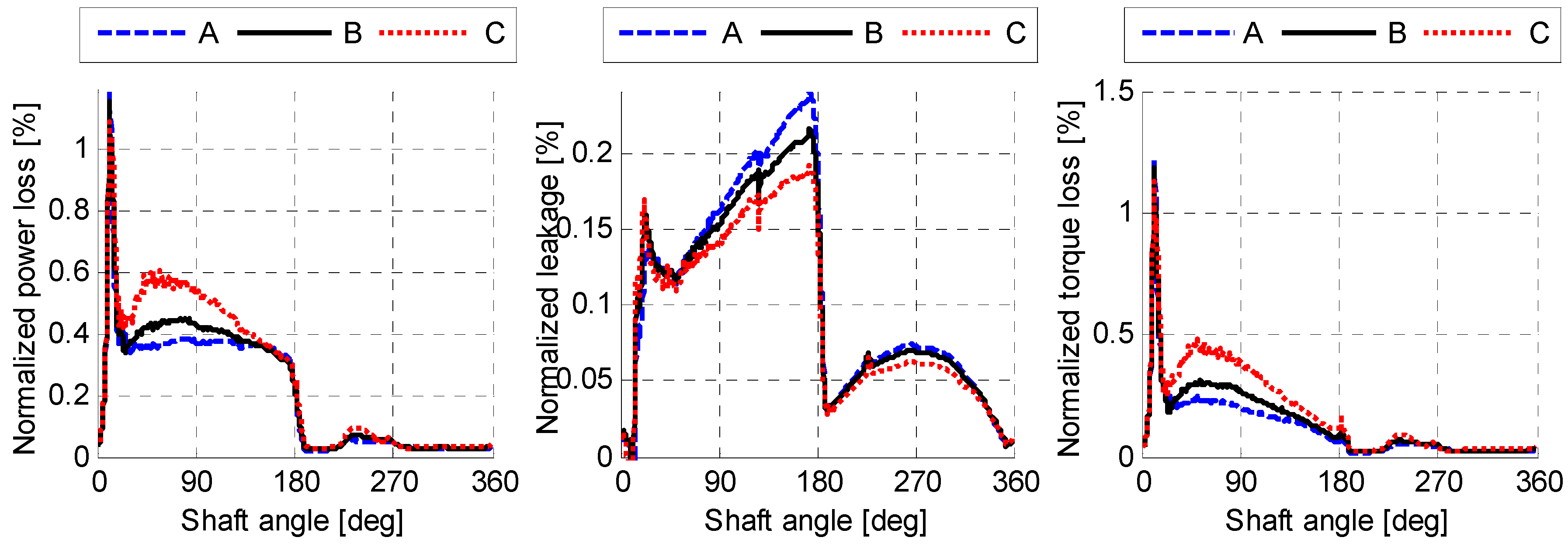
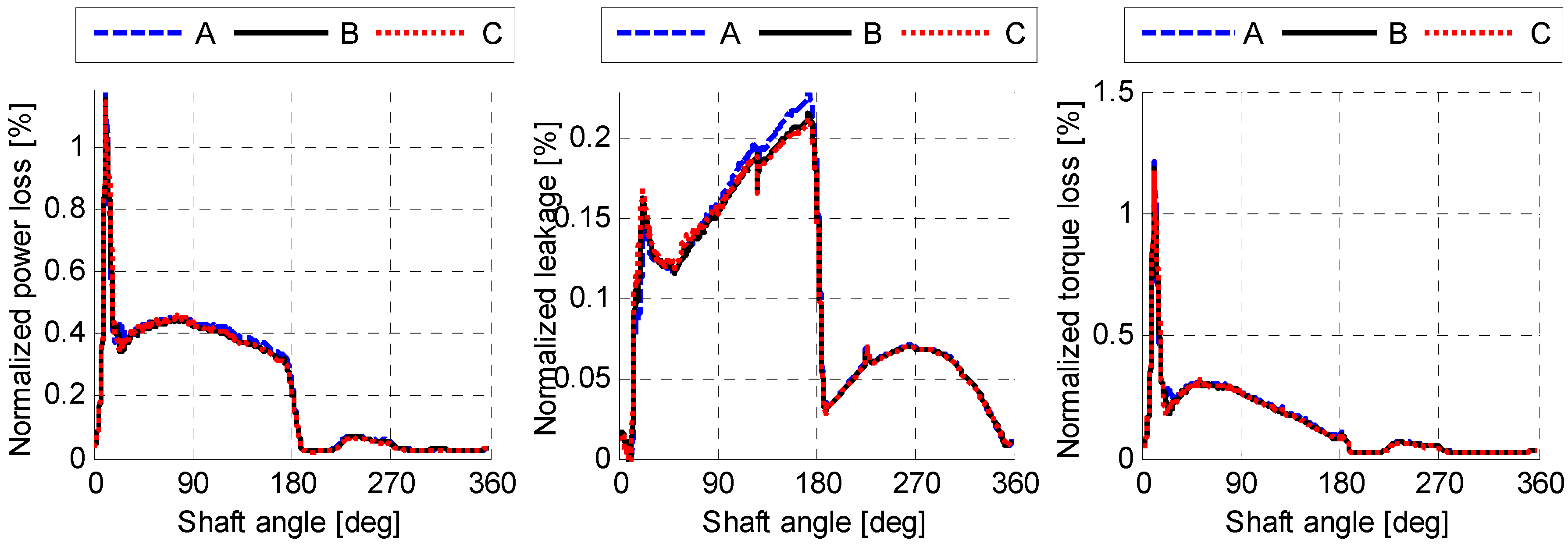
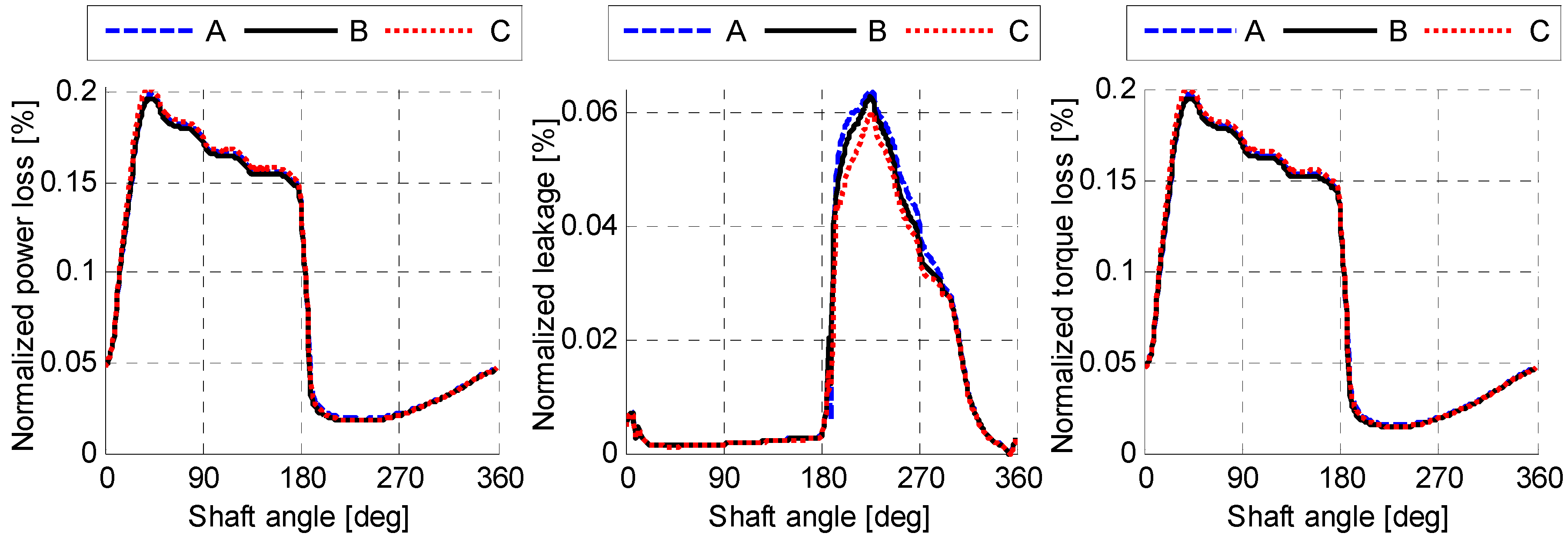
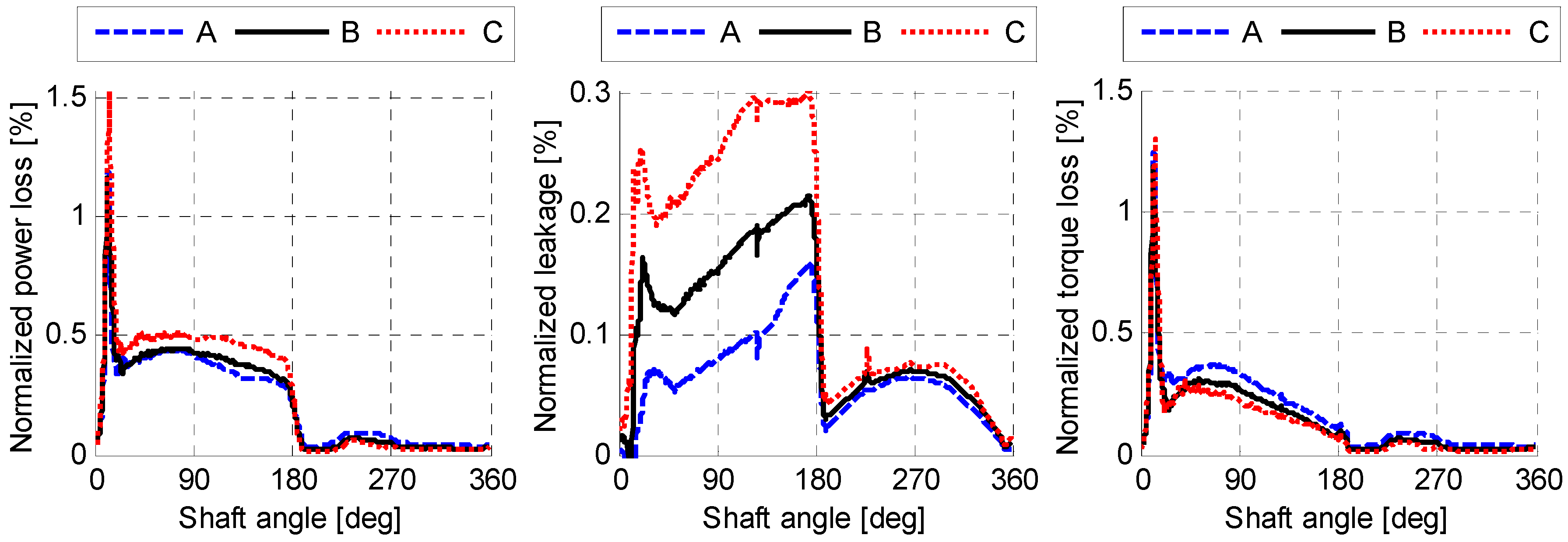
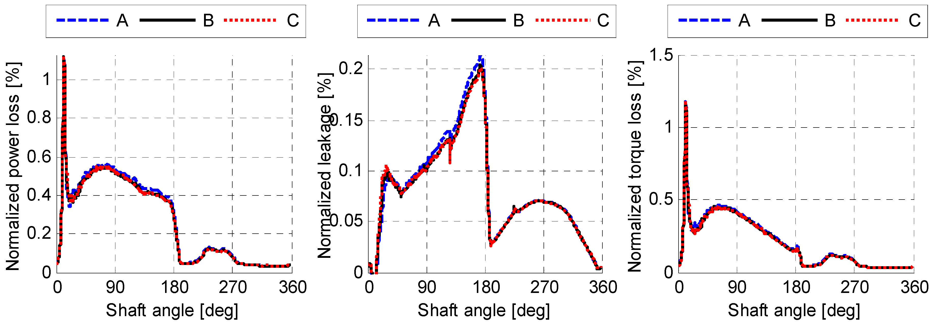
- A size-independent fluid pressure distribution can be achieved by scaling the viscosity with the linear scaling factor. The simulation results in Figure 10, Figure 11 and Figure 12 demonstrated this by showing an identical normalized performance for all three lubricating interfaces when using a scaled viscosity and no heat transfer.
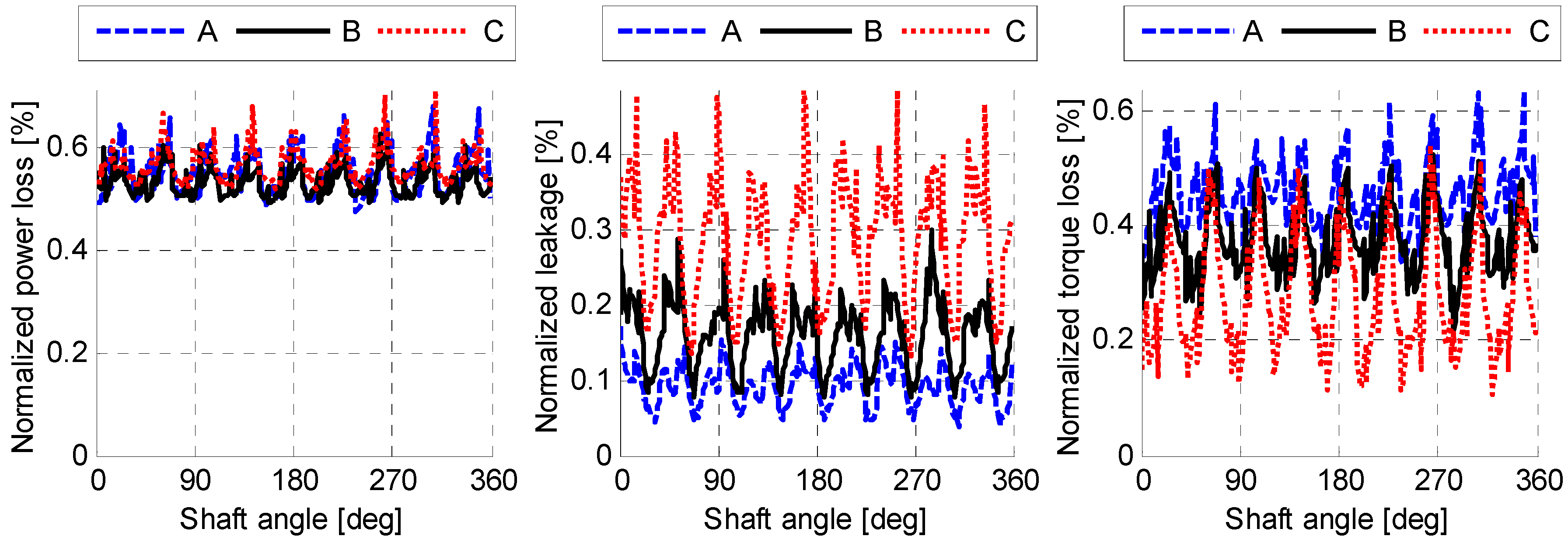
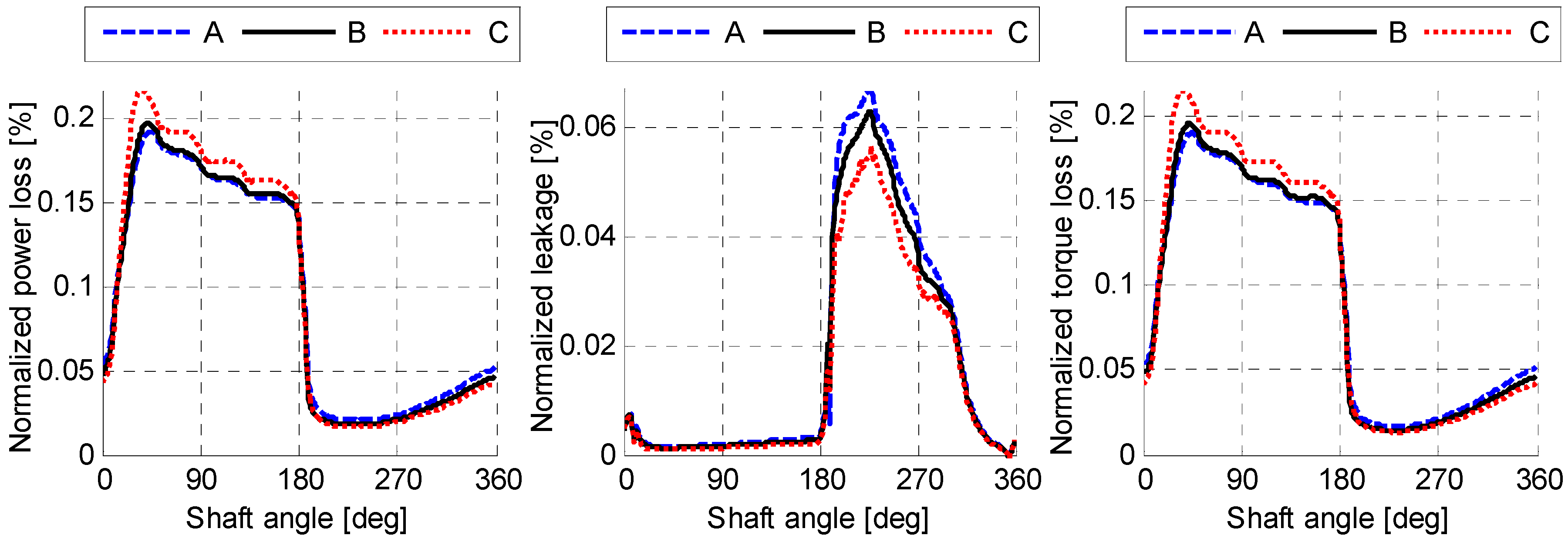
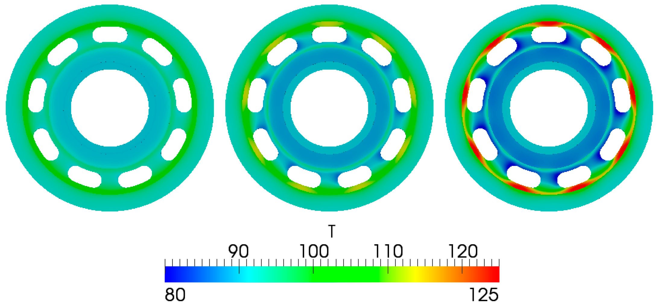
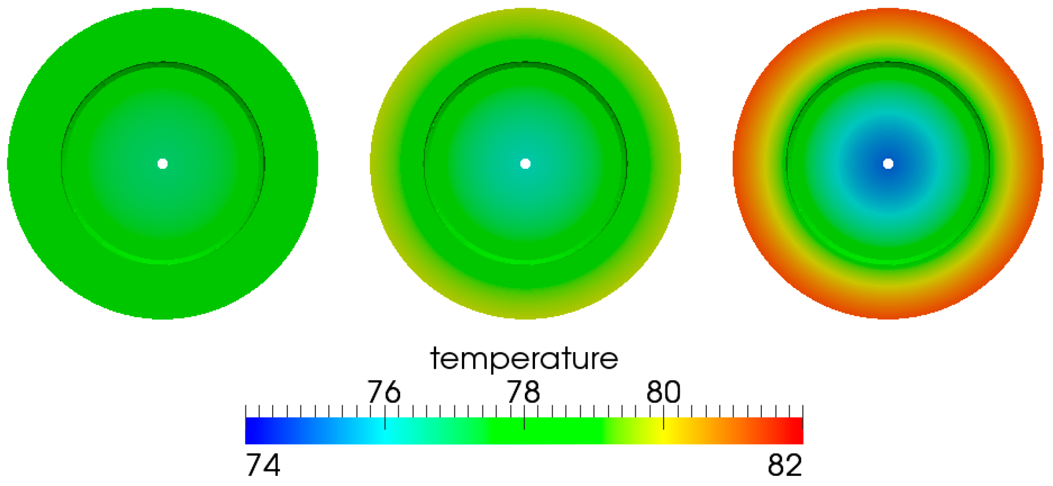
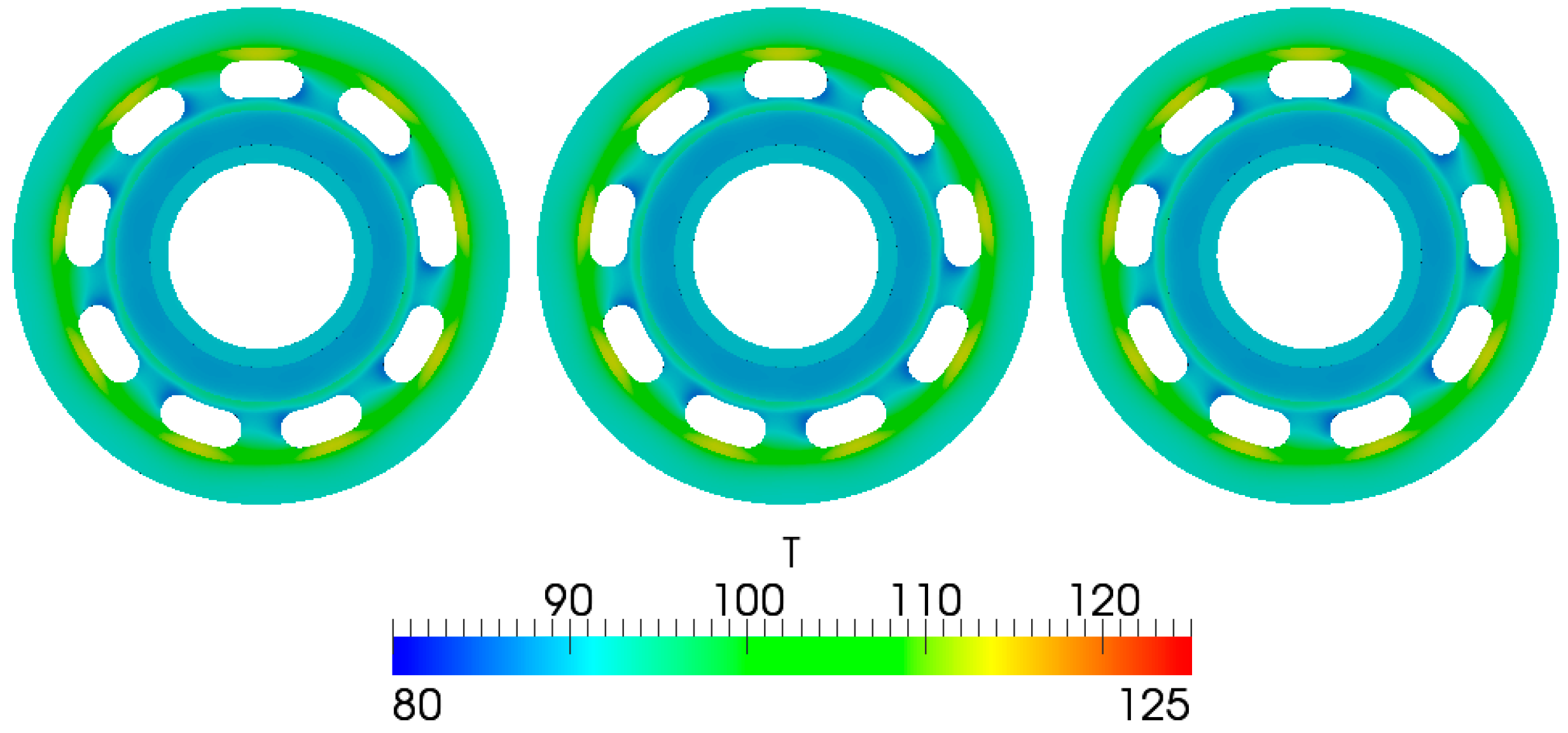
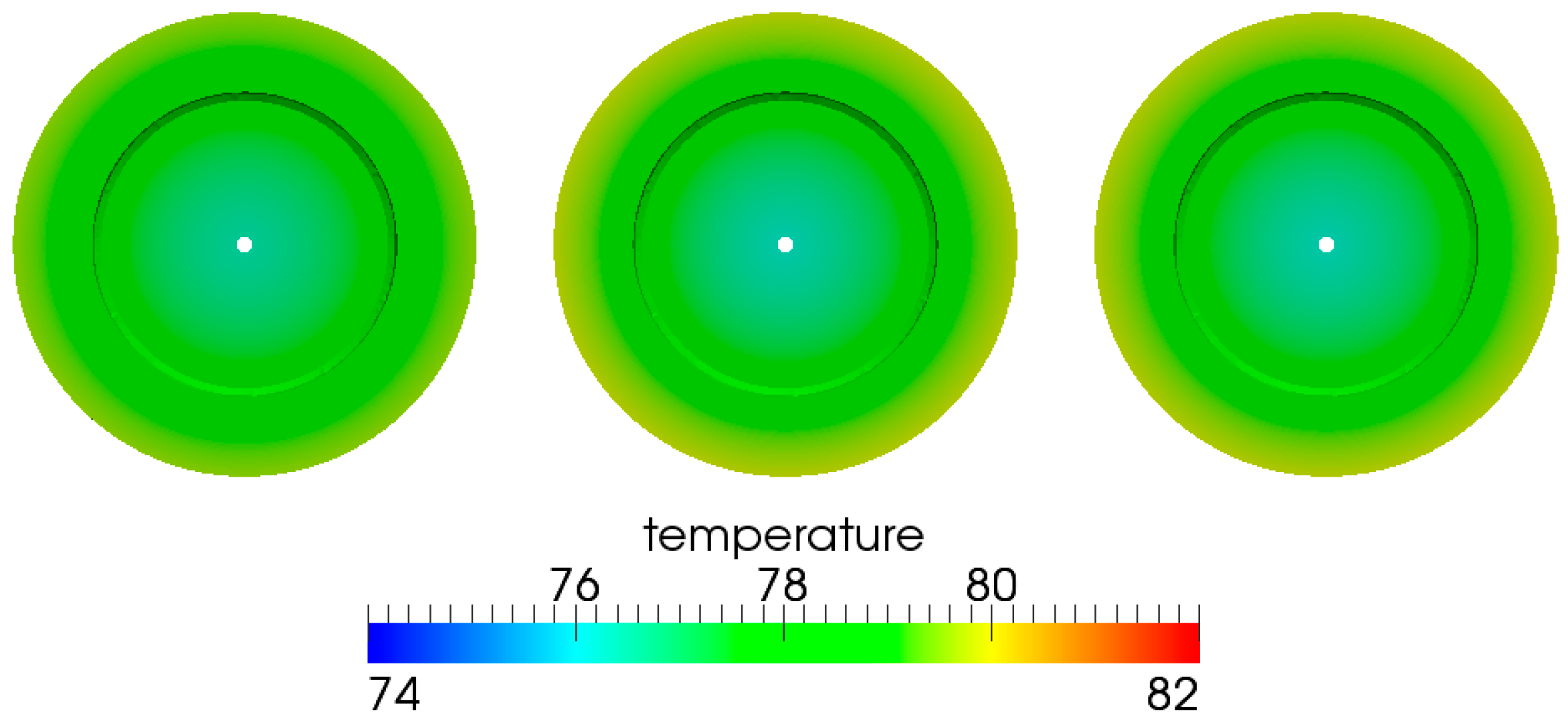
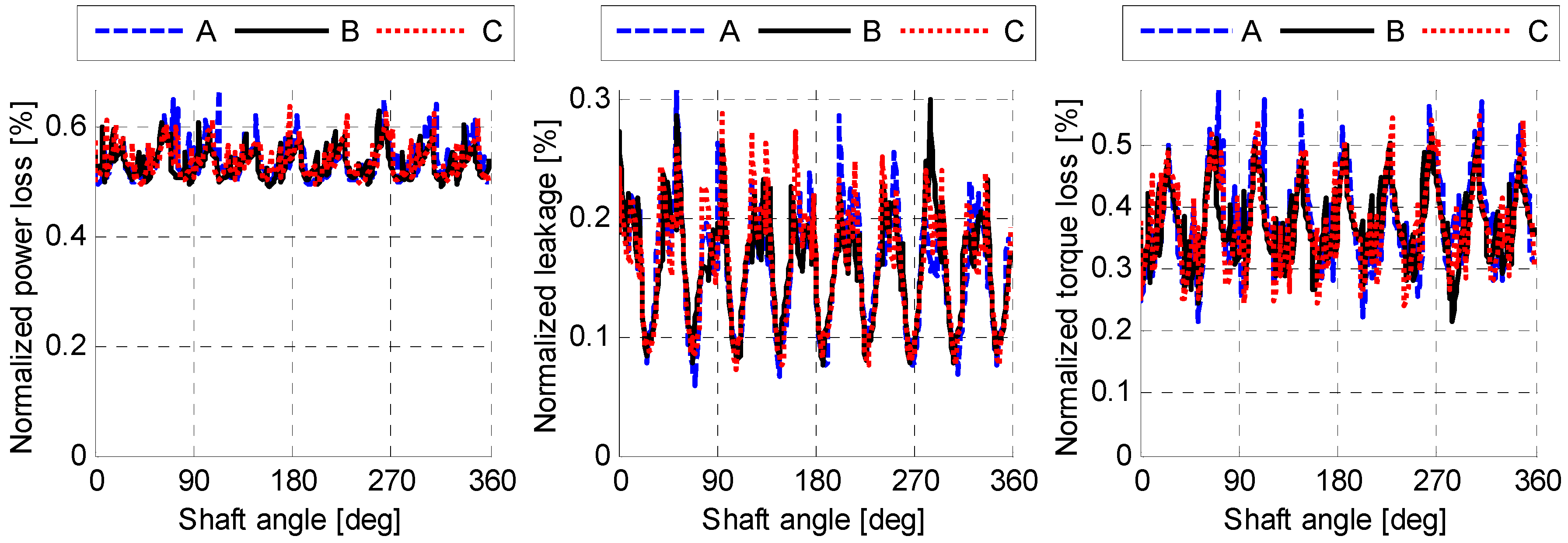
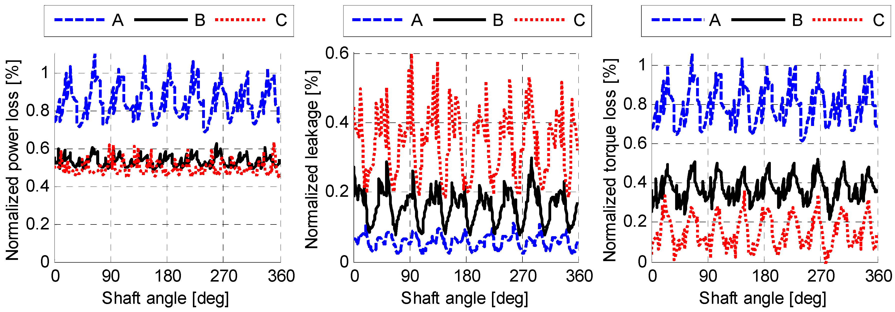
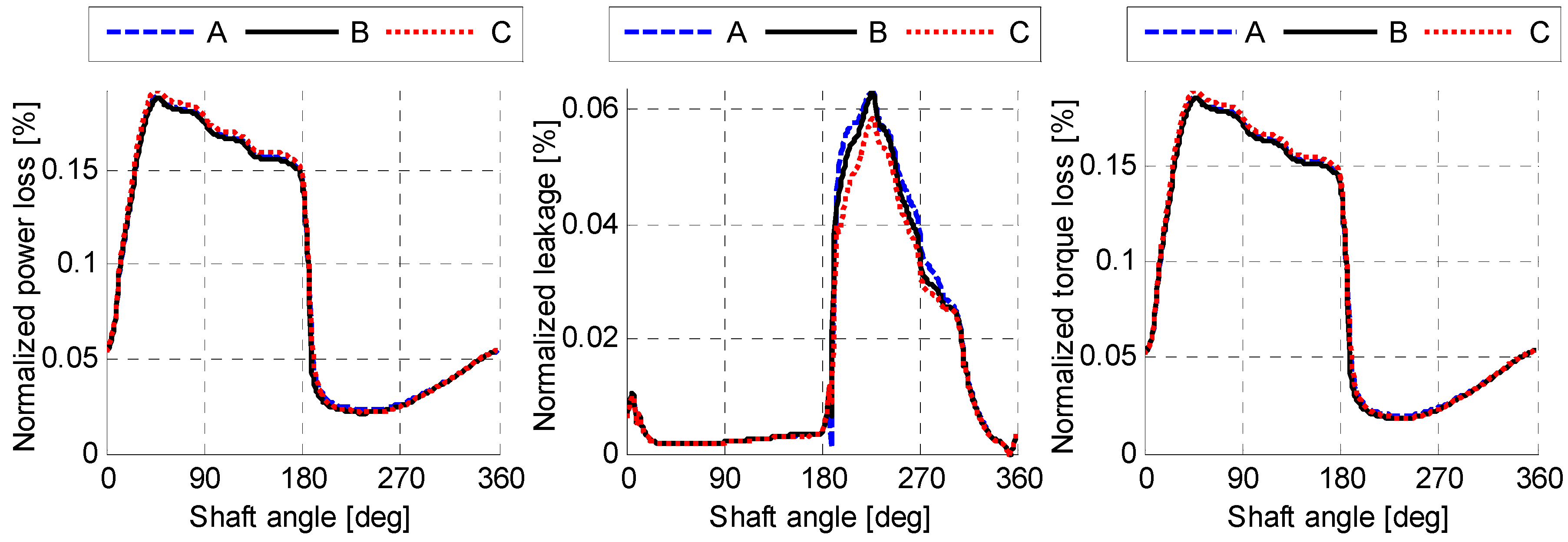
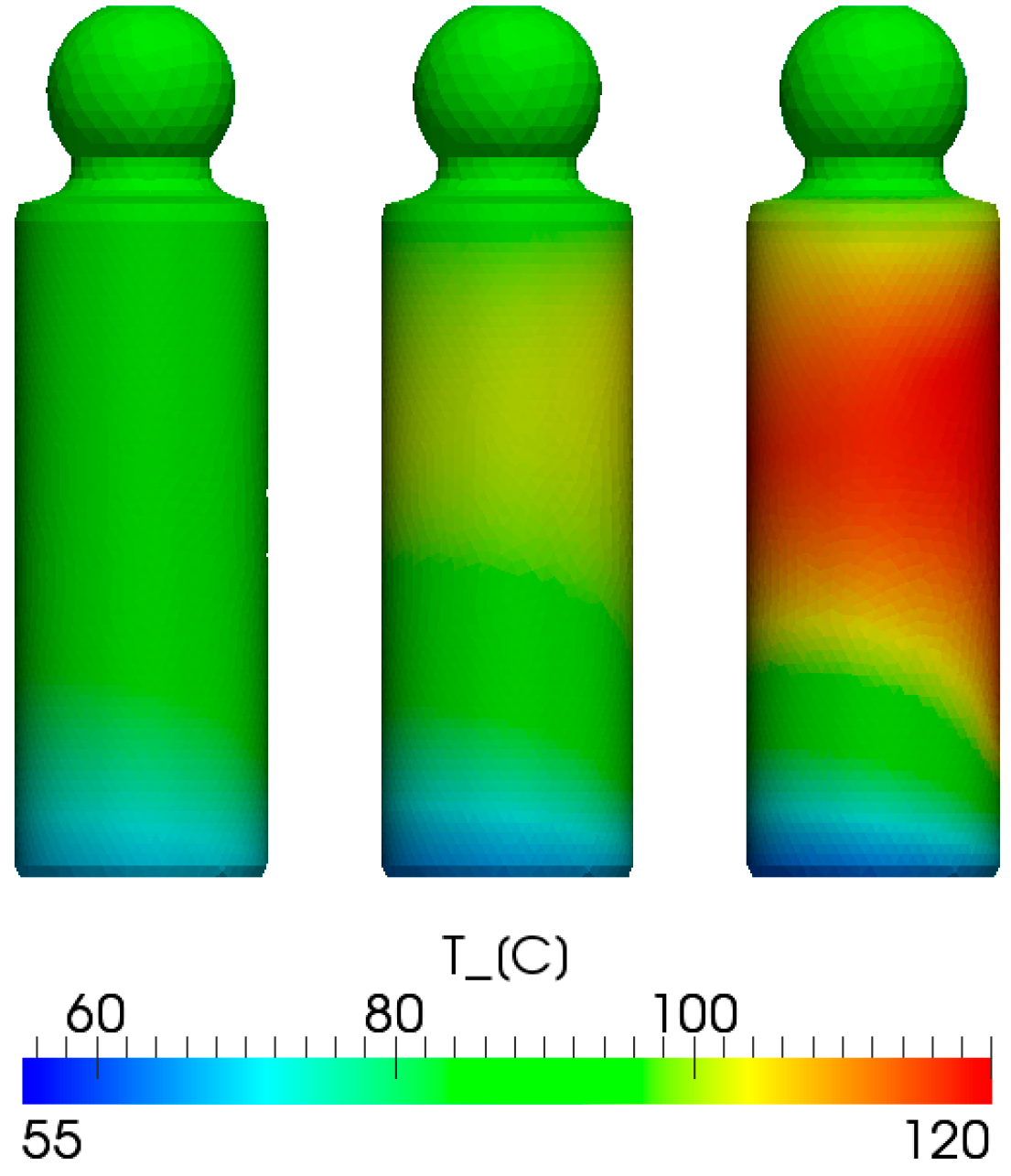
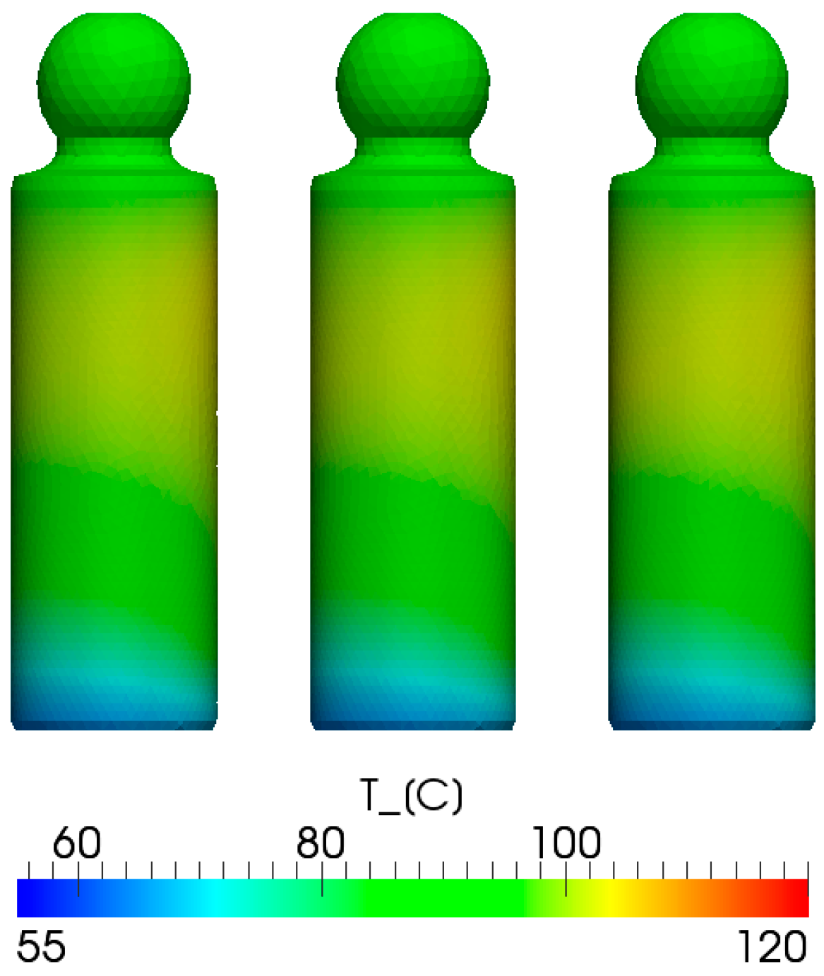
- The size-independent temperature distribution in both the fluid and solid domains can be achieved by scaling the fluid and solid conductivity with the linear scaling factor. The simulation results in Figure 20, Figure 21, Figure 22, Figure 23, Figure 24 and Figure 25 demonstrated this by showing an identical normalized performance for all three lubricating interfaces with a scaled viscosity and conductivity.
- When scaling a swashplate-type axial piston machine to a different size, the size-dependent pressure distribution-induced performance bias can be eliminated by using hydraulic fluid at a different viscosity grade.
- ○
- Use higher viscosity for up-scaling.
- ○
- Use lower viscosity for down-scaling.
- ○
- Choose the viscosity based on the linear scaling factor as in Equation (1).
- The viscosity of the fluid can also be controlled by:
- ○
- Increasing operating temperature for down-scaling
- ○
- Decreasing operating temperature for up-scaling.
- When using a fluid of different viscosity is not feasible, design modifications should compensate for the size-dependent sealing function of the scaled lubricating interfaces:
- ○
- For the piston/cylinder interface, use a lower normalized clearance for up-scaling, and use a higher normalized clearance for down-scaling [28].
- ○
- For the cylinder block/valve plate interface, increase the sealing land area for up-scaling, and decrease the sealing land area for down-scaling [27].
- ○
- For the slipper/swashplate interface, increase the sealing land area for up-scaling, and decrease the sealing land area for down-scaling.
- To compensate for the size-dependent heat transfer, the design of the lubricating interfaces needs to be modified:
- ○
- When up-scaling, the lubricating interface design should be modified in order to increase the cooling performance of the lubricating gap, e.g., adding a flow channel beneath the valve plate to smooth the temperature distribution.
- ○
- When down-scaling, the lubricating interface design should be modified to create more thermal deformation, e.g., by using a bi-material solid body [30].
6. Conclusions
Author Contributions
Funding
Conflicts of Interest
Nomenclature
| Symbols | Denotation | Unit |
| Strain-displacement matrix | ||
| Constitutive matrix | ||
| Diameter | ||
| Vector of nodal force | ||
| Gap height | ||
| Maximum stroke | ||
| Element stiffness matrix | ||
| Length | ||
| Power | ||
| Pressure | ||
| Rate of heat flux | ||
| Stroke | ||
| Temperature | ||
| U | Strain energy | |
| Vector of nodal displacement | ||
| Applied load potential energy | ||
| Speed | ||
| Normal squeezing velocity | ||
| Swashplate angle | ||
| Elastic modulus | ||
| Poisson’s ratio | ||
| Diffusion coefficient | ||
| Vector of elastic strain | ||
| Conductivity | ||
| Linear scaling factor | ||
| Fluid dynamic viscosity | ||
| Total potential energy | ||
| Density | ||
| Vector of elastic stress | ||
| Energy dissipation rate | ||
| Shaft angle | ||
| Shaft speed | ||
| Subscripts | Denotation | |
| Cylinder block | ||
| Bottom surface | ||
| Conductive | ||
| Convective | ||
| Pressure load | ||
| Fluid domain | ||
| Piston | ||
| Optimal | ||
| Solid domain | ||
| Loss due to leakage | ||
| Loss due to friction | ||
| Top surface | ||
| Thermal load | ||
| Pre-scaled |
References
- Ivantysyn, J.; Ivantysynova, M. Hydrostatic Pumps and Motors: Principles, Design, Performance, Modelling, Analysis, Control and Testing; Tech Books International: New Delhi, India, 2003; ISBN 81-88305-08-1. [Google Scholar]
- Merritt, H. Hydraulic Control Systems; John Wiley & Sons: Hoboken, NJ, USA, 1967; ISBN 0-471-59617-5. [Google Scholar]
- Manring, N.D. Friction forces within the cylinder bores of swash-plate type axial-piston pumps and motors. J. Dyn. Syst. Meas. Control 1999, 121, 531–537. [Google Scholar] [CrossRef]
- Manring, N.D. Valve-plate design for an axial piston pump operating at low displacements. J. Mech. Des. 2003, 125, 200–205. [Google Scholar] [CrossRef]
- van der Kolk, H.-J. Beitrag zur Bestimmung der Tragfähigkeit des Stark Verkanteten Gleitlagers Kolben/Zylinder an Axialkolbenpumpen der Schrägscheibenbauart, Verlag Nicht Ermittelbar; Rodenbusch, 1972. [Google Scholar]
- Ivantysynova, M. An Investigation of Viscous Flow in Lubricating Gaps; SVST Bratislava: Bratislava, Slovakia, 1983. [Google Scholar]
- Wieczorek, U.; Ivantysynova, M. Computer aided optimization of bearing and sealing gaps in hydrostatic machines—The simulation tool CASPAR. Int. J. Fluid Power 2002, 3, 7–20. [Google Scholar] [CrossRef]
- Huang, C. An advanced gap flow model considering piston micro motion and elastohydrodynamic effect. In Proceedings of the 4th FPNI PhD symposium, Sarasota, FL, USA, 13–17 June 2006; pp. 181–196. [Google Scholar]
- Pelosi, M.; Ivantysynova, M. The impact of axial piston machines mechanical parts constraint conditions on the thermo-elastohydrodynamic lubrication analysis of the fluid film interfaces. Int. J. Fluid Power 2013, 14, 35–51. [Google Scholar] [CrossRef]
- Pelosi, M.; Ivantysynova, M. A geometric multigrid solver for the piston–cylinder interface of axial piston machines. Tribol. Trans. 2012, 55, 163–174. [Google Scholar] [CrossRef]
- Shang, L.; Ivantysynova, M. Advanced heat transfer model for piston/cylinder interface. In Proceedings of the 11th IFK International Fluid Power Conference, Aachen, Germany, 19–21 March 2018; Volume 1, pp. 587–595. [Google Scholar]
- Shang, L.; Ivantysynova, M. Thermodynamic Analysis on Compressible Viscous Flow and Numerical Modeling Study on Piston/Cylinder Interface in Axial Piston Machine. In Proceedings of the 10th JFPS International Symposium on Fluid Power, Fukuoka, Japan, 24–27 October 2017; pp. 475–581. [Google Scholar]
- Sartchenko, J.S. Force Balance Condition of the Valve Plate and Rotor of an Axial Piston Pump; British Hydromechanics Research Association: Bingley, UK, 1950; p. 10. [Google Scholar]
- Franco, N. Pump design by force balance. Hydraul. Pneum. 1961, 14, 101–107. [Google Scholar]
- Zecchi, M.; Ivantysynova, M. A novel fluid structure interaction model for the cylinder block/valve plate interface of axial piston machines. In Proceedings of the 52nd National Conference on Fluid Power, Las Vegas, NV, USA, 23–25 March 2011. [Google Scholar]
- Zecchi, M.; Ivantysynova, M. A novel approach to predict the cylinder block/valve plate interface performance in swash plate type axial piston machines. In Proceedings of the ASME/Bath Symposium on Fluid Power and Motion Control, Valencia, Spain, 8–12 July 2012; pp. 13–28. [Google Scholar]
- Zecchi, M. A Novel Fluid Structure Interaction and Thermal Model to Predict the Cylinder Block/Valve Plate Interface Performance in Swash Plate Type Axial Piston Machines; Purdue University: West Lafayette, IN, USA, 2013. [Google Scholar]
- Shute, N.A.; Turnbull, D.E. The Minimum Power Loss of Hydrostatic Slipper Berrings; BHRA: Bingley, UK, 1962. [Google Scholar]
- Shute, N.A.; Turnbull, D.E. The Losses of Hydrostatic Slipper Bearings under Various Operating Conditions; British Hydromechanics Research Association: Bingley, UK, 1962. [Google Scholar]
- Hooke, C.J.; Li, K.Y. The lubrication of overclamped slippers in axial piston pumps—Centrally loaded behaviour. Proc. Inst. Mech. Eng. Part C 1988, 202, 287–293. [Google Scholar] [CrossRef]
- Hooke, C.J.; Li, K.Y. The lubrication of slippers in axial piston pumps and motors—The effect of tilting couples. Proc. Inst. Mech. Eng. Part C 1989, 203, 343–350. [Google Scholar] [CrossRef]
- Schenk, A.; Ivantysynova, M. The influence of swashplate elastohydrodynamic deformation. In Proceedings of the 7th FPNI PhD Symposium, Reggio Emilia, Italy, 27–30 June 2012. [Google Scholar]
- Schenk, A.; Ivantysynova, M. A transient thermoelastohydrodynamic lubrication model for the slipper/swashplate in axial piston machines. J. Tribol. 2015, 137, 031701. [Google Scholar] [CrossRef]
- Schenk, A.; Ivantysynova, M. An investigation of the impact of elastohydrodynamic deformation on power loss in the slipper swashplate interface. In Proceedings of the 8th JFPS International Symposium on Fluid Power, Okinawa, Japan, 25–28 October 2011. [Google Scholar]
- Schenk, A.T. Predicting Lubrication Performance between the Slipper and Swashplate in Axial Piston Hydraulic Machines; Purdue University: West Lafayette, IN, USA, 2014. [Google Scholar]
- Shang, L.; Ivantysynova, M. Port and case flow temperature prediction for axial piston machines. Int. J. Fluid Power 2015, 16, 35–51. [Google Scholar]
- Shang, L.; Ivantysynova, M. An Investigation of Design Parameters Influencing the Fluid Film Behavior in Scaled Cylinder Block/Valve Plate Interface. In Proceedings of the 9th FPNI PhD Symposium on Fluid Power; American Society of Mechanical Engineers, Florianópolis, SC, Brazil, 26–28 October 2016; p. V001T01A027. [Google Scholar]
- Shang, L.; Ivantysynova, M. A Path toward Effective Piston/Cylinder Interface Scaling Approach. In Proceedings of the ASME/BATH 2017 Symposium on Fluid Power and Motion Control, Sarasota, FL, USA, 16–19 October 2017; p. V001T01A072. [Google Scholar]
- Reynolds, O. IV. On the theory of lubrication and its application to Mr. Beauchamp tower’s experiments, including an experimental determination of the viscosity of olive oil. Philos. Trans. R. Soc. Lond. 1886, 177, 157–234. [Google Scholar] [CrossRef] [Green Version]
- Shang, L.; Ivantysynova, M. A temperature adaptive piston design for swash plate type axial piston machines. Int. J. Fluid Power 2017, 18, 38–48. [Google Scholar] [CrossRef]


| A | B | C | |
|---|---|---|---|
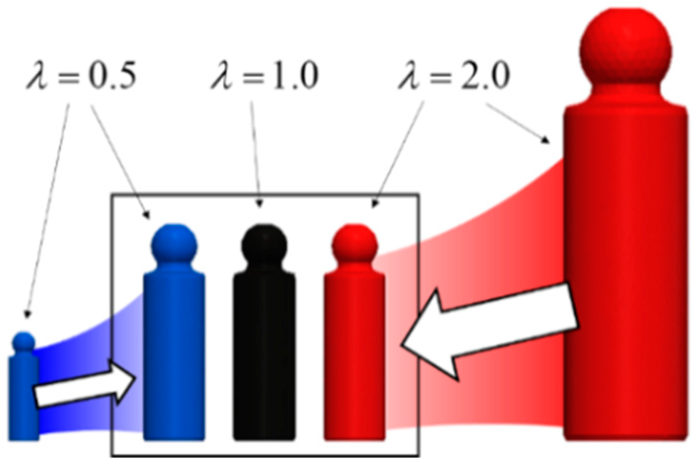
| Linear factor | 0.5 | 1 | 2 |
| Unit size [cc] | 9.375 | 75 | 600 |
| Pressure [bar] | 400 | 400 | 400 |
| Displacement [%] | 100 | 100 | 100 |
| Speed [rpm] | 7200 | 3600 | 1800 |
| A | B | C | |
|---|---|---|---|
| Linear factor | 0.5 | 1 | 2 |
| Unit size [cc] | 9.375 | 75 | 600 |
| Pressure [bar] | 400 | 400 | 400 |
| Displacement [%] | 100 | 100 | 100 |
| Speed [rpm] | 7200 | 3600 | 1800 |
| Fluid viscosity |
| A | B | C | |
|---|---|---|---|
| Linear factor | 0.5 | 1 | 2 |
| Unit size [cc] | 9.375 | 75 | 600 |
| Pressure [bar] | 400 | 400 | 400 |
| Displacement [%] | 100 | 100 | 100 |
| Speed [rpm] | 7200 | 3600 | 1800 |
| Fluid viscosity | |||
| Fluid conductivity | |||
| Solid conductivity |
© 2018 by the authors. Licensee MDPI, Basel, Switzerland. This article is an open access article distributed under the terms and conditions of the Creative Commons Attribution (CC BY) license (http://creativecommons.org/licenses/by/4.0/).
Share and Cite
Shang, L.; Ivantysynova, M. Scaling Criteria for Axial Piston Machines Based on Thermo-Elastohydrodynamic Effects in the Tribological Interfaces. Energies 2018, 11, 3210. https://doi.org/10.3390/en11113210
Shang L, Ivantysynova M. Scaling Criteria for Axial Piston Machines Based on Thermo-Elastohydrodynamic Effects in the Tribological Interfaces. Energies. 2018; 11(11):3210. https://doi.org/10.3390/en11113210
Chicago/Turabian StyleShang, Lizhi, and Monika Ivantysynova. 2018. "Scaling Criteria for Axial Piston Machines Based on Thermo-Elastohydrodynamic Effects in the Tribological Interfaces" Energies 11, no. 11: 3210. https://doi.org/10.3390/en11113210
APA StyleShang, L., & Ivantysynova, M. (2018). Scaling Criteria for Axial Piston Machines Based on Thermo-Elastohydrodynamic Effects in the Tribological Interfaces. Energies, 11(11), 3210. https://doi.org/10.3390/en11113210