Computer Simulation of Temperature Distribution during Cooling of the Thermally Insulated Room

Abstract

This paper is devoted to modelling of temperature distribution and its time evolution in rooms with specific thermal insulation and heat transfer for different external conditions. The simulation results should help to design the room architecture and wall materials to reduce energy losses due to heating or cooling, and to increase the inside thermal comfort. For this purpose, a methodological procedure using real data processing in the COMSOL Multiphysics modelling environment and spatial visualization of temperature evolution is proposed. This paper describes a mathematical model for simulation of the temperature evolution inside a space with thermally insulated walls under selected outside conditions. Computer simulations are then used to assess the temperature distribution inside the room and the heat flow through the room walls. Results of the simulations are used for subsequent determination of the time needed for the desired decrease of air temperature inside the tested room during its cooling due to the low ambient temperature, which is related to the thermal stability of the building, specific heat capacity, and thickness of the thermal insulation. Under the studied conditions, the time to reach the temperature drops by 20 percent in a room with windows was from 1.4 to 1.8 times lower than that in the room without windows. The proposed methodology shows the flexibility of computer modelling in the design of insulated building systems. The mesh density testing was performed by comparing the air temperature evolution in the model of the selected mesh density and the model with its maximum value enabled by the size of computer memory. The maximum temperature deviation calculated for the mesh of the presented model was 0.57%.

1. Introduction

Urban areas are developing rapidly from a technological viewpoint [1]. Nowadays, over half of the world’s population live in cities. Furthermore, the ongoing trend toward urbanisation will create a staggering increase in city populations of 2.8 billion by 2050. The constant increase in population living in cities has led to increased energy demands from households. Apart from industry and transport, households are currently major energy consumers. Heating accounts for the biggest energy and fuel consumption in European households. Its consumption ranged between 60 and 70% in most European Union counties in 2014, which is a leading cause of global warming.

Reducing the carbon dioxide emissions produced by households is another reason for creating the concept of smart cities, which use smart, meaningful and gentle modern technology and approaches to improve life, to manage energy more effectively, to conserve natural resources and ensure energy sustainability [2]. An integral part of smart cities will be smart buildings, which will utilise monitoring devices that will track usage, and empower users and service providers to better control and reduce energy demand [3,4,5].

Minimising the energy demands of buildings needs to be focused on when designing new buildings and during house renovations [6,7]. The thermal stability of buildings depends on both the thermal stability of the building’s shell and the heat capacity of the internal structures and equipment. The heat resistance of buildings can also be significantly influenced by the appropriate thermal insulation of their walls by a suitable heat-insulating material that can reduce heat losses in winter and undesirable heating in summer [8,9]. Phase change materials can also be used as passive energy storage for building systems [10]. The impact of coupled heat and moisture transfer affects a building’s energy consumption [11]. Testing the optimal thermal performance of buildings requires us to model the energy transfer between a building and its surroundings. However, solving the problems of heat transfer in buildings is very challenging. Various heat exchange processes are possible between the indoor building environment and the external environment. The heat flow is conducted by the walls, roof, ceiling, floor, and so on. Heat transfer also takes place on different surfaces by convection and radiation. Heat is also added to space due to the presence of human occupants, and due to the use of lights and equipment [12].

Many building energy simulation programs (e.g., BLAST, DeST, DOE-2, ECOTECT, IES, EnergyPlus, TAS, TRNSYS, FLUENT, ESP-r [13], etc.) have been developed over the past few decades [14,15,16,17]. However, the code for energy simulation in buildings often uses heat transfer models based on a one-dimensional heat flow, which can give unreliable results or can calculate only stationary processes [18]. Therefore, the TRNSYS software (18, University of Wisconsin-Madison, Madison, WI, USA) is designed mainly to assess the performance of thermal and electrical energy systems under transient conditions. In addition, SolidWorks Flow Simulation software was tested as a possible tool for modelling the energy balance in building structures [19]. Compared with this software, the current version of COMSOL Multiphysics (5.3, COMSOL, Inc., Stockholm, Sweden) includes modules which allow simultaneous assessment of the heat and mass transfer for both stationary and time-dependent processes. In this regard, the paper by [20] deals with a two-dimensional transient modelling of energy and mass transfer in the porous building components using COMSOL Multiphysics. The authors in [21] deal with the study of moisture hysteresis influence on mass transfer through bio-based building materials in dynamic state. In [22], COMSOL Multiphysics was used for testing of an impact of paper and wooden collections on humidity stability and energy consumption in museums and libraries humidity stability and energy consumption. Similarly, in [23], the multiphysics modelling of heat and moisture induced stress and strain of historic building materials and artifacts was tested. The paper by [24] presents a renewed approach to the development of two layers super-insulated precast concrete structural sandwich panels using the thermal path method. The heat transfer was experimentally measured and the results were verified using a 3D component of COMSOL Multiphysics software. The research by [25] aims at simulating the process of spatial heat transfer in a multilayer non-uniform structure of an external cast-in-place framed wall produced from polystyrene concrete with a stay-in-place formwork. Based on the physico-mathematical model developed with the use of ANSYS and COMSOL software complexes, parametric analysis of the impact of various factors on thermal behavior of the external wall was performed with the account of heat-stressed frame elements. Meanwhile, the authors in [26] present results of the investigation of evaporation cooling on drying capillary active building materials by numerical simulation and non-destructive measurements. The paper by [27] presents an investigation regarding the effect of indoor thermal to building’s occupant satisfaction in a building that is mechanically ventilated. The study by [28] deals with the transient heat transfer in a multi-layered building wall through the facades of the buildings located in the city of Bechar in southwest Algeria. This physical model was presented to find the variation of the transient temperature in these structures and the heat flux through these elements, which depends on the air temperature of the inner surface and the instantaneous climatic conditions of the air outside. A combined finite element analysis and experimental validation approach to estimating effective edge conductivities of vacuum insulation panels embedded in foam-VIP composites is presented in [29]. An integral component of numerical simulation using finite elements is the boundary conditions, which, in the case of simulating the thermal performance of a building element, are usually expressed in terms of the external surface temperature as a function of time. The purpose of this study is to examine the effect of the accuracy of the boundary conditions on the thermal performance simulation of building elements.

In study [30], the possibility of using COMSOL Multiphysics in simulations of the heat transfer in a building environment was verified by comparative Building Energy Simulation Test (“BESTEST”) [31], which is a methodology that was developed by the International Energy Agency and that was used for systematically testing whole building energy simulation programs and diagnosing sources of predictive disagreement. An accuracy of the room model presented in this paper was verified by experimental testing on a real room with the same construction as the construction of a model formulated in the COMSOL Multiphysics interface. Comparison of the data obtained by computer simulation for this model with data obtained by experimental testing is presented in [32].

In addition to the computational kernel that enables complex multiphysical tasks, the current COMSOL Multiphysics version offers the Application Builder interface, which enables us to quickly create easy-to-use applications based on working models [33]. From this aspect, we intend to use COMSOL Multiphysics to create a complex software tool for the assessment of energy performance of selected models of building parts. Simultaneously, we would like to ensure the possibility of universal use of this tool, not only for specialists who are trained to control the software but also for external users via a web interface [32]. For this purpose, we are preparing a set of room modules in which users can specify both geometric and physical properties.

In this paper, we follow the paper [34], which presents the interim results of the research on the developing methodological procedure which could be used for assessment of the thermal stability of buildings with regards to their thermal accumulative parameters concerning compliance with valid European technical standards [35] used in building industry and architecture. We describe computer application programmed in the Application Builder of the COMSOL Multiphysics software, which can simulate cooling of a room as a 3D model under the selected winter condition. The first part of this paper includes the theoretical background of the studied problem. The second part describes a model of the studied room. The following parts demonstrate the use of the proposed computer application by testing the thermal stability of the room in case of its cooling concerning the outside wall’s thermal insulation properties.

The aim of the simulations is to assess the temperature distribution of air inside the room and the heat losses in the winter season dependent on thermophysical properties of a thermal insulation of the outside wall. The Heat Transfer Module of COMSOL Multiphysics 5.3 [36] with the laminar flow was used to build a model of the tested room. This provides several tools for modelling coupled heat transport in building materials and adjacent air domains by taking into account heat storage and latent heat effects. Its computing core is based on numerical solving of the studied models by using the finite element method.

2. Model Description

The basic parameterised 3D model of the studied room was first formulated and tested by the standard Model Builder of COMSOL Multiphysics. Its geometric layout is shown in Figure 1. This pilot model includes only the basic elements that influence heat transfer between inside and outside environments. Therefore, it consists of side walls, floor, windows, doors and thermally insulated ceiling and outside wall with thermal insulation under the window. It also includes two heaters, which are needed to test the heat transfer in the case of heating the room. The model supposes that the tested room is surrounded by two neighboring rooms and by another one below. There is a corridor behind the wall with the door. The dimensions of all elements can be changed as required.

Because of assumed time-dependent temperature distributions of all of the elements of the model, and also variable temperatures of air inside and outside the room, the studied problem has to be solved as non-stationary heat transfer using relation [37] to describe these processes:

$$\nabla \left(-\lambda \nabla T\right)+\varrho c_{p}v\nabla T+\varrho c_p\frac{\partial T}{\partial t}=\mathsf{\Phi },$$

(1)

where symbol $\varrho$ stands for the material density, $c_p$ is the specific heat capacity, T denotes the temperature, t is the time, v is the fluid velocity, $\lambda$ is the thermal conductivity, and $\mathsf{\Phi }$ denotes the inner heat-generation rate per unit volume.

The first part of the Equation (1) describes heat transfer by conduction in solids. The second part describes heat convection in fluids, and the third part describes heat accumulation in the mass of a specific domain. The sum of these processes is equal to the domain heat source.

It is assumed that the boundary conditions can be of the following types [37,38]:

• Specified temperature ($T_s$) on a surface: $T_s=T\left(x,y,z,t\right).$
• Heat flow density $\left(q_s\right)$ on a surface: $q_s=q(x,y,z,t).$
• Convective boundary condition: $q_x{n}_x+q_y{n}_y+q_z{n}_z=h\left(T_s-T_e\right)+q_r.$

Symbol h stands for the heat transfer coefficient, $T_s$ denotes the surface temperature, $T_e$ is the convective exchange temperature, $q_r$ denotes the incident radiant heat flow per unit surface area, and $q_x$, $q_y$, $q_z$ are components of the heat flow density.

Finally, for the initial temperature field of a body at the time $t=0$, it holds [37]

$$T\left(x,y,z,t\right)=T_0\left(x,y,z\right),$$

(2)

where $T_0$ stands for the initial temperature of the body.

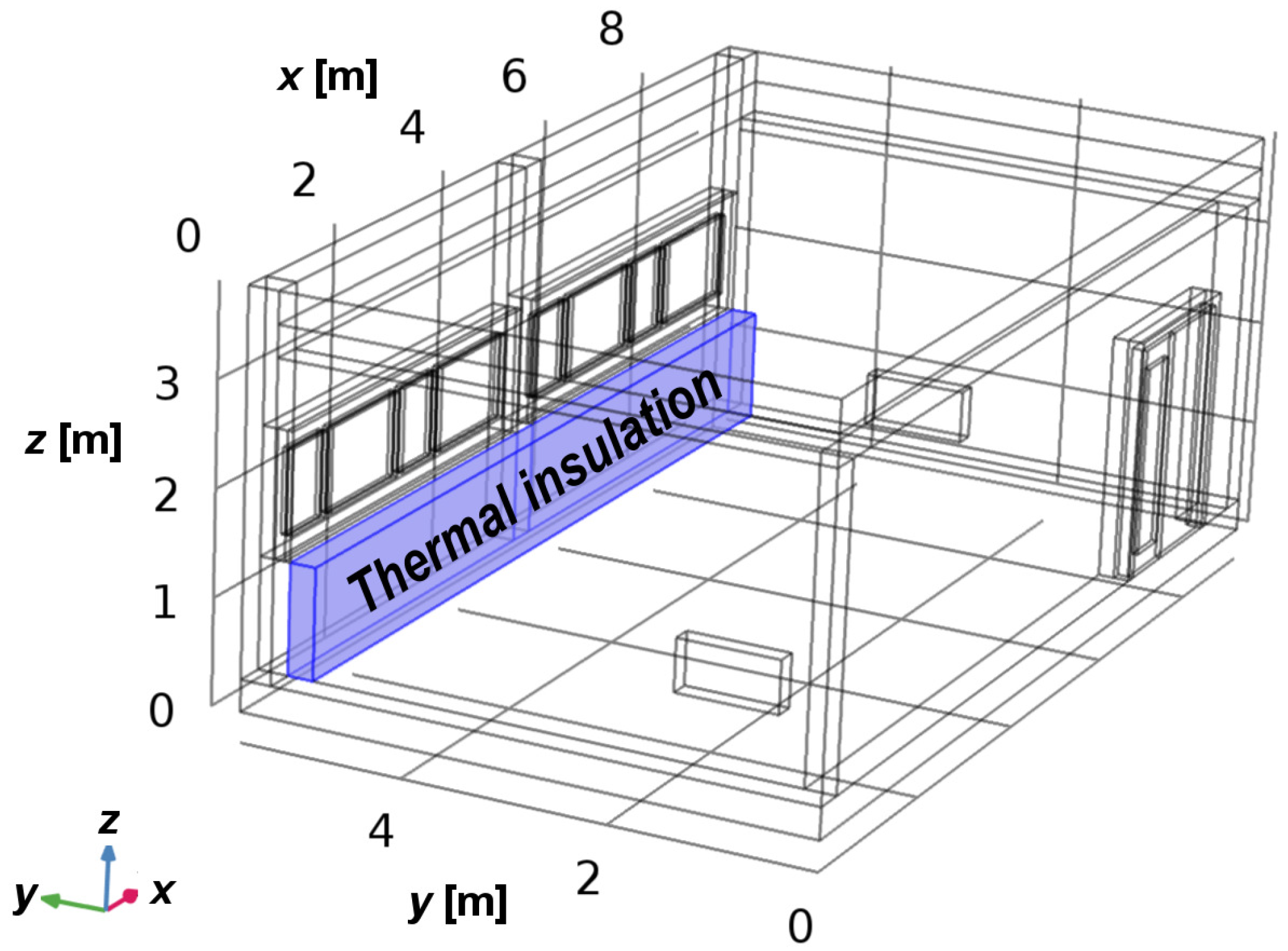
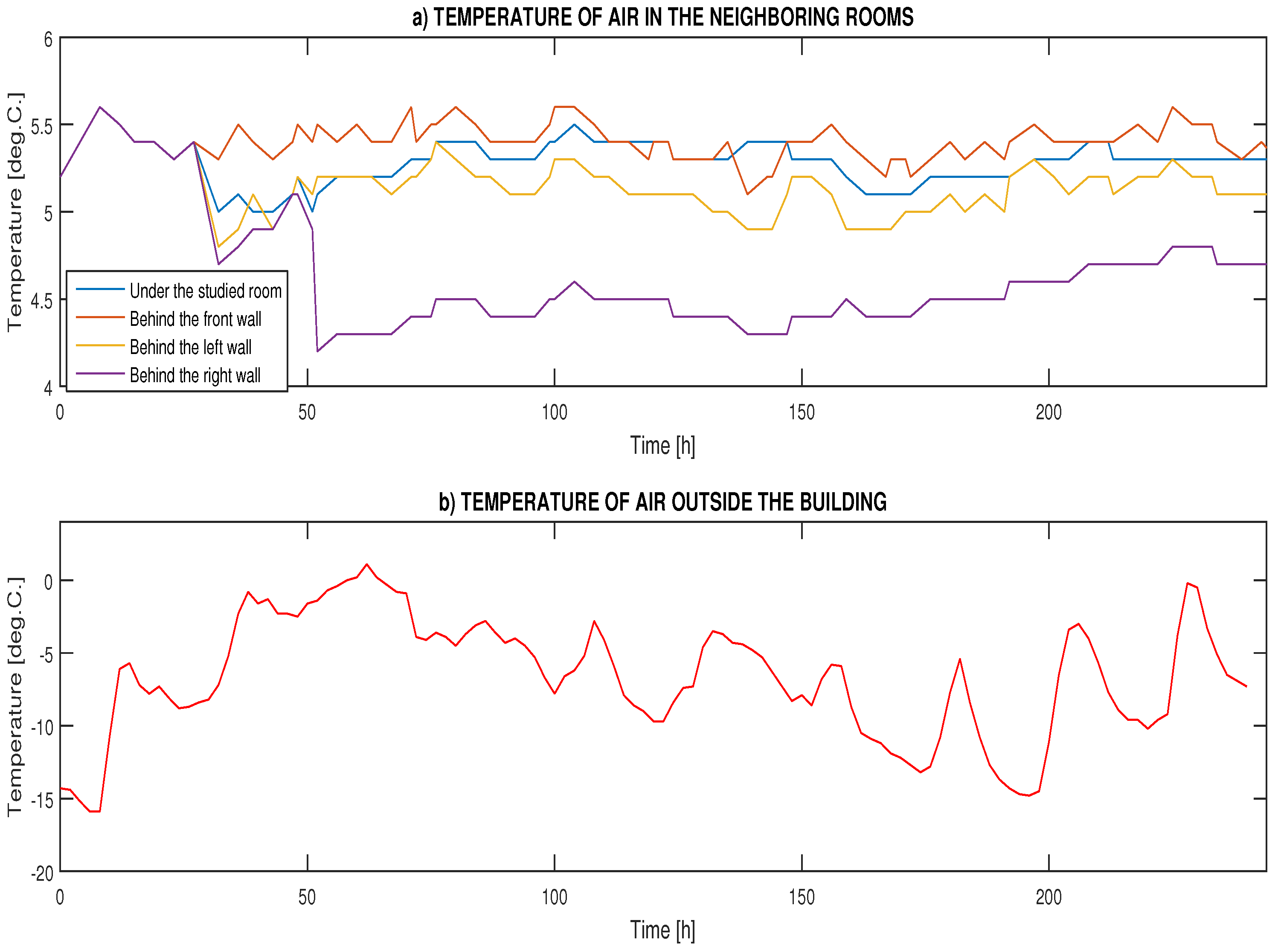
2.1. Simulation Conditions

Size and physical properties of the geometrical elements of the tested room are listed in

Table 1. Size and physical properties of geometrical elements of the studied room.

Geometrical Element	Size $\left[\mathbf{m}\right]$	Thermal Conductivity $\left[\mathbf{W}·{\mathbf{m}}^{-1}·{\mathbf{K}}^{-1}\right]$	Density $\left[\mathbf{kg}·{\mathbf{m}}^{-3}\right]$	Specific Heat Capacity $\left[\mathbf{J}·{\mathbf{kg}}^{-1}·{\mathbf{K}}^{-1}\right]$	Emissivity $\left[1\right]$
Rear wall	$8.7\times 0.3\times 3$	0.27	900	960	0.85
Left side wall	$5\times 0.3\times 3$	0.27	900	960	0.85
Right side wall	$5\times 0.3\times 3$	0.27	900	960	o.85
Wall under the windows	$8.4\times 0.3\times 1.05$	0.80	1700	900	0.80
Wall above the windows	$8.4\times 0.3\times 0.75$	0.80	1700	900	0.80
Columns in the outside wall	$0.3\times 0.3\times 3$	0.32	2192	1018	0.85
Floor	$8.7\times 5\times 0.3$	1.43	2300	1020	0.85
Ceiling	$8.7\times 5\times 0.3$	0.82	1251	1021	0.8
Insulation above the ceiling	$8.7\times 5\times 0.3$	0.04	30	1270	0.90
Insulation of the outside wall	$8.7\times variable\times 1.05$	0.05	3000	1500	0.85
Window frames	$4.2\times 0.145\times 1.2$	0.18	400	2510	0.89
Glass in larger windows	$1.2\times 0.008\times 0.8$	0.76	2600	840	0.99
Glass in smaller windows	$0.6\times 0.008\times 0.8$	0.76	2600	840	0.99
Door leaf	$1\times 0.05\times 2.2$	0.11	800	1150	0.89
Panel next to the door	$0.65\times 0.05\times 2.2$	0.20	1380	1100	0.94
Door frame	$1.85\times 0.1\times 2.3$	58	7850	440	0.89
Door trim	$0.45\times 0.05\times 1.8$	0.76	2600	840	0.9
Left heater	$0.2\times 0.5\times 1$	58	7850	440	0.88
Right heater	$0.2\times 0.5\times 1$	58	7850	440	0.88

. Figure 2 presents the temperature of air in the adjoining rooms and the temperature of the air outside the building.

Further conditions, geometry and material properties of the studied model include:

• Room dimensions: length 8.7 m, width 5 m, height 3 m.
• The initial temperature of the air inside the tested room $21{}^{°}\mathrm{C}$.
• Temperature of air in the adjoining rooms of the building $0{}^{°}\mathrm{C}$.
• Velocity of the airflow inside the tested room $0.03\mathrm{m}·{\mathrm{s}}^{-1}$.
• Heat transfer coefficient inside the building $8\mathrm{W}·{\mathrm{m}}^{-2}·{\mathrm{K}}^{-1}$.
• Heat transfer coefficient outside the building $25\mathrm{W}·{\mathrm{m}}^{-2}·{\mathrm{K}}^{-1}$.

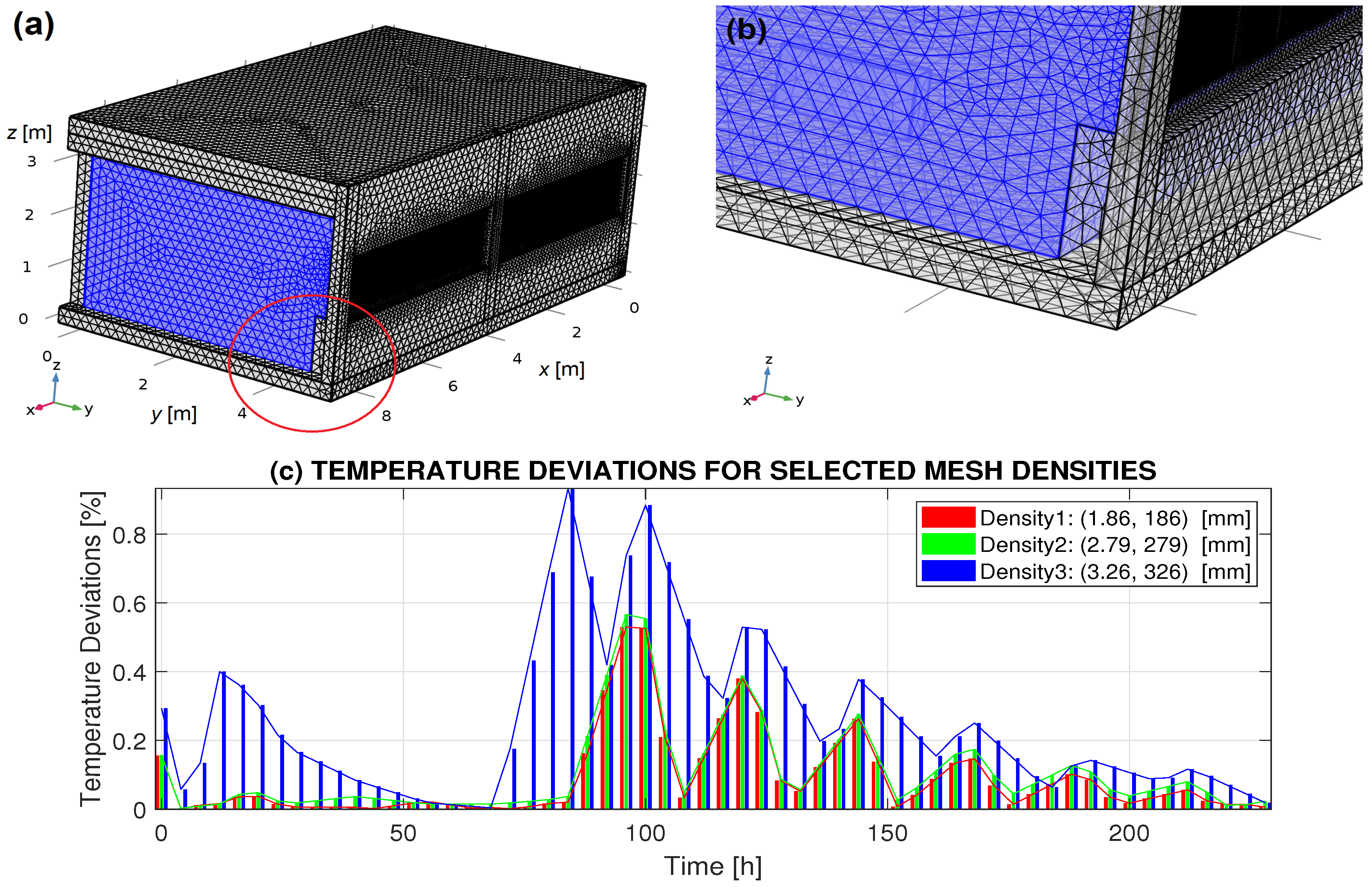
2.1.1. Domain Setting

In the presented room model, the heat energy is transferred by conduction, convection and radiation. The conduction describes heat passage through the walls, thermal insulation, windows, door, and heaters of the room. The convection describes heat transfer in the internal room air. The sum of these processes is described by simplified Equation (3)

$$\nabla \left(-\lambda ·\nabla T\right)+\varrho ·c_p·\frac{\partial T}{\partial t}=\mathsf{\Phi }.$$

(3)

2.1.2. Boundary Setting

Convective heat flux on external boundaries and boundaries related to internal air is represented by Neumann boundary condition

$$q=h\left(T-T_{inf}\right),$$

(4)

where T stands for the boundary temperature and $T_{inf}$ is the external temperature.

A condition that describes heat transfer by radiation is applied on boundaries with internal air

$$q=\epsilon \sigma \left(T^4-T_{amb}^4\right),$$

(5)

where $\epsilon$ stands for the emissivity, $\sigma$ is Stephan–Boltzmann constant, T is the boundary temperature, and $T_{amb}$ is the ambient temperature. A continuity boundary condition is used for the rest of the boundaries. The boundary conditions that can be defined by user for geometrical elements of the studied room model are described in

Table 2. Boundary conditions defined by user for geometrical elements of the studied room model.

Geometrical Element	Convection Inside the Building	Convection Outside the Building	Radiation Inside the Studied Room
Rear wall	yes	-	yes
Left side wall	yes	-	yes
Right side wall	yes	-	yes
Wall under the windows	-	yes	yes
Columns in the outside wall	-	yes	yes
Floor	yes	-	yes
Ceiling	yes	-	yes
Thermal insulation above the ceiling	-	-	yes
Wall above the windows	-	yes	yes
Window frames	-	yes	yes
Glass in windows	-	yes	yes
Door leaf	yes	-	yes
Panel next to the door	yes	-	yes
Door frame	yes	-	yes
Door trim	yes	-	yes
Left heater	-	-	yes
Right heater	-	-	yes

. In the other parts of the model, it is assumed that the condition is not applicable or it can be neglected, or this condition in COMSOL Multiphysics is automatically inserted independently of the user based on other defined input parameters and conditions. Similarly, the continuity conditions are automatically defined.

2.2. Computer Model Construction

The basic model of the room was built in the standard Model Builder interface of COMSOL Multiphysics. It was then transformed into a comfortable computer application in the Application Builder interface, so that a wide range of users can perform the simulations, regardless of their knowledge of programming the models in COMSOL Multiphysics. The user interface of the programmed application is “interactive” and it contains the cards in which it is possible to change the input parameters of the model, view results of the simulations and export the output data (as shown in video presentation attached as the Supplement S1).

The source code of the application is available as the Supplement S5. Sequential sorting of cards allows the sequencing of modifying the model according to the user’s requirements, its subsequent solution and the assessment of results of the simulations. This process includes the following steps:

• Defining the dimensions and location of all model elements.
• Defining the physical properties (specific heat capacity, thermal conductivity, density) of all model elements.
• Defining the initial and boundary conditions.
• Solving the model under modified conditions.
• Displaying the results as both 3D and 2D plots and export the output data into the TXT files.

This application allows the user to enter the dimensions of all of the model’s elements, the material properties of all of the solids (thermal conductivity, density, and specific heat capacity). The properties of the air are automatically specified from Material Library of COMSOL Multiphysics. The user can also enter initial temperatures of all elements and heat transfer coefficients inside and outside the building. The temperature of the air outside the building was obtained from real data and inserted into the model in the Model Builder interface. It can be changed as needed.

The application can compute and display the time evolution of the air temperature for a selected place (point) inside the room. It also provides information about the temperature heat flow distribution in the room at the selected time of its cooling or heating. The output data can then be exported to a TXT file and further processed and evaluated by MATLAB (R2018a, The MathWorks, Inc., Natick, MA, USA) or another computer algebraic software program.

2.3. Simulation Setup

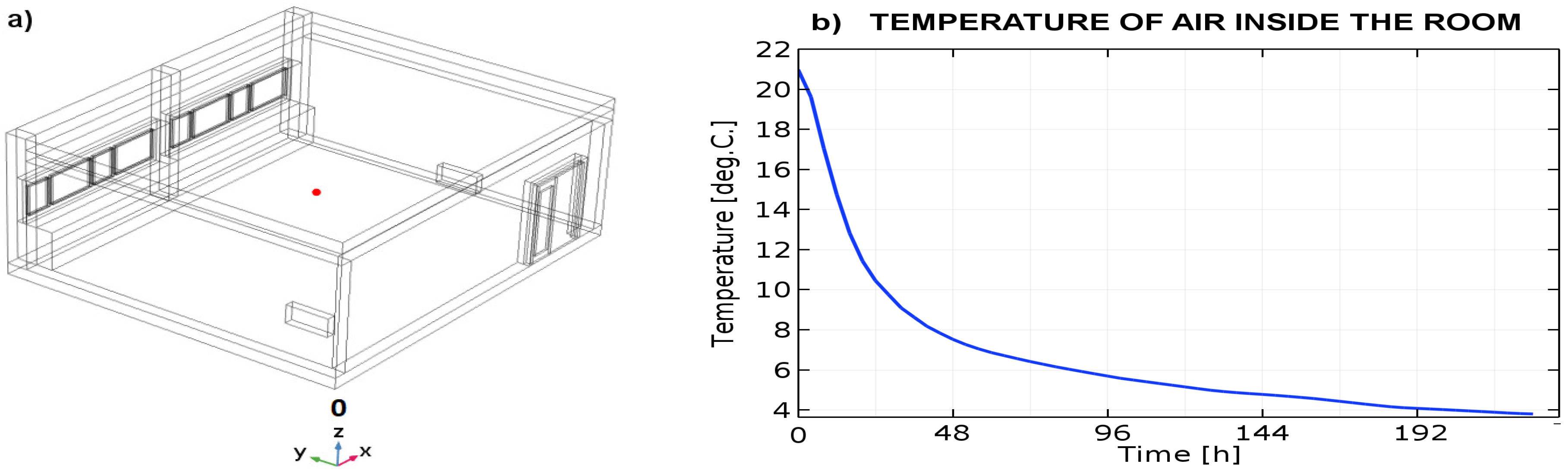
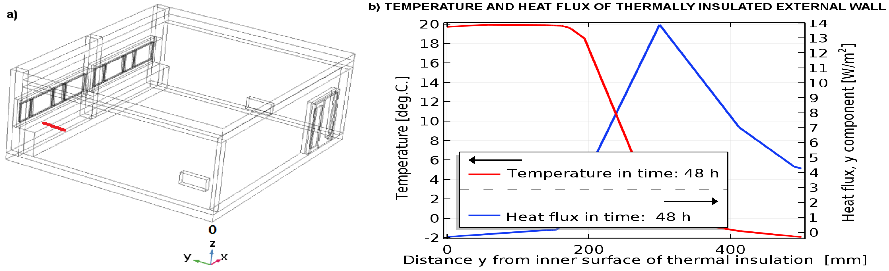
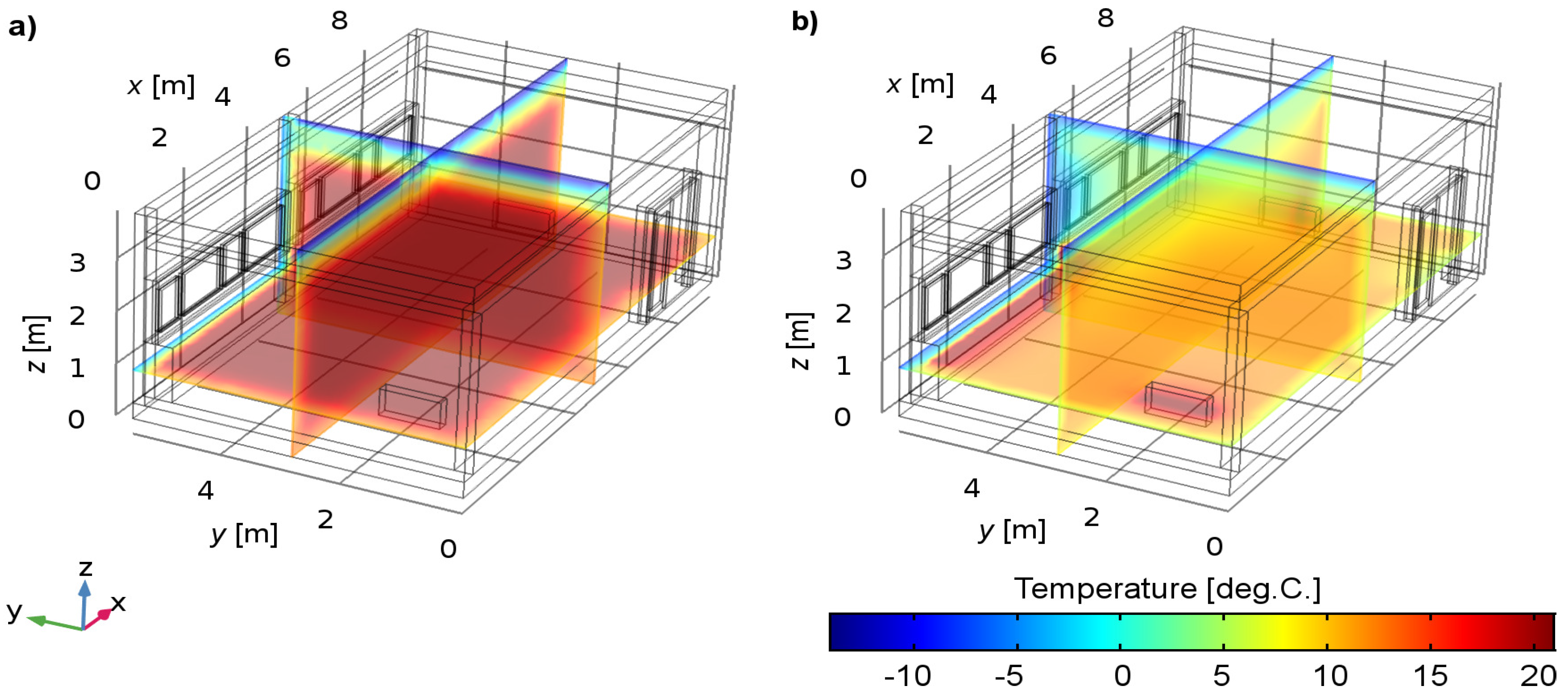
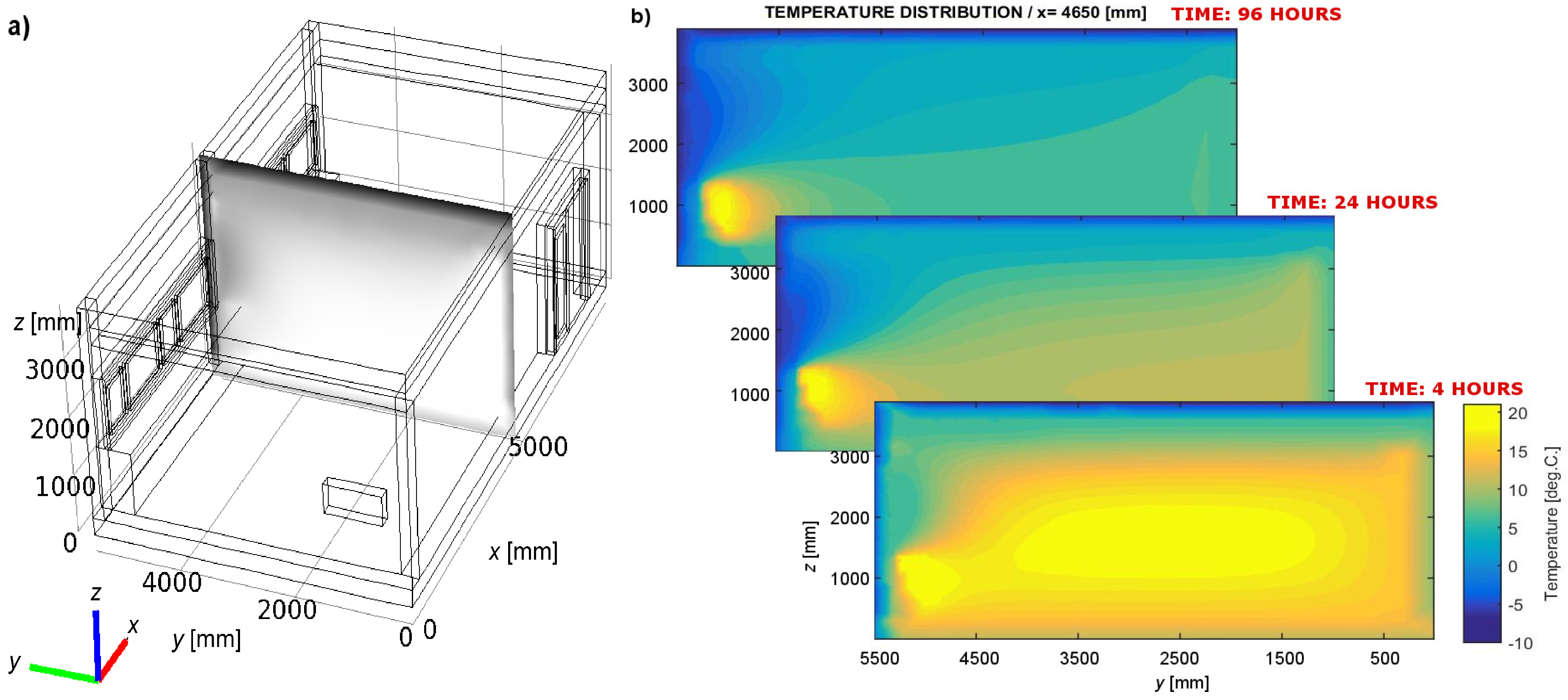
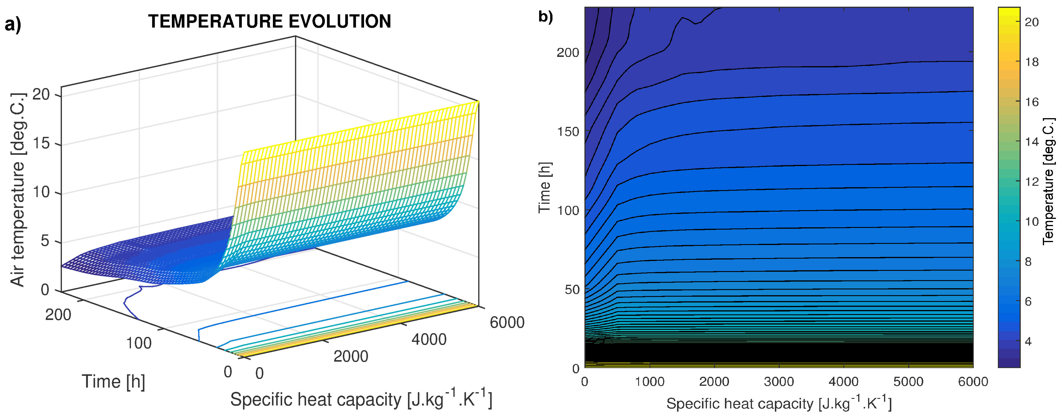
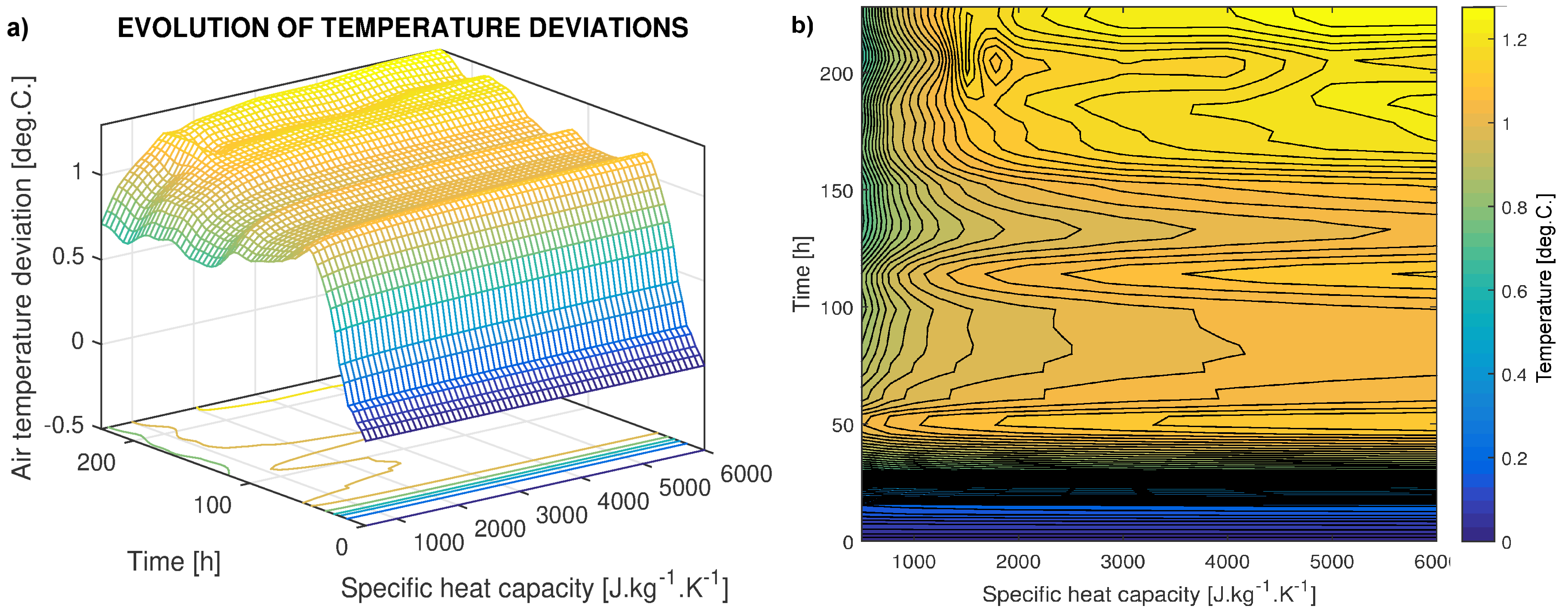
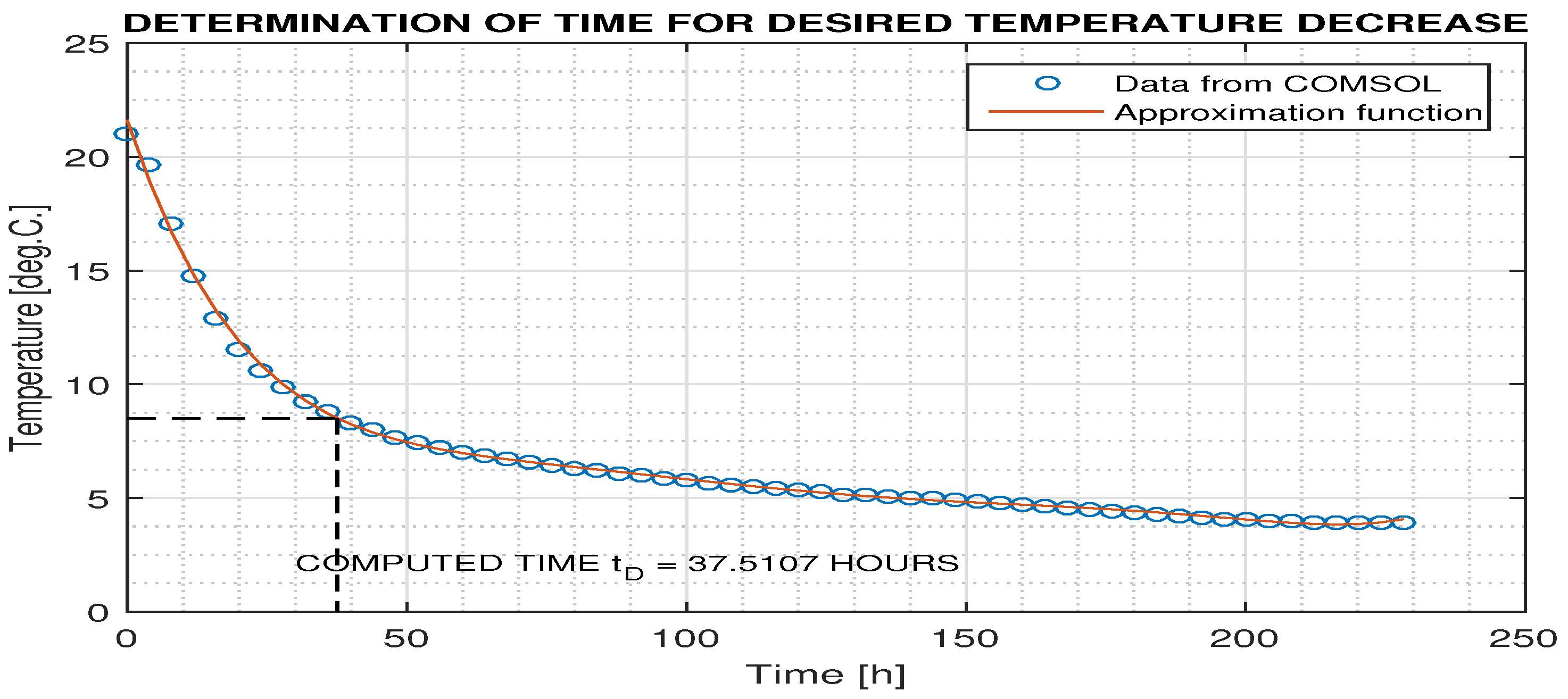
A free tetrahedral mesh specified by a matrix of about 4,200,000 elements (degrees of freedom) was used to solve the finite element problem in the model environment. This matrix includes information about the physics, material property and boundary conditions based on the number of elements and the discretisation order. In this sense, the size of this matrix is closely related to the complexity of the whole problem, demands for the size of computer memory, and time necessary for numerical modelling of the whole spatial model. The meshed model is shown in Figure 3a,b. A blue color indicates an air domain. The used mesh quality was influenced by computer capability. A simple test was performed to determine the air temperature deviation in the study room, dependent on the mesh quality, and to find the optimal mesh density subsequently. The results are shown in Figure 3c. The temperature deviation at the given time of cooling of the room was calculated with regards to the temperature of the model with a minimum element size of 1.49 mm and the maximum element size of 149 mm. These values correspond to the defined size of the model elements and the quality of the finest mesh that could be set with regards to the memory of the computer used. Figure 3c shows an increase of temperature deviation with the increasing maximum and minimum element size (i.e., with decreasing mesh density). For the most coarse meshed model, the maximum temperature deviation is 0.93%, and for the model with the finest mesh, the maximum temperature deviation is 0.57%. With regards to the accuracy of the calculation, the simulation time and the available memory of the used computer, the maximum element size was set to the size of 186 mm. Further choices included the selection of the minimum element size of 1.86 mm, the curvature factor of 0.2, and the maximum element growth rate of 1.3.

The average simulation time took about 110 min for the selected sampling period of 4 h. The model was calculated using COMSOL Multiphysics 5.3 on a computer with the processor Intel(R) Core(TM) i7-8550U CPU 1.80 GHz, 4 cores. The available memory was 16.22 GB. The whole simulation was performed by the PARADISO solver which is a part of the COMSOL Multiphysics software. An absolute tolerance for control of the largest allowable absolute error at any step of simulation was 0.001.

The quadratic Lagrange discretisation method was used for solving of the studied model. Further discretisation methods tested during simulations included linear and quadratic serendipity, Lagrange cubic discretisation, cubic serendipity, Lagrange quartic, quartic serendipity, and Lagrange quintic discretisation. Best results were obtained by the Lagrange quadratic and quadratic serendipity discretisation methods. The size of computer memory and time necessary for numerical modelling were similar for both of these methods. Errors were recorded for linear discretisation under the conditions considered. Too extensive computing time or lack of computer memory were the most restrictive factors for other discretisation methods.

3. Results

The main results of simulations are shown in Figure 4, Figure 5 and Figure 6. Figure 4 shows a decrease of the air temperature in the middle the room as a result of heat transfer to the unheated adjoining rooms and to the environment outside the building. Figure 5 depicts the temperature and heat flux curves through the outside wall after two days of cooling the room. These curves can also be obtained for any other time of cooling by entering the required value of the appropriate box of the computer application. The time evolution of temperature and heat flow provides important information about the wall’s thermal accumulation properties and the time needed to achieve steady heat transfer.

Similarly, Figure 6a shows sections with the distribution of the air temperature inside the room as well as temperatures in the walls. Figure 6a shows initial temperature distribution and Figure 6b shows temperature distribution after one day of cooling. This data can also be obtained for any other time of cooling.

The output data from the simulations using COMSOL Multiphysics were processed with the use of MATLAB software, as shown below. In the presented case, the width of the room is 5 m and the thermal insulation thickness is 400 mm. The supposed temperature everywhere outside the room is $0{}^{°}\mathrm{C}$. The other parameters are the same as in the previous case. The output data from the simulations before processing in MATLAB software is included as Supplements S3, S4.

Figure 7 shows the temperature distributions in the selected section of the room processed in MATLAB as color slices with the desired color resolution. A video sequence of these slices calculated for the cooled room with time steps of four hours forms the temperature evolution, which is shown in Supplement S2.

Figure 8 and Figure 9 depict the temperature of the air inside the cooled room with respect to the specific heat capacity of the outside wall thermal insulation. Figure 8a depicts the time evolution of the air temperature in the middle of the room as a 3D plot. The 2D temperature distribution is shown in Figure 8b. The velocity of cooling the room decreases with increasing specific heat capacity of the thermal insulation of the outside wall, which is reflected by increasing temperature of the air inside the room.

Figure 9 presents deviations of the air temperature while cooling the thermally insulated room from the air temperature in the room with non-insulated outside wall. It is evident that the temperature deviation increases as the thermal insulation capacity of the thermal insulation increases. Under these conditions, the maximum temperature deviation is $1.3{}^{°}\mathrm{C}$ in the room thermally insulated by the material of the specific heat capacity of $6000\mathrm{J}·{\mathrm{kg}}^{-1}·{\mathrm{K}}^{-1}$.

The degree of utilisation of heat gains or thermal heat losses is directly related to the thermal inertia of the building. Based on the inner heat capacity of the building structure, a time to achieve desired temperature decrease can be determined. In the presented example, the desired temperature was computed from the polynomial, which can approximate temperature evolution of the air inside the tested room during its cooling. For this purpose, the output data from the simulations were approximated by polynomial of the 6th degree using the MATLAB software. The applied procedure for computing the described model and conditions is shown in Figure 10.

Table 3. Computed time of the 20 percent temperature decrease. $t_{D200}$ is the cooling time for a 200 mm thick wall insulation, $t_{D300}$ for a 300 mm thick wall insulation, and $t_{D400}$ for a 400 mm thick wall insulation.

${\mathit{c}}_{\mathit{p}}\left[\mathbf{J}·{\mathbf{kg}}^{-1}·{\mathbf{K}}^{-1}\right]$	Room with Windows			Room without Windows
	${\mathit{t}}_{\mathit{D}200}\left[\mathbf{h}\right]$	${\mathit{t}}_{\mathit{D}300}\left[\mathbf{h}\right]$	${\mathit{t}}_{\mathit{D}400}\left[\mathbf{h}\right]$	${\mathit{t}}_{\mathit{D}200}\left[\mathbf{h}\right]$	${\mathit{t}}_{\mathit{D}300}\left[\mathbf{h}\right]$	${\mathit{t}}_{\mathit{D}400}\left[\mathbf{h}\right]$
500	12.6074	13.3499	14.2084	18.1518	22.0157	24.5785
750	12.9352	13.7329	14.4724	19.5924	23.7279	25.8499
1000	13.1871	13.9521	14.6941	20.6716	24.7484	26.4313
1250	13.3796	14.1097	14.7164	21.4888	25.3784	26.7341
1500	13.5251	14.3165	14.8331	22.1175	25.7770	26.9165
1750	13.5287	14.2861	14.9097	22.6085	26.0335	27.0439
2000	13.7390	14.3729	14.9442	22.9967	26.2005	27.1444
3000	13.9666	14.4867	15.2986	23.9202	26.4593	27.4503
4000	13.9131	14.4992	15.3654	24.3236	26.5035	27.6890
5000	13.9715	14.5845	15.4119	24.5015	26.5105	27.8799
6000	14.0064	14.5970	15.4464	24.5761	26.5175	28.0317

and

Table 4. Computed time of the 50 percent temperature decrease. $t_{D200}$ is the cooling time for a 200 mm thick wall insulation, $t_{D300}$ for a 300 mm thick wall insulation, and $t_{D400}$ for a 400 mm thick wall insulation.

${\mathit{c}}_{\mathit{p}}\left[\mathbf{J}·{\mathbf{kg}}^{-1}·{\mathbf{K}}^{-1}\right]$	Room with Windows			Room without Windows
	${\mathit{t}}_{\mathit{D}200}\left[\mathbf{h}\right]$	${\mathit{t}}_{\mathit{D}300}\left[\mathbf{h}\right]$	${\mathit{t}}_{\mathit{D}400}\left[\mathbf{h}\right]$	${\mathit{t}}_{\mathit{D}200}\left[\mathbf{h}\right]$	${\mathit{t}}_{\mathit{D}300}\left[\mathbf{h}\right]$	${\mathit{t}}_{\mathit{D}400}\left[\mathbf{h}\right]$
500	32.1153	33.8433	35.9988	55.1043	80.0684	91.1732
750	32.8130	34.6268	36.7179	63.5432	92.1786	102.1550
1000	33.3046	35.0553	37.2446	70.5980	99.1117	107.5477
1250	33.6671	35.3828	37.3249	76.1967	103.1024	110.2212
1500	33.9439	35.7448	37.5107	80.5065	105.3731	111.5354
1750	34.1608	35.7814	37.6306	83.7865	106.6239	112.1786
2000	34.3339	35.9529	37.9464	86.2689	107.2701	112.5012
3000	34.7661	36.7179	38.8484	91.3301	107.5326	113.0086
4000	34.6406	36.7179	39.0384	91.3301	107.5326	113.0086
5000	34.7647	36.5074	39.1732	92.6092	106.7862	114.1834
6000	34.8449	36.5793	39.2757	92.1753	106.7278	114.8614

show the impact of the specific heat capacity of the thermal insulation on the desired time of the temperature decrease. For testing, the specific heat capacity of the insulation was 500–6000 $\mathrm{J}·{\mathrm{kg}}^{-1}·{\mathrm{K}}^{-1}$. The thermal insulation thickness was 200 mm, 300 mm, and 400 mm. The desired time computed for tested room with windows in the external wall (see Figure 1) was compared with a model of a room with an outside wall without windows, which is completely covered by thermal insulation. In the model of room of windows, an area of windows and the window frames represents 48 percent of the outside wall area. The area of the thermal insulation under the windows represents 35 percent of the outside wall area. The results for desired time of the 20 percent temperature decrease are shown in Table 3. Table 4 shows the results for desired time of the 50 percent temperature decrease. The results for room with windows are presented in the left-hand columns of Table 3 and Table 4, the results for room without windows are shown in the right-hand columns of the tables. In both tables, the results confirm increasing time of the room temperature drop with increasing specific heat capacity and the thickness of the thermal insulation of the outside wall. It is also evident that the windows have a considerable influence on the heat loss of the room. The time to reach the temperature drops by 20 percent was in the room with windows from 1.4 to 1.8 times lower than in the room without windows. The time to reach the temperature drops by 50 percent was in the room with windows from 1.7 to 2.9 times lower than in the room without windows under the studied conditions. The mesh statistic for determination of desired temperature decrease with respect to the geometry of the model and the thickness of the thermal insulation are given in

Table 5. The mesh statistic for determination of desired temperature decrease for a 200 mm ($I_{200}$) thick wall insulation, for a 300 mm ($I_{300}$) thick wall insulation, and for a 200 mm ($I_{400}$) thick wall insulation. The numbers given indicate the number of elements.

Description	Room with Windows			Room without Windows
	${\mathit{I}}_{200}$	${\mathit{I}}_{300}$	${\mathit{I}}_{400}$	${\mathit{I}}_{200}$	${\mathit{I}}_{300}$	${\mathit{I}}_{400}$
Minimum element quality	0.01214	0.01214	0.01214	0.09427	0.09427	0.09427
Average element quality	0.7235	0.7239	0.7237	0.7716	0.7738	0.7710
Tetrahedral elements	3,062,131	3,058,890	3,062,773	519,500	512,976	519,485
Triangular elements	378,689	378,706	378,558	45,982	46,160	46,048
Edge elements	12,220	12,203	12,184	2611	2615	2611
Vertex elements	276	276	276	112	112	112

.

4. Discussion

Heat accumulation properties of building structures’ materials significantly affect the cost of heating or cooling of buildings. In practice, the energy performance of buildings is assessed, in particular by theoretical calculations based on valid technical standards for construction and architecture.

However, these standards are often very demanding and, moreover, they consider many simplifications compared to real conditions, which can significantly affect the accuracy of the results obtained. In contrast, the use of suitable software tools for modelling physical processes is an important advantage, the possibility to perform simulations for marginal conditions inserted in the form of data obtained by real measurement on the object under consideration. However, for objective assessment of the thermal properties of buildings, the output data from computer simulations should be subsequently processed by the uniform methodical procedures of the technical calculations generally used in engineering practice. Therefore, research is focused on testing the factors that influence the thermal stability of a building. We have used a combination of computer simulations in the COMSOL Multiphysics user interface and theoretical calculations using the European technical standards for the building industry.

This paper presents a study of the thermal stability of the model with various geometry sizes and material properties of all elements of the room. Compared to the previously published models of a heated (cooled) room [32,34], the thermal insulation of the outer wall is now incorporated into the model, which allows its much wider use by testing of thermal distribution inside the studied room and searching for the optimal thermal insulation material properties. Additionally, the graphical user interface created with Application Builder provides engineers and scientists the opportunity to use the model without necessarily having knowledge of COMSOL Multiphysics control. Accuracy of the basic model that was used for transformation into the computer application was verified by experimental testing [32].

The current results are presented in Figure 7, Figure 8, Figure 9 and Figure 10 and in Supplement S2. The mesh density analysis was performed by comparing the air temperature evolution in the model of the selected mesh quality and in the model with the maximum mesh density that could be set with regards to available memory of the used computer. The maximum temperature deviation calculated for the mesh of the presented model was 0.57%. The mean and median error values were 0.08% and 0.04%, respectively.

5. Conclusions

The present results form the basis for more complex simulations of thermal properties inside newly designed buildings. The heat transfer incorporated into the assembled model will be enriched by information related to moisture transfer and various types of heating as well. The future work will be devoted to the subsequent processing of output data obtained by computer simulations to determine the additional criteria and parameters that are used to assess the heat losses of buildings. This information will enable a more detailed balance of energy to optimize its requirements for building heating (cooling) or architectural changes that can eliminate thermal losses of buildings under given conditions. In this respect, the MATLAB computational tools will be used to analyse the temperature evolution in the room. The influence of permanent or cyclic heating of the room by modifying the boundary conditions will be studied as well.

It is assumed that the future work will include studies related to visualization in engineering [39], modelling of temperature distribution both inside the room and in the walls [30,32,34], and the study of comfortable indoor environment to keep emotional and physical states of individuals healthy [40]. Simulations or thermal imaging [39] for breathing analysis using thermal and depth imaging camera video records will be included in the future research too.

References

1. Zawieska, J.; Pieriegud, J. Smart city as a tool for sustainable mobility and transport decarbonisation. Transp. Policy 2018, 63, 39–50. [Google Scholar] [CrossRef]
2. Lazaroiu, G.C.; Mariacristina, R. Definition methodology for the smart cities model. Energy 2012, 47, 326–332. [Google Scholar] [CrossRef]
3. De Groote, M.; Fabbri, M. Smart Buildings in a Decarbonised Energy System; Buildings Performance Institute Europe (BPIE): Brussels, Belgium, 2016. [Google Scholar]
4. Kejriwal, S.; Mahajan, S. Smart Buildings. How IoT Technology Aims to Add Value for Commercial Real Estate Companies. Available online: https://www2.deloitte.com/insights/us/en/focus/internet-of-things/iot-commercial-real-estate-intelligent-building-systems.html (accessed on 16 November 2018).
5. Weng, T.; Agarval, Y. From buildings to smart buildings—Sensing and actuation to improve energy efficiency. IEEE Des. Test Comput. 2012, 29, 36–44. [Google Scholar] [CrossRef]
6. Battista, G.; Evangelisti, L.; Guattari, C.; Basilicata, C.; de Lieto Vollaro, R. Buildings energy efficiency: Interventions analysis under a smart cities approach. Sustainability 2014, 6, 4694–4705. [Google Scholar] [CrossRef]
7. Heim, D.; Wieprzkowicz, A. Attenuation of temperature fluctuations on an external surface of the wall by a phase change material-activated layer. Appl. Sci. 2018, 8. [Google Scholar] [CrossRef]
8. Shen, C.; Li, X. Potential of Utilizing Different Natural Cooling Sources to Reduce the Building Cooling Load and Cooling Energy Consumption: A Case Study in Urumqi. Energies 2017, 10, 366. [Google Scholar] [CrossRef]
9. Bisegna, F.; Mattoni, B.; Gori, P.; Asdrubali, F.; Gyatarri, C.; Evangelisti, L.; Sambuco, S.; Bianchi, F. Influence of insulating materials on green building rating system results. Energies 2016, 9, 712. [Google Scholar] [CrossRef]
10. Li, M.; Gui, G.; Lin, Z.; Jiang, L.; Pan, H.; Wang, X. Numerical thermal characterization and performance metrics of building envelopes containing phase change materials for energy-efficient buildings results. Sustainability 2018, 10, 2657. [Google Scholar] [CrossRef]
11. Ferroukhi, M.; Belarbi, R.; Limam, K.; Bosschaerts, W. Impact of coupled heat and moisture transfer effects on buildings energy consumption. Therm. Sci. 2017, 21, 1359–1368. [Google Scholar] [CrossRef]
12. Badea, N. Design for Micro-Combined Cooling, Heating and Power Systems: Stirling Engines and Renewable Power Systems; Springer-Verlag: London, UK, 2015. [Google Scholar]
13. Zmrhal, V.; Hensen, J.L.M.; Drkal, F. Modeling and simulation of a room with a radiant cooling ceiling. In Proceedings of the 8th International IBPSA Building Simulation Conference, Eindhoven, The Netherlands, 11–14 August 2003; pp. 1491–1496. [Google Scholar]
14. Tam, W.; Yuen, W.; Chow, W. Numerical study on the importance of radiative heat transfer in building energy simulation. Numer. Heat Transf. Part A Appl. 2016, 69, 694–709. [Google Scholar] [CrossRef]
15. Rodriguez-Munoz, N.A.; Najera-Trejo, M.; Alarcon-Herrera, O.; Martin-Dominguez, I.R. A building’s thermal assessment using dynamic simulation. Indoor Built Environ. 2018, 27, 173–183. [Google Scholar] [CrossRef]
16. Perera, D.W.U.; Skeie, N.-O. Estimation of the Heating Time of Small-Scale Buildings Using Dynamic Models. Buildings 2016, 6, 10. [Google Scholar] [CrossRef]
17. Bahar, Y.N.; Pere, Ch.; Landrieu, J.; Nicolle, C. A Thermal Simulation Tool for Building and Its Interoperability through the Building Information Modeling (BIM) Platform. Buildings 2013, 3, 380–398. [Google Scholar] [CrossRef][Green Version]
18. Taoum, S.; Lefrançois, E. Dual analysis for heat exchange: Application to thermal bridges. Comput. Math. Appl. 2018, 75, 3471–3487. [Google Scholar] [CrossRef]
19. Sehnalek, S.; Zalesak, M.; Vincenec, J.; Oplustil, M.; Chrobak, P. Evaluation of SolidWorks Flow Simulation by Ground-Coupled Heat Transfer Test Cases. In Proceedings of the International Conferences: Latest Trends on Systems, Latest Trends on Systems, Santorini, Greece, 17–21 July 2014; Volume II, pp. 492–498. [Google Scholar]
20. Maliki, M.; Laredj, N.; Bendani, K.; Missoum, H. Two-dimensional transient modeling of energy and mass transfer in porous building components using COMSOL Multiphysics. J. Appl. Fluid Mech. 2017, 10, 319–328. [Google Scholar] [CrossRef]
21. Promis, G.; Douzane, O.; Tran Le, A.D.; Langlet, T. Moisture hysteresis influence on mass transfer through bio-based building materials in dynamic state. Energy Build. 2018, 166, 450–459. [Google Scholar] [CrossRef]
22. Kupczak, A.; Sadłowska-Sałęga, A.; Krzemień, L.; Sobczyk, J.; Radoń, J.; Kozłowski, R. Impact of paper and wooden collections on humidity stability and energy consumption in museums and libraries. Energy Build. 2018, 158, 77–85. [Google Scholar] [CrossRef]
23. Portal, N.; van Schijndel, A.; Kalagasidis, A. The multiphysics modeling of heat and moisture induced stress and strain of historic building materials and artefacts. Build. Simul. 2014, 7, 217–227. [Google Scholar] [CrossRef]
24. Bida, S.M.; Aziz, F.N.A.A.; Jaafar, M.S.; Hejazi, F.; Nabilah, A.B. Thermal performance of super-insulated precast concrete structural sandwich panels. Energy Build. 2018, 176, 418–430. [Google Scholar] [CrossRef]
25. Tsvetkov, N.; Khutornoi, A.; Kozlobrodov, A.; Romanenko, S.; Shefer, Y.; Golovko, A. Influence of metal frame on heat protection properties of a polystyrene concrete wall. MATEC Web Conf. 2018, 143, 1–7. [Google Scholar] [CrossRef]
26. Bianchi Janetti, M.; Colombo, L.P.M.; Ochs, F.; Feist, W. Effect of evaporation cooling on drying capillary active building materials. Energy Build. 2018, in press. [Google Scholar] [CrossRef]
27. Putra, J. A Study of Thermal Comfort and Occupant Satisfaction in Office Room. Procedia Eng. 2017, 170, 240–247. [Google Scholar] [CrossRef]
28. Missoum, A.; Elmir, M.; Bouanini, M.; Draoui, B. Numerical simulation of heat transfer through the building facades of buildings located in the city of Bechar. Int. J. Multiphys. 2016, 10, 441–450. [Google Scholar]
29. Biswas, K. Development and Validation of Numerical Models for Evaluation of Foam-Vacuum Insulation Panel Composite Boards, Including Edge Effects. Energies 2018, 11, 2228. [Google Scholar] [CrossRef]
30. Gerlich, V.; Sulovská, K.; Zálešák, M. COMSOL Multiphysics validation as simulation software for heat transfer calculation in buildings: Building simulation software validation. Meas. J. Int. Meas. Confed. 2013, 46, 2003–2012. [Google Scholar] [CrossRef][Green Version]
31. Neymark, J.; Judkoff, R. International Energy Agency Building Energy Simulation TEST and Diagnostic Method (IEA BESTEST). In Depth Diagnostic Cases for Ground Coupled Heat Transfer Related to Slab-on-Grade Construction; National Renewable Energy Lab.: Golden, CO, USA, 2008. [Google Scholar]
32. Charvátová, H.; Zálešák, M. Calculation of heat losses of the room with regard to variable outside air temperature. In Proceedings of the 19th International Conference on Systems, Recent Advances in Systems, Zakynthos Island, Greece, 16–20 July 2015; pp. 627–631. [Google Scholar]
33. Eppes, T.; Milanovic, I. Application building in engineering courses. In Proceedings of the Global Engineering Education Conference (EDUCON), Athens, Greece, 25–28 April 2017; pp. 78–85. [Google Scholar]
34. Charvátová, H.; Zálešák, M. Testing of Method for Assessing of Room Thermal Stability. MATEC Web Conf. 2017, 125. [Google Scholar] [CrossRef]
35. CSN EN ISO 13790: Energy Performance of Buildings—Calculation of Energy Consumption for Heating and Cooling, (Czech Edition) ed; Czech Office for Standards, Metrology and Testing: Prague, Czech Republic, 2009.
36. COMSOL Multiphysics 5.3; COMSOL, Inc.: Stockholm, Sweden, 2017.
37. Nikishkov, G.P. Introduction to the Finite Element Method. Lecture Notes; University of Aizu: Aizu-Wakamatsu, Japan, 2004. [Google Scholar]
38. Carslaw, H.S.; Jaeger, J.C. Conduction of Heat in Solids; Clarendon Press: Oxford, UK, 1986. [Google Scholar]
39. Procházka, A.; Charvátová, H.; Vyšata, O.; Kopal, J.; Chambers, J. Breathing Analysis Using Thermal and Depth Imaging Camera Video Records. Sensors 2017, 17, 1408. [Google Scholar] [CrossRef] [PubMed]
40. Spilak, M.P.; Sigsgaard, T.; Takai, H.; Zhang, G. A comparison between temperature-controlled laminar airflow device and a room air-cleaner in reducing exposure to particles while asleep. PLoS ONE 2016, 11, e0166882. [Google Scholar] [CrossRef] [PubMed]
Figure 1. Geometric layout of the studied model.
Energies 11 03205 g001
Figure 2. Temperatures of air in the adjoining rooms and the temperature of the air outside the building—data used as the boundary conditions for the tested model.
Energies 11 03205 g002
Figure 3. Meshed model: (a) sketch of the model; (b) close-up view of a section near the outer wall; and (c) percentage temperature deviations related to the mesh densities.
Energies 11 03205 g003
Figure 4. Time evolution of the air temperature in the center of the room: (a) sketch of the monitored location (the red point) inside the room; (b) dependence of the air temperature on time of cooling the room.
Energies 11 03205 g004
Figure 5. Temperature and heat flow in the outside wall after two days of cooling the room: (a) position of the monitored place (the red line); (b) temperature and heat flow distribution.
Energies 11 03205 g005
Figure 6. Slices of temperature inside the cooled room: (a) initial temperature distribution; (b) temperature distribution after one day of cooling.
Energies 11 03205 g006
Figure 7. Distribution of the air temperature in selected times of cooling the room: (a) the spatial location of the plane in which the temperature was determined; (b) slices with the temperature distributions.
Energies 11 03205 g007
Figure 8. Time evolution of the air temperature in the middle of the room concerning the specific heat capacity of the outside wall thermal insulation as (a) 3D plot and (b) 2D temperature distribution.
Energies 11 03205 g008
Figure 9. Deviation of the air temperature while cooling the thermally insulated room from the room with non-insulated outside wall as (a) 3D plot and (b) 2D temperature distribution.
Energies 11 03205 g009
Figure 10. Determination of desired temperature decrease from time evolution of the air temperature inside the cooled room based on approximation of output data from COMSOL Multiphysics by polynomial of the 6th degree.
Energies 11 03205 g010