Modelling the Dynamics of Fuel and EU Allowance Prices during Phase 3 of the EU ETS

Abstract

This article studies the relationship between the prices of fuel and EU Allowances (EUA) for carbon emissions during Phase 3 of the European Union Emissions Trading System. We find that the forward prices of EUA, coal, gas and Brent oil are jointly determined in equilibrium. The existence of such a long-run relationship entails a permanent-transitory decomposition for the series of EUA and fuel prices that reveals the short- and long-term causal influence of the EUA market in shaping the joint dynamics of fuel prices. This result complements the literature that suggests that EUA prices are driven by the dynamics of fuel prices. Interestingly, we do not find an equilibrium relationship in the spot market. EUA and fuel spot prices are driven by independent unit root processes. The differences between spot and forward markets are attributed to the tradability of forward prices that are used for speculation and hedging in financial markets. In contrast, spot prices are mainly driven by supply and demand in energy markets.

1. Introduction

The European Union Emissions Trading System (EU ETS) is a key tool for reducing greenhouse gas emissions and the world’s first and biggest carbon market. It works on the ‘cap and trade’ principle. Within the cap, which is set on the total amount of greenhouse gasses that can be emitted, companies receive or buy emission allowances that can be traded. At the moment, the EU ETS is in Phase 3 (2013–2020), which is significantly different from Phases 1 (2005–2007) and 2 (2008–2012). It operates in 31 countries (the 28 EU States, Iceland, Liechtenstein and Norway) and covers approximately 11,000 power plants and manufacturing installations (power stations, oil refineries, production of iron, aluminium, cement, lime, glass, ceramics, etc.), as well as approximately 520 airlines flying in Europe. It also covers around $45\%$ of the EU’s greenhouse gas emissions. We refer to Goulder and Parry [1], Aldy and Stavins [2] and Baranzini et al. [3] for a deep discussion on carbon pricing policies and to Aldy and Stavins [2] and Ellerman et al. [4] for a review on the EU ETS performance during the last few years.

Participants in the EU ETS can use international credits, such as emission reduction units (ERUs) and certified emission reductions (CERs) in order to fulfil part of their obligations, subject to qualitative and quantitative restrictions. CERs and ERUs are obtained by investing in projects that reduce emissions in developing countries; see, for example, Gronwald and Hintermann [5] for a model relating EU Allowances (EUA) and CER. However, since Phase 3, these international credits are no longer compliance units and must be exchanged for EU allowances. By 30 April of each year, installations must surrender an EUA for each ton of CO₂ emitted in the previous year. During Phase 1, most allowances in all countries were given freely (known as grandfathering). However, during Phase 3, $57\%$ of the total amount of allowances will be auctioned. In principle, anyone can trade in the carbon market, but the main traders are energy companies, industrial companies and financial intermediaries such as banks.

How the EUA price is determined is of great interest for policy makers, but also for all market participants. There is a consensus in the literature about pointing out that allowance prices are significantly related to fuel prices and to variables such as economic activity or changes in the cap. However, the empirical evidence on the specific form of this relationship is inconclusive and not robust to the specification of the model and the time period under study, see, for example, Zhang [6] and Hintermann et al. [7] for a detailed review of the literature during the previous phases of the EU ETS. Furthermore, most of the econometric models used in the empirical literature for describing the dynamics of EU allowances focus on log-returns and not on the series of prices and, hence, cannot obtain meaningful conclusions on the relation between EUA and fuel prices. The aim of this paper is to uncover the presence of a long-run relationship between these series that drives the dynamics of EUA emissions in equilibrium during Phase 3 of the EU ETS market. To do this, we apply a vector autoregressive process (VAR) between the prices of oil, coal, gas and EU allowances. This setting allows us to interpret the four time series of prices as endogenously determined. Although there are some articles that already consider EUA prices as an endogenous variable (see, for example, Bredin and Muckley [8], Creti et al. [9] and Rickels et al. [10]), this view is rather unexplored in the literature, which usually considers fuel prices as exogenous determinants of EUA prices. We focus on the price of coal, gas and Brent oil. Coal and gas are the main commodities for generating energy and are also the main polluting fuels. Their consumption is associated with the acquisition of licences to pollute in the form of EU carbon emission allowances. For completeness, we also consider Brent crude oil as another fuel widely used for generating energy, but also as a proxy of economic activity. In contrast to some recent literature, we do not consider energy consumption variables. This decision is based on the work of Jaforullah and King [11] who argued that the presence of energy consumption variables in a model of carbon emissions can lead to misleading cointegration test results.

The contributions of this article to the literature on the relationship between fuel prices and carbon emissions are three-fold. First, we find that EUA forward prices are jointly determined along with fuel forward prices during Phase 3 of the EU ETS. The existence of a long-run relationship entails the presence of common trends that drive the permanent component of fuel prices and EUA in the forward market. Forward prices are traded in financial markets and governed, in turn, by market forces that prevent the presence of arbitrage opportunities. These market forces impose the existence of joint dynamics in forward prices and, more specifically, the presence of an equilibrium relationship. The Vector Error Correction Model (VECM) representation of the multivariate time series of EUA and fuel prices also allows us to model the dynamics of the corresponding financial returns. In particular, we find empirical evidence of the predictive ability of the error correction component on the returns on EUA, coal, gas and Brent oil prices.

Our second contribution is to show that the existence of such long-run equilibrium relationship between EUA and fuel prices is not present in the spot market. Investors hedge and speculate in forward markets, but not in the spot market; hence, spot prices are not governed by market forces and no-arbitrage conditions to the same extent as forward prices. More specifically, we find that spot prices of EUA, gas, coal and Brent oil are not cointegrated and, therefore, do not share common trends. Their dynamics obey idiosyncratic forces determined by demand and supply in equilibrium.

Our third contribution is to exploit the existence of a long-run equilibrium relationship between EUA, coal, gas and Brent oil forward markets that allows us to apply the Gonzalo and Granger [12] permanent-transitory decomposition for the time series of EUA and fuel prices. To the best of our knowledge, this type of analysis (the use of price discovery techniques based on cointegration and a permanent-transitory decomposition) to determine the common drivers of EUA and fuel prices in the forward market has not been done in the empirical literature concerned with the market for carbon emissions, at least for Phase 3. Our empirical results obtained over the period January 2013–May 2017 uncover the existence of common trends driving the joint dynamics of these series. In this analysis, we observe the important influence of the EUA market in shaping the joint dynamics of the time series. In fact, including EUA prices in the vector of fuel prices improves the fit of the time series of coal and gas at daily and weekly frequencies, but not at monthly frequencies.

The rest of the paper is organised as follows. Section 2 reviews empirical research on the topic and summarizes the main results found in the literature. Section 3 contains the results of the cointegration analysis and discusses the equilibrium dynamics between fuel and EUA prices at daily, weekly and monthly frequencies. The permanent-transitory decomposition of Gonzalo–Granger is discussed in Section 4. Finally, Section 5 concludes the paper with a summary of the main results and proposals for further research.

2. Literature Review

How EU allowances and fuel prices relate is an open question that has attracted the interest of researchers since the beginning of the EU ETS in 2005. The literature has addressed the problem by looking at different data from Phases 1 and 2, but also by using different econometric methods, which can explain in part the different and, sometimes, contradictory results. The econometric methods used depend on whether the data analysed are stationary (returns) or not (prices). In this sense, some papers use regression methods to model the returns, while others rely on cointegration methods trying to model the long-run relationship of the price series. Furthermore, there are also important differences in the data analysed. Some studies look at spot prices, while others consider forward prices; there are also differences depending on the type of fuels analysed and the frequency of the data.

The work of Alberola et al. in [13] is one of the papers dealing with time series of returns. These authors used daily data from Phase 1 considering spot prices of EUA and one-month ahead forward prices of coal, gas and Brent oil. They focused on the empirical relationship between EUA returns and their main fundamentals using regression models. Hintermann [14] used daily spot and forward prices of EUA, coal and gas also observed during Phase 1. The estimated models, using return series, include also data on temperature, precipitation and Nordic reservoir levels. This author assumed that spot and futures prices are equal except for a possible difference caused by storage costs. His results differ depending on the estimated regression model. Chevallier [15] investigated the impact of fuel use (Brent oil, gas and coal) on carbon prices using one-month-ahead forward prices observed from 2007–2009 (data from both Phases 1 and 2) and regression methods applied to the series of returns. Lutz et al. [16] used daily forward prices of EUA, coal, gas and Brent oil observed during Phase 2. To control for the macroeconomic conditions, their models also included the Dow Jones Euro Stoxx 50, the Thomson Reuters/Jeffries Commodity Research Bureau Index (CRBI), as an indicator capturing risk related to fluctuations of global commodity markets, and a default spread series to account for default risks in credit markets. They also considered time series of temperatures and estimated a Markov regime switching GARCH model, accounting for changing states in the mean and variance of the EUA returns.

One of the main problems of using regression models to explain the returns of the EUA as a function of the fuel returns is the underlying assumption that coal, gas and Brent prices are exogenous variables influencing EUA prices instead of considering the possibility that all four prices are determined jointly. In this sense, Aatola et al. [17] also modelled the series of returns, by using daily forward prices of EUA observed from 2005–2010, but they considered several econometric models with multiple stationary time series, such as VAR models, to allow all the variables to be endogenous. They argued that there is a strong relationship between the fundamentals, such as German electricity prices and gas and coal prices, and the EUA price.

All previous papers looked at the sign and statistical significance of the corresponding coefficients of the models in order to uncover the relationship between the EUA and fuel prices, and all of them agreed in finding a positive and significant relationship between the prices of EUA and gas. When looking at the relationship between the prices of EUA and Brent oil, Alberola et al. [13] found it not significant, while Chevallier [15] found it positive and significant at the 10% level. The main differences appear when looking at the relationship between the prices of EUA and coal. It is found to be negative and significant in Alberola et al. [13], Chevallier [15] and Aatola et al. [17], positive although not significant in Hintermann [14] and positive and statistically significant in Lutz et al. [16].

Being aware of the problems of assuming the EUA price formation in terms of a set of exogenous determinants, an alternative line of research has focused on modelling the time series of prices. The work of Fezzi and Bunn in [18] is one of the first papers using cointegration methods. They used daily spot prices of EUA, gas and electricity in the U.K. observed from 2005–2006 (Phase 1) and found a cointegration relationship between those series. In contrast, Hintermann [14], using also prices observed during Phase 1, found no cointegration between fuel prices and the EUA price. Bredin and Muckley [8] used daily futures prices of EUA, clean dark and spark energy spreads, Eurex Dow Jones EURO STOXX futures contracts, absolute deviations from mean temperatures and production, as well as futures contracts on oil fossil fuel prices observed from 2005–2009 (data from both Phases 1 and 2). They showed that the series of prices are cointegrated only in Phase 2. Creti et al. [9] used daily forward prices of EUA, coal, gas and Brent oil observed from 2005–2010 (data from both Phases 1 and 2). Their models did not include the prices of coal and gas as two different variables, but the series of switching prices as a proxy of the abatement opportunities. These authors also considered the Dow Jones Euro Stoxx 50 as an equity futures index to proxy the economic conditions. They showed that a cointegrating relationship exists between the prices of EUA, Brent oil, Eurex and the switching price.

With respect to the sign and statistical significance of the corresponding coefficients capturing the long-run relationship between the EUA and fuel prices, Bredin and Muckley [8] found that the long-term relationship between the prices of EUA and gas and Brent oil estimated during Phase 2 was positive and significant. This is in line with the results obtained by Creti et al. [9] using data from both Phases 1 and 2. On the other hand, the long-run relationship between the prices of EUA and coal was estimated as negative and significant in Bredin and Muckley [8], while according to Creti et al. [9], the long-run relationship between the prices of EUA and the switching price was estimated as positive, but only significant in Phase 2.

Rickels et al. [10] used daily forward prices of EUA and different forward prices of coal and gas observed during Phase 2 of the EU ETS. As in Creti et al. [9], some specifications of the models included the series of switching prices and also the Dow Jones Euro Stoxx 50, as well as the price of Brent oil. They found that the existence of cointegration relationships depends on the series of prices included. Their results cannot confirm those in Creti et al. [9], since no cointegration relationship was found when the switching price was included. They argued that in most empirical applications, only one series of coal (gas) prices is chosen. However, there is a large number of coal (gas) prices, for example at different maturities, trading places and places of origin. By estimating auxiliary regression models, these authors showed that different fuel price series have very different explanatory power for EUA prices. They pointed out that this could explain the mixed empirical results on the impact of fuel prices. Their analysis of cointegration relationships delivered mixed results. They showed that cointegration relationships exist, but depend strongly on the fuel price series selected (e.g., gas prices for delivery to United Kingdom vs. delivery to Germany).

There are many other papers analysing either series of returns or prices; however, we have chosen the ones above as good examples to summarize the empirical results found in the literature. More complete reviews of the literature can be found in Zhang [6] and Zhang and Wei [19] for Phase 1 and Hintermann et al. [7] for Phase 2.

3. Equilibrium Dynamics

In this section, we analyse empirically the relationship between the price of EU allowances traded during Phase 3 of the EU ETS and fuel prices. In particular, we are interested in coal, gas and Brent oil prices.

3.1. Data Description

Our sample covers data from 1 January 2013–9 May 2017. For the EUA, we consider spot and futures prices (with maturity in December of the following year) traded on the Intercontinental Exchange Futures Europe (ICE) in London. The construction of the one-year forward price series of EUA is non-standard due to the characteristics of the market for emission allowances. To obtain a meaningful price, we have used the price of the futures contracts with maturity in December 2014, 2015, 2016, 2017 and 2018. Our forward price series is constructed in a similar way to Rickels et al. [10]; however, these authors used the rolling future price series with maturity at the end of the current year, and we use the rolling future price series with maturity at the end of the following year. For example, on 23 January 2014, the price of the one-year forward contract was $5.29$ Euros, which corresponds to the price of the future contract with maturity in December 2015, while the price of the future contract with maturity in December 2014 was $5.10$ Euros. The reason for using this particular series is for consistency with the maturities of the forward price series of coal, gas and Brent oil, which we describe next.

For coal, we use spot and one-year forward price series of API2, a thermal coal shipped from Colombia, Russia, South Africa, Poland, Australia or the U.S. to the Northwest European trading hub of Amsterdam, Rotterdam and Antwerp. The net calorific value (heating value) of this coal in kilocalories per kilogram is 6000. The price is in U.S. dollars per ton. For the gas, we use the series of spot and one-year forward prices of natural gas at the Title Transfer Facility (TTF) Virtual Trading Point, operated by Gasunie Transport Services (GTS), the transmission system operator in the Netherlands. The price is in Euros per MWh. Finally, for oil prices, we use spot and one-year forward prices of Brent. The price is in U.S. dollars per barrel.

3.2. Dynamics of Spot and Forward Prices

We are interested in three different types of dynamic relationships between the price variables. First, we analyse the spot prices of the four series under investigation. Second, we study the long-run dynamics between forward prices at different maturities. Finally, we assess empirically the long-run relationship between spot and forward prices for each of the four time series.

The analysis at the top of

Table 1. (MacKinnon) p-values corresponding to Augmented Dickey–Fuller (ADF) and Phillips–Perron (P-P) unit root tests (left columns) and corresponding to Engle–Granger and Johansen cointegration tests (right columns) for the daily spot (top panel) and forward series (bottom panel).

	Spot Prices
Lags	$\begin{array}{c}\mathbf{ADF}\mathbf{and}\mathbf{Phillips}\text{–}\mathbf{Perron}\\ H_0:\mathrm{unit}\mathrm{root}\end{array}$					$\begin{array}{c}\mathbf{Engle}\text{–}\mathbf{Granger}\\ H_0:\mathrm{no}\mathrm{coint}\end{array}$	$\begin{array}{c}\mathbf{Johansen}\\ H_0:\mathrm{rank}=0\end{array}$
		EUA	Coal	Gas	Oil	p-value	p-value	Log-Lik
1	$\begin{array}{c}ADF\\ P-P\end{array}$	$\begin{array}{c}0.09\\ 0.09\end{array}$	$\begin{array}{c}0.50\\ 0.52\end{array}$	$\begin{array}{c}0.45\\ 0.42\end{array}$	$\begin{array}{c}0.74\\ 0.74\end{array}$	$0.20$	$0.19$	10,660.9
2	$\begin{array}{c}ADF\\ P-P\end{array}$	$\begin{array}{c}0.20\\ 0.12\end{array}$	$\begin{array}{c}0.52\\ 0.52\end{array}$	$\begin{array}{c}0.46\\ 0.44\end{array}$	$\begin{array}{c}0.74\\ 0.74\end{array}$	$0.44$	$0.17$	10,678.4
3	$\begin{array}{c}ADF\\ P-P\end{array}$	$\begin{array}{c}0.24\\ 0.14\end{array}$	$\begin{array}{c}0.49\\ 0.51\end{array}$	$\begin{array}{c}0.50\\ 0.46\end{array}$	$\begin{array}{c}0.73\\ 0.73\end{array}$	$0.52$	$0.34$	10,690.4
4	$\begin{array}{c}ADF\\ P-P\end{array}$	$\begin{array}{c}0.15\\ 0.14\end{array}$	$\begin{array}{c}0.51\\ 0.51\end{array}$	$\begin{array}{c}0.46\\ 0.46\end{array}$	$\begin{array}{c}0.73\\ 0.73\end{array}$	$0.34$	$0.37$	10,695.6
5	$\begin{array}{c}ADF\\ P-P\end{array}$	$\begin{array}{c}0.11\\ 0.13\end{array}$	$\begin{array}{c}0.52\\ 0.51\end{array}$	$\begin{array}{c}0.44\\ 0.46\end{array}$	$\begin{array}{c}0.72\\ 0.73\end{array}$	$0.28$	$0.32$	10,698.9
	Forward Prices
Lags	$\begin{array}{c}\mathbf{ADF}\mathbf{and}\mathbf{Phillips}\text{–}\mathbf{Perron}\\ H_0:\mathrm{unit}\mathrm{root}\end{array}$					$\begin{array}{c}\mathbf{Engle}\text{–}\mathbf{Granger}\\ H_0:\mathrm{no}\mathrm{coint}\end{array}$	$\begin{array}{c}\mathbf{Johansen}\\ H_0:\mathrm{rank}=r\end{array}$
		EUA	Coal	Gas	Oil		$\begin{array}{cc}r& p-\mathrm{value}\end{array}$	Log-Lik
1	$\begin{array}{c}ADF\\ P-P\end{array}$	$\begin{array}{c}0.08\\ 0.08\end{array}$	$\begin{array}{c}0.41\\ 0.56\end{array}$	$\begin{array}{c}0.76\\ 0.79\end{array}$	$\begin{array}{c}0.81\\ 0.80\end{array}$	$0.02$	$\begin{array}{cc}0& 0.01\\ 1& 0.06\end{array}$	$\begin{array}{c}12,223.9\\ 12,237.7\end{array}$
2	$\begin{array}{c}ADF\\ P-P\end{array}$	$\begin{array}{c}0.18\\ 0.10\end{array}$	$\begin{array}{c}0.44\\ 0.56\end{array}$	$\begin{array}{c}0.75\\ 0.79\end{array}$	$\begin{array}{c}0.80\\ 0.80\end{array}$	$0.08$	$\begin{array}{cc}0& 0.00\\ 1& 0.22\end{array}$	$\begin{array}{c}12,256.4\\ 12,274.0\end{array}$
3	$\begin{array}{c}ADF\\ P-P\end{array}$	$\begin{array}{c}0.21\\ 0.12\end{array}$	$\begin{array}{c}0.43\\ 0.56\end{array}$	$\begin{array}{c}0.74\\ 0.79\end{array}$	$\begin{array}{c}0.80\\ 0.80\end{array}$	$0.11$	$\begin{array}{cc}0& 0.00\\ 1& 0.19\end{array}$	$\begin{array}{c}12,266.5\\ 12,283.3\end{array}$
4	$\begin{array}{c}ADF\\ P-P\end{array}$	$\begin{array}{c}0.13\\ 0.12\end{array}$	$\begin{array}{c}0.43\\ 0.55\end{array}$	$\begin{array}{c}0.75\\ 0.79\end{array}$	$\begin{array}{c}0.79\\ 0.80\end{array}$	$0.05$	$\begin{array}{cc}0& 0.01\\ 1& 0.31\end{array}$	$\begin{array}{c}12,265.2\\ 12,281.4\end{array}$
5	$\begin{array}{c}ADF\\ P-P\end{array}$	$\begin{array}{c}0.09\\ 0.11\end{array}$	$\begin{array}{c}0.47\\ 0.56\end{array}$	$\begin{array}{c}0.77\\ 0.79\end{array}$	$\begin{array}{c}0.80\\ 0.80\end{array}$	$0.04$	$\begin{array}{cc}0& 0.01\\ 1& 0.35\end{array}$	$\begin{array}{c}12,276.7\\ 12,293.0\end{array}$

shows that, at the $5\%$ significance level, the spot prices in logs of EUA, coal, gas and Brent oil have a unit root. This result is robust to the choice of testing method; thus, we do not find statistical evidence to reject the null hypothesis of a unit root for the Augmented Dickey–Fuller (ADF) and Phillips and Perron (P-P) tests. This result suggests that the time series of prices are non-stationary and that shocks have a permanent effect on the dynamics of prices. In this scenario, the four time series share a long-run relationship if the time series are cointegrated. However, the analysis of the equilibrium relationship between the four time series does not show any evidence of cointegration. More formally, the Engle–Granger test, proposed by Engle and Granger [20], does not reject the null hypothesis of no-cointegration, and Johansen tests, proposed by Johansen [21,22], find zero cointegrating relationships. Additionally, as shown in Table 1, these results are robust to the choice of lags in the VAR representation of the model. The above analysis is repeated for the time series of one-year forward prices. The results reported at the bottom of Table 1 show evidence of a unit root behaviour for the four series of forward prices according to the ADF and P-P tests. In contrast to the spot prices, the time series of forward prices are cointegrated, suggesting that there exists a long-run relationship between these prices. This finding is robust to the choice of the number of lags in the VAR representation of the cointegrated system; see Johansen [21].

In what follows, we will discuss the empirical results using the VECM corresponding to the cointegrated VAR system. In our setting, this model is defined as:

$$\Delta Y_t=\alpha Z_{t-1}+\stackrel{p}{\sum _{i=1}}{\Gamma }_i\Delta Y_{t-i}+{\epsilon }_t,$$

(1)

where $Y_t={\left(\log P_{EU{A}_t},log{P}_{coa{l}_t},log{P}_{ga{s}_t},log{P}_{Bren{t}_t}\right)}^{\prime }$; $\alpha$ is the vector of loadings and $\beta$ the cointegrating vector describing the long-run relationship represented by the variable $Z_t={\beta }^{\prime }{Y}_t$. By construction of the stationary VAR model (1), the time series $Z_t$ has to be stationary and is interpreted as an error correction variable. The matrices ${\Gamma }_i$ describe the short-run dynamics between the first differences of the endogenous variables in logs. In our setting characterized by log-prices, $\Delta Y_t$ denotes the log-returns on the EUA and fuel prices. Against this framework, the tests proposed in Johansen [21,22] provide statistical evidence, at the $5\%$ significance level, to reject the hypothesis of zero rank of the cointegrating matrix, but do not reject the null hypothesis of a rank equal to one. This result is interpreted as evidence of a single equilibrium relationship between the variables. This finding is consistent across different specifications of the dynamics of the VAR model, reinforcing the robustness of the result across different specifications of the cointegrated VAR model. For simplicity, we just report the p-values of the different VAR models up to five lags, but similar findings are obtained for VAR models considering up to ten lags. Similar results are obtained for the Engle–Granger test, with p-values reported in Table 1. The analysis of forward prices for maturities of two and three years shows similar results and is omitted for the sake of space.

Whereas forward prices are cointegrated, spot prices are not. A possible reason for this is that forward prices are traded on financial markets and governed, in turn, by market forces that prevent the presence of arbitrage opportunities. Investors hedge and speculate in forward markets, but not in the spot market.

We also investigate the existence of a long-run relationship between spot and forward prices for each of the time series. Unreported results show that both Engle and Granger and Johansen’s cointegration procedures fail to reject the null hypothesis of no cointegration for the four pairs of time series. These empirical findings reveal the absence of a long-run cointegration relationship between the spot and forward prices of EUA and fuels. These findings suggest that the corresponding convenience yields relating spot and forward prices are not stationary.

We obtain similar qualitative results at lower frequencies such as for weekly and monthly data. The remaining subsections focus on the analysis of forward prices at daily, weekly and monthly frequencies.

3.3. Long- and Short-Run Equilibrium Dynamics for Forward Prices

The presence of cointegration between forward prices of the EUA, coal, gas and Brent oil obtained in Table 1 suggests that there exists some combination of the four time series that reflects long-run equilibrium.

Table 2. Estimated coefficients in Equation (1) for the long- and short-run relationship ($\beta$ and $\alpha$, respectively) of the daily forward price series.

Lags	Estimated ${\mathit{\beta }}^{\prime }$ and Standard Errors
	EUA	Coal	Gas	Brent
1	$\underset{(.)}{1.000}$	${\underset{\left(0.384\right)}{1.396}}^{***}$	$\underset{\left(0.630\right)}{0.831}$	${\underset{\left(0.493\right)}{-1.204}}^{**}$
2	$\underset{(.)}{1.000}$	${\underset{\left(0.317\right)}{1.410}}^{***}$	$\underset{\left(0.524\right)}{0.486}$	${\underset{\left(0.410\right)}{-0.983}}^{**}$
3	$\underset{(.)}{1.000}$	${\underset{\left(0.398\right)}{1.607}}^{{}^{***}}$	${\underset{\left(0.662\right)}{1.452}}^{**}$	${\underset{\left(0.517\right)}{-1.703}}^{***}$
4	$\underset{(.)}{1.000}$	${\underset{\left(0.387\right)}{1.592}}^{***}$	${\underset{\left(0.648\right)}{1.230}}^{*}$	${\underset{\left(0.506\right)}{-1.530}}^{***}$
5	$\underset{(.)}{1.000}$	${\underset{\left(0.314\right)}{1.471}}^{***}$	$\underset{\left(0.530\right)}{0.315}$	${\underset{\left(0.413\right)}{-0.906}}^{**}$
	Estimated ${\alpha }^{\prime }$ and Standard Errors
	EUA	Coal	Gas	Brent
1	${\underset{\left(0.005\right)}{-0.016}}^{***}$	${\underset{\left(0.002\right)}{-0.008}}^{***}$	${\underset{\left(0.002\right)}{-0.004}}^{**}$	${\underset{\left(0.002\right)}{-0.005}}^{**}$
2	${\underset{\left(0.005\right)}{-0.019}}^{***}$	${\underset{\left(0.002\right)}{-0.009}}^{***}$	${\underset{\left(0.002\right)}{-0.004}}^{**}$	${\underset{\left(0.002\right)}{-0.007}}^{***}$
3	${\underset{\left(0.004\right)}{-0.012}}^{***}$	${\underset{\left(0.001\right)}{-0.008}}^{***}$	${\underset{\left(0.001\right)}{-0.004}}^{***}$	${\underset{\left(0.002\right)}{-0.004}}^{**}$
4	${\underset{\left(0.004\right)}{-0.011}}^{***}$	${\underset{\left(0.002\right)}{-0.008}}^{***}$	${\underset{\left(0.001\right)}{-0.003}}^{**}$	${\underset{\left(0.002\right)}{-0.005}}^{**}$
5	${\underset{\left(0.005\right)}{-0.018}}^{***}$	${\underset{\left(0.002\right)}{-0.009}}^{***}$	$\underset{\left(0.002\right)}{-0.003}$	${\underset{\left(0.002\right)}{-0.006}}^{***}$

*,**,***: statistically significant at 10%, 5% and 1% respectively.

reports the parameter estimates characterising the cointegrated systems using Johansen’s procedures for estimating and testing the presence of cointegration. In particular, the top panel reports the cointegration vector $\beta$ describing the equilibrium relationship between the variables, and the bottom panel reports the vector of loadings $\alpha$. We report the results for VAR models characterized by up to five stationary lags; however, the same analysis for models up to ten lags can be obtained from the authors upon request.

We consider, as a benchmark, the VECM with five lags as the most reliable method to capture the actual dynamic relationship between the variables.

3.3.1. Long-Run Equilibrium Dynamics

The VECM model with five lags suggests that the forward log EUA price is related in equilibrium to the log of forward fuel prices as:

$$logEUA+\underset{\left(0.314\right)}{1.471}logcoal+\underset{\left(0.530\right)}{0.315}loggas-\underset{\left(0.413\right)}{0.906}logoil=0.$$

(2)

Similar results are obtained for alternative specifications given by different lags of the cointegrated VAR specification. The equilibrium relationship shows that coal and gas have similar qualitative effects on the price of emission allowances. In particular, we note that an increase in coal or gas prices corresponds to a fall in EUA prices. An eyeball inspection of the dynamics of coal and gas (see Figures 4–6) reveals the presence of co-movements between these series and their negative relationship with EUA forward prices, empirically confirming the long-run relationship of both series with EUA prices obtained in (2). This relationship is stronger for coal than gas prices and suggests that the EUA price responds more aggressively to increases in coal prices than in gas prices. The reason for this is the larger number of allowances needed per unit of coal consumption compared to the number of allowances per unit of gas consumption. Equation (2) also shows that the prices of Brent oil and EUA are positively related.

A possible explanation for the negative relationship found between the forward prices of coal, gas and EUA is the expected loss of competitiveness of coal and gas when prices increase, rendering the EUA market for one-year-ahead carbon emission licences of less interest. In the context of energy production, we can further interpret this negative relationship as a reaction of the EUA forward market to keep marginal costs of coal and gas competitive and stable at each point in time. Furthermore, this reaction of the EUA market may be necessary, in equilibrium, in order to make long-term investment projects viable, being able to satisfy demand at the same time as keeping operation management costs under control (a similar relationship is claimed to happen between the price of Brent oil and the evolution of the U.S. dollar such that increases in the price of oil are partly offset by depreciations of the U.S. dollar in order to keep the global oil market competitive; see, for example, Lizardo and Mollick [23]). More generally, when the price of coal or gas increases, the demand of products and services using these fuels decreases, implying that fewer EU allowances are needed, and therefore, their price decreases. The positive relationship between the prices of Brent oil and EUA (also found by most of the papers in the literature) could be explained by a demand effect. That is, an increase in the price of Brent oil indicates economic expansionary periods characterized by a rise in the demand of products and services, increasing, in turn, the demand of EU allowances and their price.

Our analysis of cointegration finds, in contrast to most of the related literature (see Hinterman et al. [7] and the references therein) a negative relationship between gas and EUA prices. Aatola et al. [17], among others, explained the existence of a positive relationship by pointing out that if the price of gas increases, coal becomes economically more feasible, increasing in this way the demand of coal and also the demand for permits. This is a valid argument; however, we note that their analysis implicitly assumes that gas and coal prices are independent such that the effect of gas prices on EUA prices is independent of the effect of coal prices on EUA prices. In our opinion, it is more realistic to assume that gas and coal are affected by the same shocks and, hence, cannot be considered independently. Thus, although we agree with the literature that coal and gas are substitutes, we also note that both of them will be affected in a similar way by economic shocks. The only difference is in the relative magnitude of the shock on each price series that can make one fuel become more competitive with respect to the other. However, even in these cases, it is reasonable to expect that increases in gas prices are accompanied by increases in coal prices that, in turn, have a negative effect on EUA prices through the mechanisms described above related to the loss of competitiveness of these fuels. Thus, even if coal becomes less expensive than gas because the price increase of the former is smaller, the net effect of this shock on EUA prices should still be negative and not positive, as the literature suggests.

3.3.2. Short-Run Equilibrium Dynamics

One of the main features of the VECM is that it allows us to determine whether the error correction variable $Z_t={\beta }^{\prime }{Y}_t$ has the ability to predict $\Delta Y_{t+1}$. The predictive ability of $Z_t$ is captured by the parameters $\alpha$ and is interpreted as long-term causality, in contrast to the Granger-causality captured by the significance of the parameters $\Gamma$ associated with the lags of $\Delta Y_{t+1}$ in the VECM representation (1). The vector of $\alpha$ coefficients corresponding to the VECM with five lags is:

$${\alpha }^{\prime }=\left(\underset{\left(0.005\right)}{-0.018},\underset{\left(0.002\right)}{-0.009},\underset{\left(0.002\right)}{-0.003},\underset{\left(0.002\right)}{-0.006}\right).$$

(3)

Table 2 shows that the estimates of the vector $\alpha$ are similar across specifications of the VECM equation. The error correction term $Z_t$ in (2) helps to predict the vector of returns $\Delta Y_{t+1}$. The sign of the parameter $\alpha$ is negative for all variables, suggesting that the relationship is mean-reverting, that is positive/negative values of $Z_t$ predict negative/positive returns in the next period. Interestingly, most of the parameters $\alpha$ are statistically significant, suggesting that departures from the equilibrium condition (2) help to predict financial returns of the four variables. This is an important result that has price discovery implications. More specifically, it indicates, among other things, that EUA prices are endogenously determined along with fuel prices and that fluctuations in this market produce variations in the equilibrium equation that help to predict the returns, not only of EUA prices, but also of fuel prices.

3.4. Model Specification

In order to statistically validate these results, we study the correct specification of the different VECM equations estimated above.

Table 3. Misspecification tests and goodness of fit for the Vector Error Correction Model (VECM) with daily forward prices.

	No Autocorrelation of Residuals up to 15 Lags (p-Values) and Goodness of Fit
		$\Delta l_{EU{A}_t}$	$\Delta l{P}_{Coa{l}_t}$	$\Delta l{P}_{Ga{s}_t}$	$\Delta l{P}_{Bren{t}_t}$
Lags		p-value	p-value	p-value	p-value	AIC	BIC	HQC
1	$\begin{array}{c}{H}_0:\rho =0\\ \mathrm{Adj}.R^2\end{array}$	$\begin{array}{c}0.00\\ 0.01\end{array}$	$\begin{array}{c}0.00\\ 0.02\end{array}$	$\begin{array}{c}0.00\\ 0.00\end{array}$	$\begin{array}{c}0.00\\ 0.00\end{array}$	$-21.5$	$-21.4$	$-21.5$
2	$\begin{array}{c}{H}_0:\rho =0\\ \mathrm{Adj}.R^2\end{array}$	$\begin{array}{c}0.00\\ 0.02\end{array}$	$\begin{array}{c}0.00\\ 0.03\end{array}$	$\begin{array}{c}0.00\\ 0.01\end{array}$	$\begin{array}{c}0.03\\ 0.01\end{array}$	$-21.6$	$-21.4$	$-21.5$
3	$\begin{array}{c}{H}_0:\rho =0\\ \mathrm{Adj}.R^2\end{array}$	$\begin{array}{c}0.00\\ 0.04\end{array}$	$\begin{array}{c}0.00\\ 0.03\end{array}$	$\begin{array}{c}0.00\\ 0.01\end{array}$	$\begin{array}{c}0.06\\ 0.01\end{array}$	$-21.6$	$-21.4$	$-21.5$
4	$\begin{array}{c}{H}_0:\rho =0\\ \mathrm{Adj}.R^2\end{array}$	$\begin{array}{c}0.00\\ 0.04\end{array}$	$\begin{array}{c}0.00\\ 0.03\end{array}$	$\begin{array}{c}0.00\\ 0.02\end{array}$	$\begin{array}{c}0.09\\ 0.01\end{array}$	$-21.6$	$-21.3$	$-21.5$
5	$\begin{array}{c}{H}_0:\rho =0\\ \mathrm{Adj}.R^2\end{array}$	$\begin{array}{c}0.03\\ 0.05\end{array}$	$\begin{array}{c}0.00\\ 0.04\end{array}$	$\begin{array}{c}0.00\\ 0.02\end{array}$	$\begin{array}{c}0.16\\ 0.02\end{array}$	$-21.6$	$-21.2$	$-21.4$

contains the results of some diagnostics checks; in particular, we report the p-values corresponding to the Ljung–Box test of autocorrelation up to 15 lags. As we can see in the table, the residuals of the VECM estimated with just a few lags are autocorrelated. This finding does not invalidate the consistency of the parameter estimates, which keep the property of consistency towards the actual parameter values; however, statistical inference can be misleading, as the estimates of the standard errors are biased and yield unreliable test statistics. The presence of autocorrelation in the residuals decreases as we increase the number of lags in the VECM specification and such that the models with five lags and beyond yield reliable statistical representations of the system of prices.

Table 3 also shows the adjusted $R^2$ coefficient for the four equations together with several information criteria. We have also performed tests for detecting conditional heteroscedasticity (ARCH effects) in the residuals. These tests reject the null hypothesis of no ARCH effects in all situations with p-values equal to zero. Similarly, we reject the null hypothesis of normality of the residuals at any significance level, independently of the normality test used. Overall, the results suggest that a VECM specification with five lags is an appropriate description of the long-run dynamics of the system of EUA and fuel prices. Nevertheless, the model can be improved by modelling the dynamics of the conditional second moments. This is beyond the scope of this study and left for future research.

3.5. Analysis at Lower Frequencies

The previous results have shown that our findings are robust across specifications of the VECM equation. It is also of interest to assess whether the above results also hold for lower data frequencies.

Table 4. (MacKinnon) p-values corresponding to Augmented Dickey–Fuller (ADF) and Phillips–Perron (P-P) unit root tests (left columns) and corresponding to Engle–Granger and Johansen cointegration tests (right columns) for the weekly forward series.

Lags	$\begin{array}{c}\mathbf{ADF}\mathbf{and}\mathbf{Phillips}\text{–}\mathbf{Perron}\\ H_0:\mathrm{unit}\mathrm{root}\end{array}$					$\begin{array}{c}\mathbf{Engle}\text{–}\mathbf{Granger}\\ H_0:\mathrm{no}\mathrm{coint}\end{array}$	$\begin{array}{c}\mathbf{Johansen}\\ H_0:\mathrm{rank}=r\end{array}$
		EUA	Coal	Gas	Brent	p-value	$\begin{array}{cc}r& p-\mathrm{value}\end{array}$	Log-Lik
1	$\begin{array}{c}ADF\\ P-P\end{array}$	$\begin{array}{c}0.04\\ 0.17\end{array}$	$\begin{array}{c}0.46\\ 0.43\end{array}$	$\begin{array}{c}0.78\\ 0.76\end{array}$	$\begin{array}{c}0.78\\ 0.81\end{array}$	$0.01$	$\begin{array}{cc}0& 0.00\\ 1& 0.42\end{array}$	$\begin{array}{c}1929.7\\ 1949.2\end{array}$
2	$\begin{array}{c}ADF\\ P-P\end{array}$	$\begin{array}{c}0.19\\ 0.15\end{array}$	$\begin{array}{c}0.47\\ 0.44\end{array}$	$\begin{array}{c}0.79\\ 0.76\end{array}$	$\begin{array}{c}0.80\\ 0.81\end{array}$	$0.15$	$\begin{array}{cc}0& 0.00\\ 1& 0.22\end{array}$	$\begin{array}{c}1950.1\\ 1968.9\end{array}$
3	$\begin{array}{c}ADF\\ P-P\end{array}$	$\begin{array}{c}0.38\\ 0.18\end{array}$	$\begin{array}{c}0.43\\ 0.44\end{array}$	$\begin{array}{c}0.79\\ 0.76\end{array}$	$\begin{array}{c}0.77\\ 0.80\end{array}$	$0.48$	$\begin{array}{cc}0& 0.03\\ 1& 0.31\end{array}$	$\begin{array}{c}1967.1\\ 1981.1\end{array}$
4	$\begin{array}{c}ADF\\ P-P\end{array}$	$\begin{array}{c}0.41\\ 0.22\end{array}$	$\begin{array}{c}0.44\\ 0.44\end{array}$	$\begin{array}{c}0.75\\ 0.75\end{array}$	$\begin{array}{c}0.76\\ 0.80\end{array}$	$0.44$	$\begin{array}{cc}0& 0.04\\ 1& 0.63\end{array}$	$\begin{array}{c}1979.3\\ 1995.5\end{array}$
5	$\begin{array}{c}ADF\\ P-P\end{array}$	$\begin{array}{c}0.21\\ 0.23\end{array}$	$\begin{array}{c}0.42\\ 0.44\end{array}$	$\begin{array}{c}0.77\\ 0.75\end{array}$	$\begin{array}{c}0.71\\ 0.80\end{array}$	$0.10$	$\begin{array}{cc}0& 0.01\\ 1& 0.55\end{array}$	$\begin{array}{c}1975.2\\ 1993.4\end{array}$

,

Table 5. Estimated coefficients in Equation (1) for the long- and short-run relationship ($\beta$ and $\alpha$, respectively) of the weekly forward price series.

Lags	Estimated ${\mathit{\beta }}^{\prime }$ and Standard Errors
	EUA	Coal	Gas	Brent
1	$\underset{(.)}{1.000}$	${\underset{\left(0.353\right)}{1.389}}^{***}$	${\underset{\left(0.574\right)}{1.363}}^{**}$	${\underset{\left(0.454\right)}{-1.448}}^{***}$
2	$\underset{(.)}{1.000}$	${\underset{\left(0.268\right)}{1.422}}^{***}$	$\underset{\left(0.456\right)}{0.177}$	${\underset{\left(0.355\right)}{-0.761}}^{**}$
3	$\underset{(.)}{1.000}$	${\underset{\left(0.401\right)}{1.548}}^{***}$	${\underset{\left(0.703\right)}{1.478}}^{**}$	${\underset{\left(0.543\right)}{-1.550}}^{***}$
4	$\underset{(.)}{1.000}$	${\underset{\left(0.373\right)}{1.601}}^{***}$	${\underset{\left(0.673\right)}{1.371}}^{**}$	${\underset{\left(0.515\right)}{-1.404}}^{***}$
5	$\underset{(.)}{1.000}$	${\underset{\left(0.333\right)}{1.485}}^{***}$	${\underset{\left(0.615\right)}{1.467}}^{**}$	${\underset{\left(0.465\right)}{-1.401}}^{***}$
	Estimated ${\alpha }^{\prime }$ and Standard Errors
	EUA	Coal	Gas	Brent
1	${\underset{\left(0.015\right)}{-0.036}}^{**}$	${\underset{\left(0.006\right)}{-0.036}}^{***}$	${\underset{\left(0.006\right)}{-0.019}}^{***}$	${\underset{\left(0.007\right)}{-0.028}}^{***}$
2	${\underset{\left(0.020\right)}{-0.070}}^{***}$	${\underset{\left(0.008\right)}{-0.042}}^{***}$	$\underset{\left(0.008\right)}{-0.012}$	${\underset{\left(0.010\right)}{-0.027}}^{***}$
3	$\underset{\left(0.016\right)}{-0.018}$	${\underset{\left(0.007\right)}{-0.034}}^{***}$	${\underset{\left(0.006\right)}{-0.012}}^{*}$	${\underset{\left(0.008\right)}{-0.020}}^{**}$
4	$\underset{\left(0.016\right)}{-0.007}$	${\underset{\left(0.007\right)}{-0.034}}^{***}$	$\underset{\left(0.007\right)}{-0.010}$	${\underset{\left(0.008\right)}{-0.023}}^{***}$
5	$\underset{\left(0.017\right)}{-0.017}$	${\underset{\left(0.007\right)}{-0.039}}^{***}$	${\underset{\left(0.007\right)}{-0.015}}^{**}$	${\underset{\left(0.008\right)}{-0.031}}^{***}$

*,**,***: statistically significant at 10%, 5% and 1% respectively.

and

Table 6. Misspecification tests and goodness of fit for VECM with weekly forward prices.

	No Autocorrelation of Residuals up to 15 Lags (p-Values) and Goodness of Fit
		$\Delta l_{EU{A}_t}$	$\Delta l{P}_{Coa{l}_t}$	$\Delta l{P}_{Ga{s}_t}$	$\Delta l{P}_{Bren{t}_t}$
Lags		p-value	p-value	p-value	p-value	AIC	BIC	HQC
1	$\begin{array}{c}{H}_0:\rho =0\\ \mathrm{Adj}.R^2\end{array}$	$\begin{array}{c}0.00\\ 0.02\end{array}$	$\begin{array}{c}0.03\\ 0.13\end{array}$	$\begin{array}{c}0.26\\ 0.04\end{array}$	$\begin{array}{c}0.13\\ 0.06\end{array}$	$-17.1$	$-16.8$	$-17.0$
2	$\begin{array}{c}{H}_0:\rho =0\\ \mathrm{Adj}.R^2\end{array}$	$\begin{array}{c}0.00\\ 0.16\end{array}$	$\begin{array}{c}0.01\\ 0.10\end{array}$	$\begin{array}{c}0.12\\ 0.04\end{array}$	$\begin{array}{c}0.63\\ 0.10\end{array}$	$-17.3$	$-16.7$	$-17.0$
3	$\begin{array}{c}{H}_0:\rho =0\\ \mathrm{Adj}.R^2\end{array}$	$\begin{array}{c}0.02\\ 0.17\end{array}$	$\begin{array}{c}0.01\\ 0.12\end{array}$	$\begin{array}{c}0.13\\ 0.04\end{array}$	$\begin{array}{c}0.82\\ 0.12\end{array}$	$-17.3$	$-16.5$	$-17.0$
4	$\begin{array}{c}{H}_0:\rho =0\\ \mathrm{Adj}.R^2\end{array}$	$\begin{array}{c}0.32\\ 0.19\end{array}$	$\begin{array}{c}0.05\\ 0.14\end{array}$	$\begin{array}{c}0.18\\ 0.03\end{array}$	$\begin{array}{c}0.82\\ 0.16\end{array}$	$-17.4$	$-16.3$	$-16.9$
5	$\begin{array}{c}{H}_0:\rho =0\\ \mathrm{Adj}.R^2\end{array}$	$\begin{array}{c}0.15\\ 0.19\end{array}$	$\begin{array}{c}0.18\\ 0.15\end{array}$	$\begin{array}{c}0.26\\ 0.03\end{array}$	$\begin{array}{c}0.76\\ 0.17\end{array}$	$-17.3$	$-16.0$	$-16.8$

collect the results for weekly data. In particular, Table 4 reports the augmented Dickey–Fuller and Phillips–Perron unit root tests that find no statistical evidence to reject the unit root hypothesis for the four time series. The Engle–Granger and Johansen’s tests also report evidence of cointegration between EUA, coal, gas and Brent oil one-year forward prices at weekly frequencies. Table 5 reports the values of the vectors $\alpha$ and $\beta$. The results are similar across specifications of the VECM equation. The long-run equilibrium relationship between EUA, coal, gas and Brent oil is the same as for daily data. Coal and gas are substitutes, and both have a negative relationship with EUA prices. In contrast, the price of Brent oil moves together with EUA prices. Table 6 reports the results corresponding to the specification tests and goodness of fit. The results show the absence of serial correlation for VECM specifications given by four lags and beyond. The adjusted coefficient of determination is also higher than for daily data.

The above results are repeated for monthly data. The findings are very similar to the analysis of daily and weekly data. For this frequency, we only consider VAR specifications up to two lags in

Table 7. (MacKinnon) p-values corresponding to Augmented Dickey–Fuller (ADF) and Phillips–Perron (P-P) unit root tests (left columns) and corresponding to Engle–Granger and Johansen cointegration tests (right columns) for the monthly forward series.

Lags	$\begin{array}{c}\mathbf{ADF}\mathbf{and}\mathbf{Phillips}\text{–}\mathbf{Perron}\\ H_0:\mathrm{unit}\mathrm{root}\end{array}$					$\begin{array}{c}\mathbf{Engle}\text{–}\mathbf{Granger}\\ H_0:\mathrm{no}\mathrm{coint}\end{array}$	$\begin{array}{c}\mathbf{Johansen}\\ H_0:\mathrm{rank}=r\end{array}$
		EUA	Coal	Gas	Brent	p-value	$\begin{array}{cc}r& p-\mathrm{value}\end{array}$	Log-Lik
1	$\begin{array}{c}ADF\\ P-P\end{array}$	$\begin{array}{c}0.26\\ 0.38\end{array}$	$\begin{array}{c}0.41\\ 0.46\end{array}$	$\begin{array}{c}0.75\\ 0.79\end{array}$	$\begin{array}{c}0.65\\ 0.76\end{array}$	$0.09$	$\begin{array}{cc}0& 0.01\\ 1& 0.49\end{array}$	$\begin{array}{c}313.2\\ 331.7\end{array}$
2	$\begin{array}{c}ADF\\ P-P\end{array}$	$\begin{array}{c}0.41\\ 0.39\end{array}$	$\begin{array}{c}0.52\\ 0.46\end{array}$	$\begin{array}{c}0.73\\ 0.78\end{array}$	$\begin{array}{c}0.72\\ 0.75\end{array}$	$0.50$	$\begin{array}{cc}0& 0.10\\ 1& 0.28\end{array}$	$\begin{array}{c}328.3\\ 340.1\end{array}$

,

Table 8. Estimated coefficients in Equation (1) for the long- and short-run relationship ($\beta$ and $\alpha$, respectively) of the monthly forward price series.

Lags	Estimated ${\mathit{\beta }}^{\prime }$ and Standard Errors
	EUA	Coal	Gas	Brent
1	$\underset{(.)}{1.000}$	${\underset{\left(0.340\right)}{1.393}}^{***}$	${\underset{\left(0.553\right)}{1.514}}^{***}$	${\underset{\left(0.439\right)}{-1.419}}^{***}$
2	$\underset{(.)}{1.000}$	${\underset{\left(0.378\right)}{1.408}}^{***}$	${\underset{\left(0.718\right)}{1.313}}^{*}$	${\underset{\left(0.536\right)}{-1.174}}^{**}$
	Estimated ${\alpha }^{\prime }$ and Standard Errors
	EUA	Coal	Gas	Brent
1	$\underset{\left(0.056\right)}{-0.054}$	${\underset{\left(0.021\right)}{-0.134}}^{***}$	${\underset{\left(0.022\right)}{-0.060}}^{***}$	${\underset{\left(0.032\right)}{-0.102}}^{***}$
2	$\underset{\left(0.077\right)}{0.012}$	${\underset{\left(0.026\right)}{-0.126}}^{***}$	${\underset{\left(0.028\right)}{-0.066}}^{**}$	${\underset{\left(0.043\right)}{-0.106}}^{**}$

*,**,***: statistically significant at 10%, 5% and 1% respectively

and

Table 9. Misspecification tests and goodness of fit for VECM with monthly forward prices.

	No Autocorrelation of Residuals up to 15 Lags (p-Values) and Goodness of Fit
		$\Delta l_{EU{A}_t}$	$\Delta l{P}_{Coa{l}_t}$	$\Delta l{P}_{Ga{s}_t}$	$\Delta l{P}_{Bren{t}_t}$
Lags		p-value	p-value	p-value	p-value	AIC	BIC	HQC
1	$\begin{array}{c}{H}_0:\rho =0\\ \mathrm{Adj}.R^2\end{array}$	$\begin{array}{c}0.63\\ 0.00\end{array}$	$\begin{array}{c}0.03\\ 0.45\end{array}$	$\begin{array}{c}0.26\\ 0.12\end{array}$	$\begin{array}{c}0.60\\ 0.15\end{array}$	$-12.2$	$-11.5$	$-11.9$
2	$\begin{array}{c}{H}_0:\rho =0\\ \mathrm{Adj}.R^2\end{array}$	$\begin{array}{c}0.98\\ 0.00\end{array}$	$\begin{array}{c}0.39\\ 0.55\end{array}$	$\begin{array}{c}0.77\\ 0.20\end{array}$	$\begin{array}{c}0.63\\ 0.20\end{array}$	$-12.2$	$-10.8$	$-11.6$

.

The results in this section have provided overwhelming evidence of a long-run relationship between EUA and fuel forward prices. This relationship is given in Equation (2) and is robust to different specifications of the error correction model and the frequency of the time series of prices. The next section studies the decomposition of the price series in terms of a permanent and transitory component. Our aim is to disentangle the presence of common trends that help to predict the long-run dynamics of the prices of the four series.

4. Permanent-Transitory Decomposition

Our objective in this section is to show the relevance of the time series of EUA prices in determining the common factors driving the permanent component of fuel prices. To the best of our knowledge, this result has not been studied in the literature so far, although it has major implications in the way of thinking about the relationship between the market for carbon emission allowances and fuel prices. Most of the literature (see, for example, Chevallier [15] and Aatola et al. [17]) has assumed that EUA prices are exogenously determined by the evolution of commodity prices such as coal, gas and oil. In the preceding section, we showed that the EUA market is endogenously determined along with fuel prices. In particular, we uncovered the predictive ability of the cointegrating vector $Z_t$ in (2) on the next period returns $\Delta Y_{t+1}$. In this section, we explore the implications of the existence of a VECM representation of the non-stationary VAR model for $Y_t$ on the presence of a common set of factors driving the permanent component of the four time series.

There are several decompositions of non-stationary VAR models using the VECM representation of the data; see Kasa [24] and Gonzalo and Granger [12], as seminal examples. We concentrate on the second decomposition of the vector of unit roots $Y_t$. This is so because unlike Kasa [24], Gonzalo and Granger [12] proposed a permanent-transitory decomposition. The transitory component is the error-correction term $Z_t$, and the permanent component is characterized by a set of common factors that exhibit unit root behaviour. Identification of these common unit root factors is achieved by imposing that the factors are linear combinations of the original variables $Y_t$ and that the error-correction term $Z_t$ does not have predictive ability on the vector $f_t$.

Under these two conditions, Gonzalo and Granger [12] showed that the only linear combinations of $Y_t$ such that $Z_t$ has no long-run impact on $Y_t$ are:

$$f_t={\alpha }_{\perp }^{\prime }{Y}_t,$$

(4)

with ${\alpha }_{\perp }$ a $4\times 3$ matrix satisfying ${\alpha }_{\perp }^{\prime }\alpha =0$. Once the common factors $f_t$ are identified, the permanent-transitory decomposition of $Y_t$ is obtained as a linear combination of the factors $f_t$ with loadings $A_1$ and a transitory component given by the cointegrating vector $Z_t$ with loadings $A_2$. More formally,

$$Y_t=A_1{f}_t+A_2{Z}_t,$$

(5)

with $A_1={\beta }_{\perp }{\left({\alpha }_{\perp }^{\prime }{\beta }_{\perp }\right)}^{-1}$ and $A_2=\alpha {\left({\beta }^{\prime }\alpha \right)}^{-1}$, where ${\beta }_{\perp }$ is a $4\times 3$ vector satisfying that ${\beta }_{\perp }^{\prime }\beta =0$. The factors $f_t$ contain the linear combinations of $\Delta Y_t$ that have the common feature of not containing the levels of the error correction term $Z_t$ in them. For more details on the method, the interested reader is referred to Gonzalo and Granger [12].

Table 10. Estimated parameters for the Gonzalo–Granger permanent-transitory decomposition of EUA, coal, gas and Brent given by Equations (4) and (5).

${\alpha }_{\perp }$			$A_1$ Loadings
Daily data
−0.435	−0.130	−0.298	−1.065	−0.234	0.554
0.896	−0.030	−0.070	0.569	−0.085	0.372
−0.031	0.991	−0.021	−0.128	0.974	0.111
−0.071	−0.021	0.951	−0.294	−0.058	1.255
Weekly data
−0.717	−0.273	−0.563	−0.839	−0.599	0.135
0.605	−0.150	−0.310	0.317	−0.918	1.338
−0.150	0.942	−0.118	−0.260	0.649	0.510
−0.310	−0.118	0.756	−0.536	−0.720	2.050
Monthly data
0.708	0.371	0.595	0.857	0.503	0.501
0.529	−0.247	−0.395	−1.041	−1.636	0.606
−0.247	0.871	−0.207	−1.070	0.142	0.317
−0.396	−0.207	0.663	−1.715	−1.375	1.509

reports the coefficients of the matrix ${\alpha }_{\perp }$ and the factor loadings $A_1$ for daily, weekly and monthly frequencies. For daily and weekly frequencies, the reported parameter values correspond to the VECM specification with five lags. For the monthly frequency, the results correspond to the VECM with two lags. The results clearly show the relevance of the four time series in determining the common trends driving the permanent component of EUA and fuel prices. There are clear similarities between the results obtained at daily and weekly frequencies. More importantly, the contribution of EUA prices to the common factors $f_t$ is not negligible. The relevant parameters capturing this contribution are found in the first row of the matrix ${\alpha }_{\perp }$. Interestingly, the sign of these coefficients is negative for daily and weekly frequencies, but positive for the monthly frequency. The values of the matrix $A_1$ containing the factor loadings exhibit similar findings to the matrix ${\alpha }_{\perp }$ across different data frequencies.

In order to provide further evidence of the relative importance of EUA prices in determining the long-run dynamics of fuel prices, we also explore the system of equations ${\tilde{Y}}_t={\left(log{P}_{coa{l}_t},log{P}_{ga{s}_t},log{P}_{Bren{t}_t}\right)}^{\prime }$. We also find a single cointegration relationship between these three variables and obtain the corresponding VECM representation similar to (1) for the dynamics of $\Delta {\tilde{Y}}_{t+1}$. Given that our interest is in determining the role of EUA prices on the long-run dynamics of fuel prices, we focus on the corresponding permanent-transitory decomposition for the vector of time series ${\tilde{Y}}_t$. The results in

Table 11. Estimated parameters for the Gonzalo–Granger permanent-transitory decomposition of coal, gas and Brent given by Equations (4) and (5).

${\alpha }_{\perp }$		$A_1$ Loadings
Daily data
−0.513	−0.120	−1.609	1.019
0.857	−0.033	0.196	0.654
−0.033	0.992	−0.188	1.153
Weekly data
−0.387	−0.396	−3.288	1.943
0.918	−0.083	−0.433	1.006
−0.083	0.914	−1.467	2.029
Monthly data
−0.460	−0.387	−2.458	1.309
0.882	−0.099	−0.268	0.878
−0.099	0.916	−1.067	1.738

reveal the existence of two common trends driving the dynamics of fuel prices. These common trends are obtained as linear combinations of the three commodity prices. In this case, the sign and magnitude of the coefficients are similar across data frequencies.

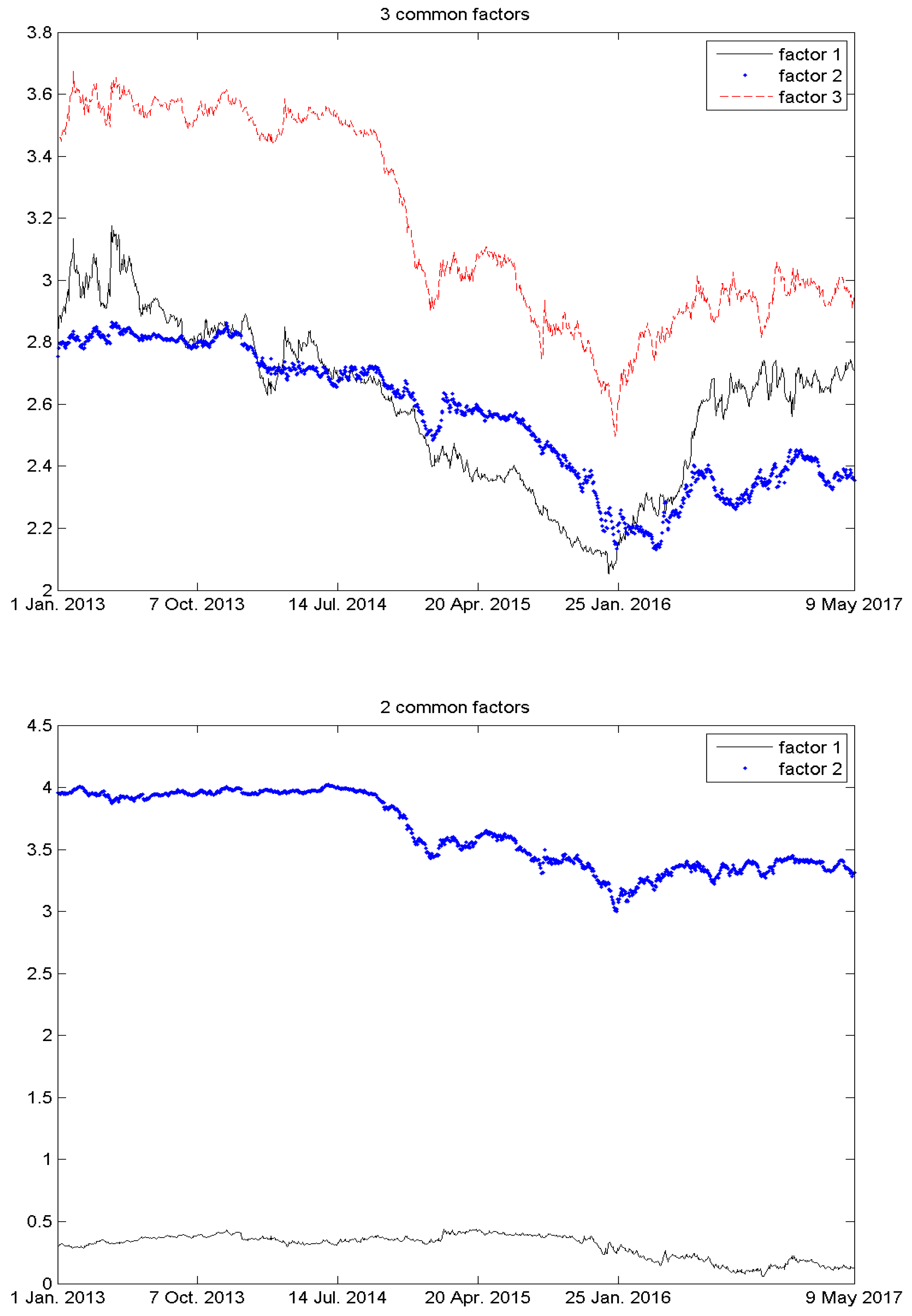
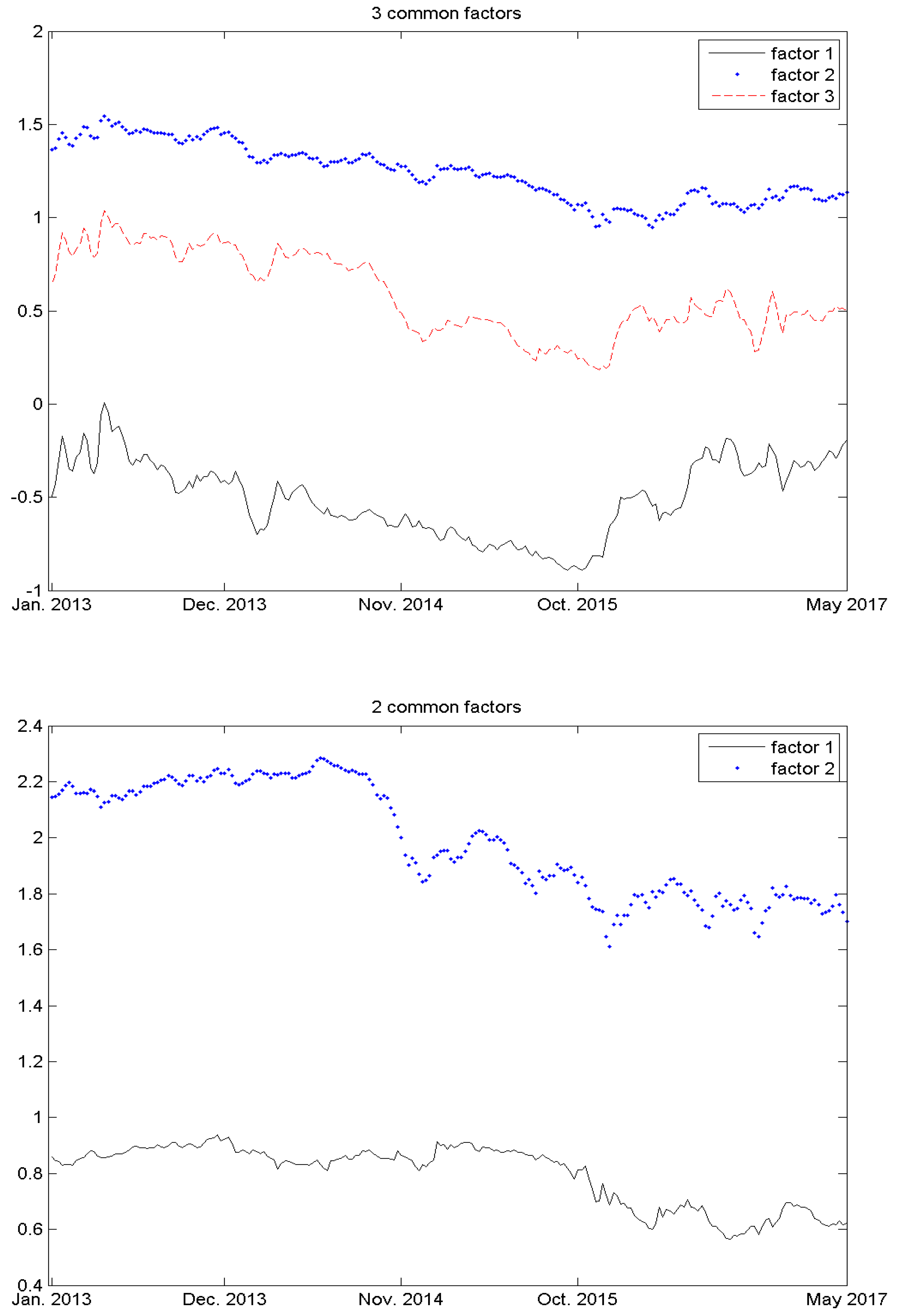
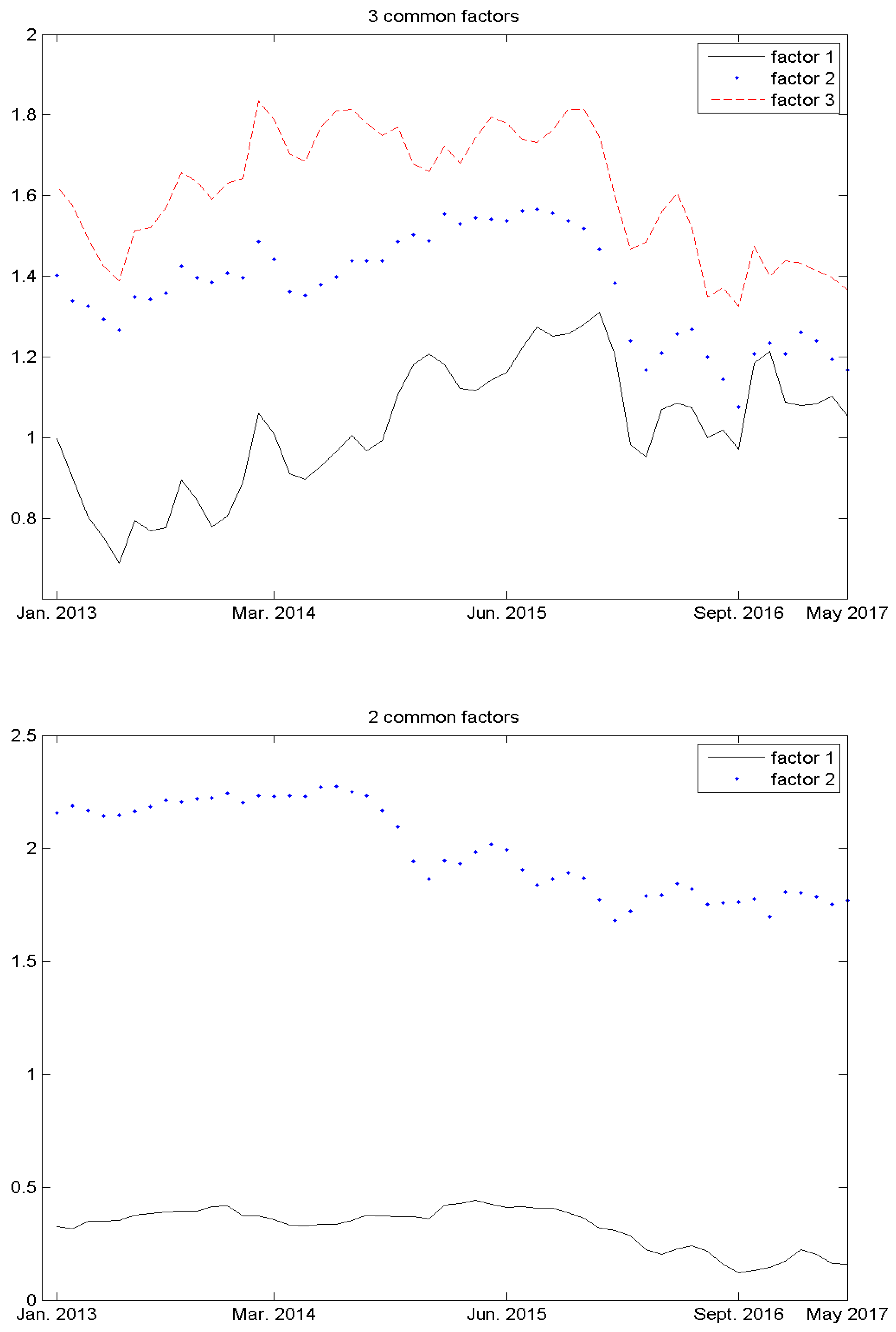
Figure 1, Figure 2 and Figure 3 shed further light on the dynamics of the common trends driving $Y_t$ and ${\tilde{Y}}_t$ at different frequencies. The results show overwhelming evidence of the differences between the permanent components driving the system of fuel prices when EUA prices are included and the permanent components when fuel prices are considered alone. These findings confirm the relevance of the EUA forward market in determining the dynamics of fuel forward prices. In particular, these figures show the existence of a very significant additional factor that influences the formation of fuel prices. The dynamics of these common factors are similar across data frequencies and provide further robustness to the results.

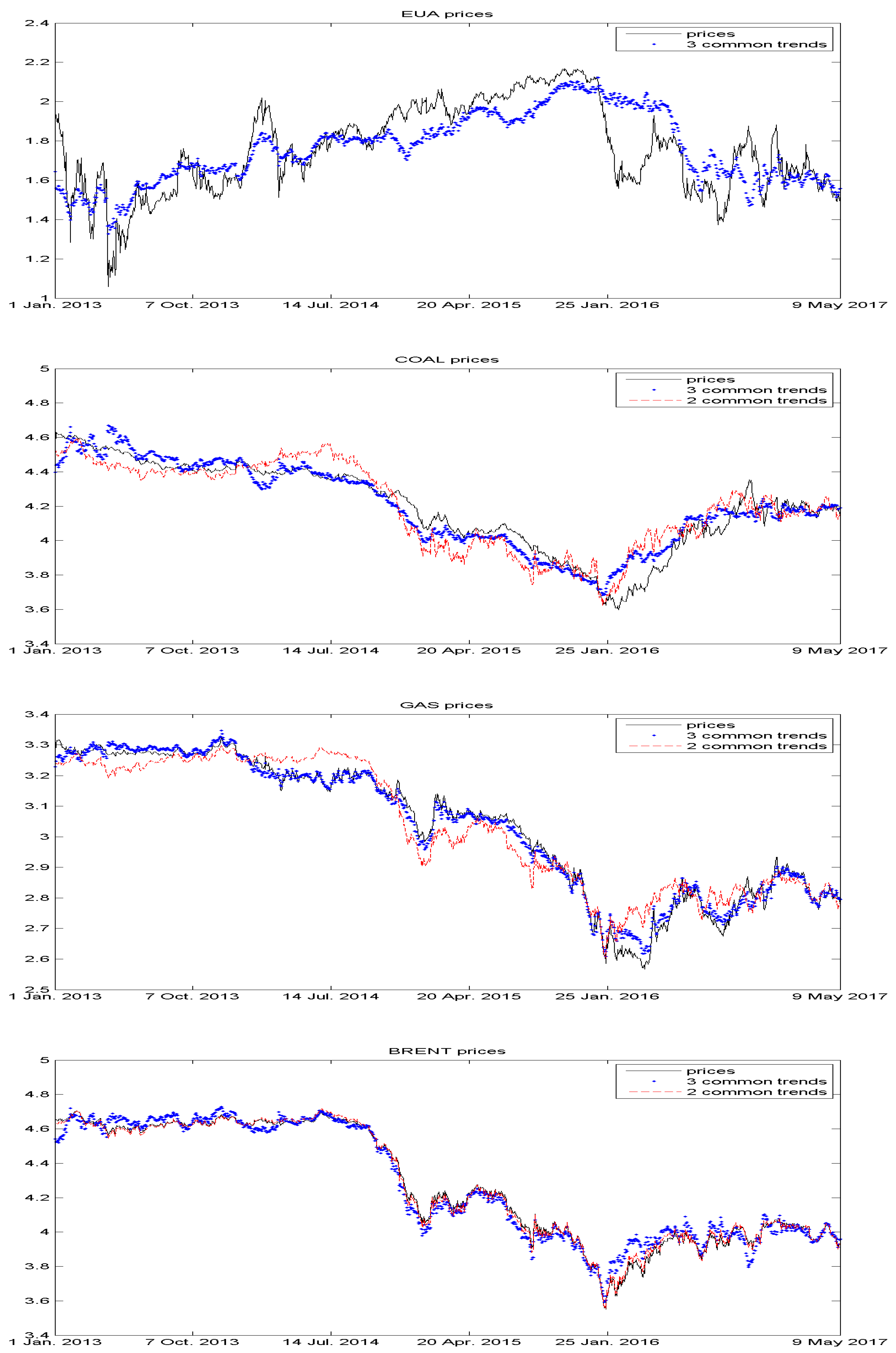
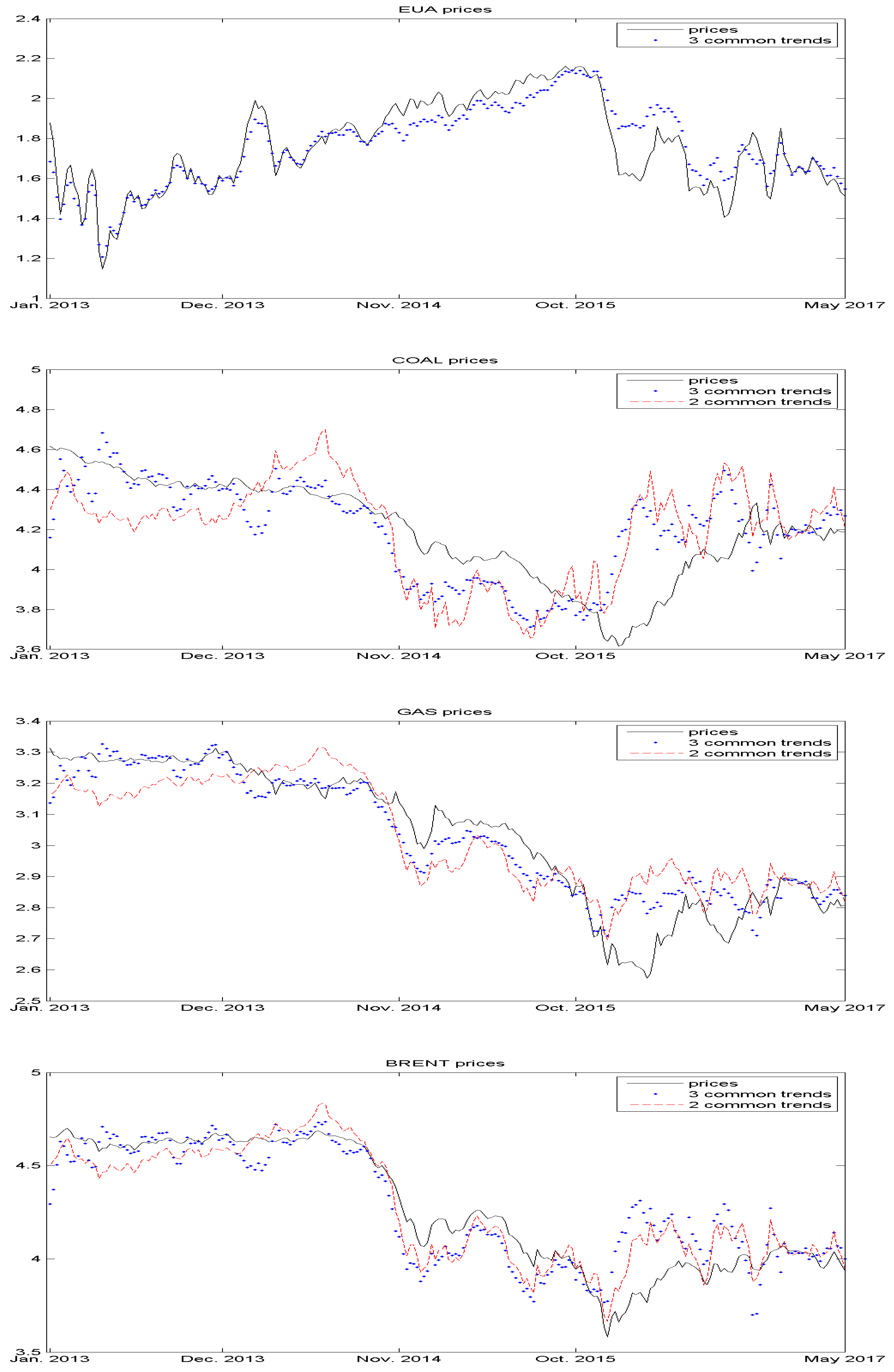
To complete the section, we have also plotted the estimates of the permanent component of the decomposition of the time series of prices. Figure 4, Figure 5 and Figure 6 contain these decompositions for each time series separately and also across different data frequencies. The top panel represents the dynamics of EUA prices along with the estimated permanent component captured by $A_1{f}_t$. The results show how the permanent component is able to reflect the trend of EUA prices. There is a period, however, at the end of January 2016 in which the permanent component fails to capture a dramatic fall in EUA prices. According to some traders, this drop in the price of carbon emission allowances could be explained by a high level of speculation in the market during that period, but also by an unexpected increase in the amount of emission permits released into the market. In our model, this is captured by the transitory component, suggesting, according to the Gonzalo–Granger decomposition, that it has no effect on the future evolution of EUA prices.

The remaining three panels display the dynamics of coal, gas and Brent oil along with the corresponding estimates of the permanent components. In these cases, the charts also contain the permanent component ${\tilde{A}}_1{\tilde{f}}_t$, with ${\tilde{A}}_1$ and ${\tilde{f}}_t$ obtained from the permanent-transitory decomposition of the time series ${\tilde{Y}}_t$. The findings of this study reveal a better performance of the model with three common factors in describing the dynamics of coal and gas. To add more rigour to the analysis, we compute the mean squared error between the actual time series, e.g., coal, and the corresponding permanent component $A_1{f}_t$ or ${\tilde{A}}_1{\tilde{f}}_t$, respectively. For the analysis of coal prices with daily data, we obtain a mean squared error of $0.0723$ for the model with three factors and $0.1024$ for the model with two factors. Similarly, for the analysis of gas prices with daily data, we obtain a mean squared error of $0.0216$ for the model with three factors and $0.0618$ for the model with two factors. The results are, however, reversed for the analysis of Brent oil. In this case, we obtain a mean squared error of $0.0495$ for the model with three factors and $0.0145$ for the model with two factors. Interestingly, the common factors obtained from only considering fuel prices provide a better fit of the time series of oil prices.

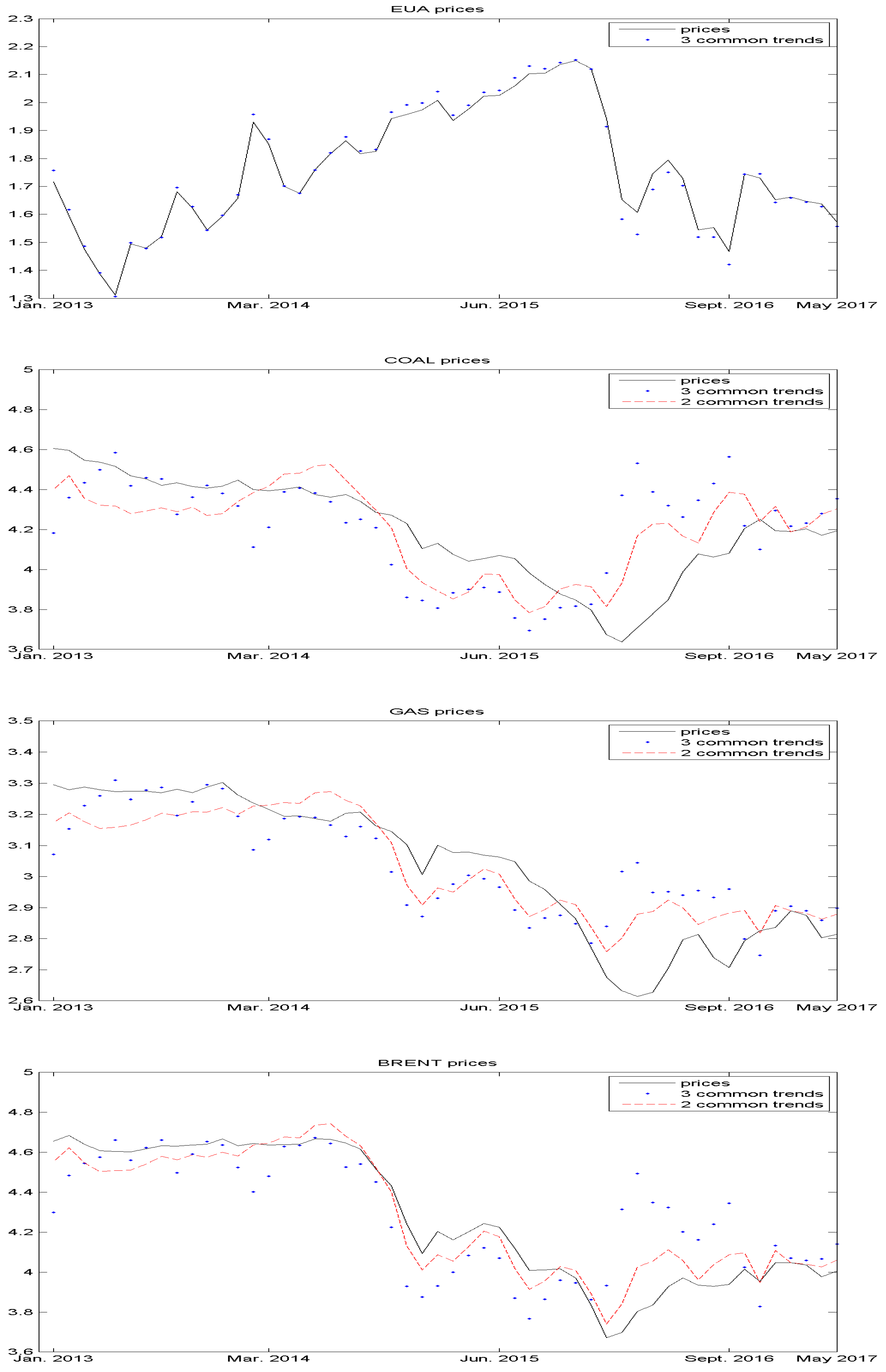
The analysis of weekly data in Figure 5 presents similar findings. In this case, it is perhaps easier to observe from the graphs the better fit of the permanent component for coal and gas obtained from the model with three factors than with two factors. Nevertheless, for completeness, we report the mean squared error between the actual commodity prices and the permanent components for weekly and monthly frequencies. Thus, for the analysis of coal prices with weekly data, we obtain a mean squared error of $0.2021$ for the model with three factors and $0.2433$ for the model with two factors. Similarly, for gas prices with weekly data, we obtain a mean squared error of $0.0771$ for the model with three factors and $0.1134$ for the model with two factors. For Brent oil and weekly data, we obtain a mean squared error of $0.1586$ for the model with three factors and $0.1160$ for the model with two factors.

The analysis of monthly data is reported in Figure 6. In this case the results are reversed, and the common factors obtained from only considering fuel prices provide a better fit of coal, gas and Brent oil than the model that also benefits from information on EUA prices. More specifically, for the analysis of coal prices with monthly data, we obtain a mean squared error of $0.2671$ for the model with three factors and $0.1803$ for the model with two factors. Similarly, for gas prices, we obtain a mean squared error of $0.1400$ for the model with three factors and $0.1038$ for the model with two factors. Finally, the analysis of Brent oil reports a mean squared error of $0.2245$ for the model with three factors and $0.0873$ for the model with two factors.

5. Conclusions

This paper studies the relationship between the prices of EU carbon emission allowances and fuel prices, in particular, coal, gas and Brent oil during Phase 3 of the EU ETS. To do this, we have explored long-run and short-run relationships using a dynamic VAR specification for the time series of log-prices for spot and forward markets. The results provide overwhelming evidence of a long-run equilibrium relationship between forward markets of the three commodities and EUA prices; however, we find no statistical evidence of cointegration between spot prices. These results suggest that EUA and fuel spot prices move independently and cannot be explained by a set of common factors. In contrast, the analysis of the corresponding forward prices reveals a cointegration relationship between these prices. These results show that the forward prices of EUA and fuel are endogenously determined with permanent components driven by three common trends.

The presence of a VECM representation also allows us to obtain a decomposition of the price series in terms of a permanent and a transitory component. The permanent component is a combination of prices of EUA and fuels. This combination uncovers the relevance of the market for EUA in determining the series of fuel prices. Statistically, the inclusion of EUA prices in the vector of fuel prices improves the fit of the time series of coal and gas. Our results are robust to different specifications of the VAR and VECM equations and, more importantly, to the frequency of the data in Phase 3.

The analysis of the robustness of our results to data from Phases 1 and 2 of the EU ETS remains to be studied. The answer to this question is left for future research, as there are many salient features of the market for emission allowances that have changed between phases. We also leave for further research the implementation of VECM procedures that take into account the presence of conditional heteroscedasticity in the dynamics of returns at different frequencies.