Exergy As a Measure of Sustainable Retrofitting of Buildings

Abstract

This study presents a novel optimization methodology for choosing optimal building retrofitting strategies based on the concept of exergy analysis. The study demonstrates that the building exergy analysis may open new opportunities in the design of an optimal retrofit solution despite being a theoretical approach based on the high performance of a Carnot reverse cycle. This exergy-based solution is different from the one selected through traditional efficient retrofits where minimizing energy consumption is the primary selection criteria. The new solution connects the building with the reference environment, which acts as “an unlimited sink or unlimited sources of energy”, and it adapts the building to maximize the intake of energy resources from the reference environment. The building hosting the School of Architecture at the University of Navarra has been chosen as the case study building. The unique architectural appearance and bespoke architectural characteristics of the building limit the choices of retrofitting solutions; therefore, retrofitting solutions on the façade, roof, roof skylight and windows are considered in multi-objective optimization using the jEPlus package. It is remarkable that different retrofitting solutions have been obtained for energy-driven and exergy-driven optimization, respectively. Considering the local contexts and all possible reference environments for the building, three “unlimited sinks or unlimited sources of energy” are selected for the case study building to explore exergy-driven optimization: the external air, the ground in the surrounding area and the nearby river. The evidence shows that no matter which reference environment is chosen, an identical envelope retrofitting solution has been obtained.

1. Introduction and Motivation of the Work

Construction is at the centre of social and economic activity and represents one of the biggest economic sectors [1]. When discussing the energy used in buildings, it is important to consider that it represents almost 40% of the total energy consumption in the world [2], and therefore, greater efficiency can make a key contribution in the climate change mitigation scenario, as was highlighted at the 21st Session of the Conference of the Parties of the United Nations (UN) Framework Convention on Climate Change (COP21) [3]. In Europe, many efforts have been made in the political [4] and scientific field to produce a more sustainable building energy portfolio. The Energy Performance of Buildings Directive (EPBD) was recast in 2010 to make the goals more ambitious and to reinforce the implementation of energy efficiency measures [5]. This implementation depends, however, on the commitment of stakeholders, industry and civil society. Since then, a wide array of measures has been adopted across individual Member States to promote a better energy performance of buildings actively. As strategies evolve and become more complex, stakeholders need more concrete and precise facts and tools to be able to make comparisons and to implement the monitoring systems that permit the quantification of advances and progress in the various Energy Conservation Measures (ECM).

When considering improving the energy performance of buildings, one option is to optimize the scheduling of building energy consumption. Nowadays, there is a growing interest in improving energy efficiency by choosing the best building energy consumption strategy or operational option. As a result, reliable building energy models including behavioural models [6] are often needed to support the demand response programs. From that perspective, the building energy model plays a very important role because of its unique features such as model predictive control, which uses models to analyse the opportunities of the energy market (electricity, fuels, etc.). These models could be statistical (mathematical models based on data for the estimation of total energy demand) or physical (mathematical equations that represent all the physical properties of a building). Some examples of the former can be observed in [7,8,9] and of the latter in [10,11,12].

On the other hand, this manuscript considers an approach based on retrofitting existing buildings as a way of improving building energy performance. It is a complex task that requires a thorough evaluation because buildings and their environments are complex systems. According to research by Asadi [13], when discussing retrofitting, two approaches can be considered: conventional and multi-objective optimization. In the conventional method, the alternative retrofitting solutions are a combination of known variables with different results; each variable has a different weight, and the combination of weights produces the best solution. Examples of this evaluation methodology can be seen in [14,15,16,17]. In the multi-objective optimization method, a model, which may be, as mentioned before, physical or statistical [18], in combination with an optimization program, automatically produces a set of solutions. This approach is supported by several studies [19,20,21,22,23,24]. In this paper, we have selected a multi-objective optimization method based on a physical model. The physical model can be developed by different software programs such as EnergyPlus [25] or TRNSYS [26]. The capacity of these models to evaluate the energy performance of buildings is well documented [27].

In this study, our goal is to provide an exergetic approach to the problem of the energy performance of buildings. Exergy adds a new concept: the quality of energy. Exergy can be defined as the maximum theoretical work that can be extracted from a combined system consisting of the system under study and the environment as the system passes from a given state to equilibrium with the environment [28].

Nowadays, we are focused on reducing energy consumption, but strictly speaking, energy cannot be consumed, but transformed [28]. In contrast, exergy can be destroyed because is exposed to irreversible processes. This destruction provides us with clues as to how efficiency in buildings can be improved. There is energy everywhere; however, energy does not always have the necessary quality to serve our purposes, and it is necessary to reflect on how we can use this low-quality energy in a more efficient way. As has been studied intensely in [29,30], heating and cooling in buildings can be carried out with low grade energy, meaning with energy of low exergy. Why do we use a fluid at a high temperature from $40$–$80{}^{\circ }$C when the air in a building could be around 23 ${}^{\circ }$C? For this reason, the concept of exergy should start to play a more critical role when discussing the performance of buildings.

The concept of exergy brings up another important aspect: the environment. Building design should take into account the surrounding environment because the environment can provide opportunities for saving energy, as has been studied by Meggers and Leibundgut [31]. Exploitation of the energy that can be found in our immediate environment by the natural ventilation and thermal mass of building envelopes should be considered, and exergy is the right tool to do so. As an example, at night, outdoor air, with a lower temperature, could flow in to reduce the internal heat and to contribute to cooling the internal surfaces for the next day. In these circumstances, the environment works as a cold sink that helps us to take away heat from the building (the hot source). Therefore, the exergy concept provides us information on the amount of work that can be saved in that situation, as will be explained later [32].

Exergy puts the environment in contact with the building through the envelope by consuming the energy demand. The energy demand of a building can be defined as the amount of energy required to keep the indoor temperature within the comfort ranges required by its users [29]. In winter, 100% of the energy demand is consumed by the envelope. The idea of this work is to consider different environments in order to optimize the building envelope components.

Following the above reflection, the buildings of the future should maximize their performance taking into consideration the environment in the same way that trees do. For example, the tree shape is the result of competition for resources: competition between branches for light and space and competition between roots for nutrients and water. On the other hand, the trees are affected by global properties of the environment such as day length, controlling the initiation of flowering, and daily minimum and maximum temperatures, modulating the growth rate. Similarly, the tree is affected by local properties of the environment, such as the presence of obstacles, which control the spread of grass and direct the growth of the roots of tree. The result of this interaction is adaptation to the environment and efficiency in the use of the available resources [33,34].

This idea of the adaptation of buildings to the environment is the concept that we want to pose in this paper. Exergy is a concept that measures energy quality, but in reference to a selected environment, and for that reason, it offers us the opportunity to connect the building with the environment in order to maximize the resources in a similar way to a tree. Accordingly, in this work, the optimization of building exergy performance is based on the idea of connecting the building with the different environments available. On the one hand, when referring to energy demand, one of the most sensitive components is the building envelope, and it is of great interest to check how this exergy optimization concept can affect it. On the other hand, it is one of the components that is easiest to refurbish in an existing building, as explained by Sozer [35]. Many works have been carried out regarding the exergetic optimization of other components from generation to distribution, as shown in Figure 1, of the energy supply chain. Among these, [36,37,38] can be highlighted, but our proposal seeks to focus the optimization process on the more architectonic part of the building: the envelope, on which there are fewer studies. The methodology of exergy demand calculation is based on the IEA-EBCAnnex 49 recommendation [29] by Schmidt [39]. The manuscript implements a novel approach to handle the problem of temperature fluctuation in order to classify the different types of exergy adequately. The study was performed in a dynamic building energy simulation tool EnergyPlus. This exergy classification allows distinguishing between the exergy that is coming from environmental sources and the exergy of fuels. The optimization process will maximize the former and minimize the latter.

The paper is organized as follows. Section 2 examines how a dynamic analysis of the energy demand of a thermal model can be transformed into an exergy balance, which is the simplifications that are considered in the process. Section 3 explains how this paper solves the problem of computing different types of exergy when the environment is taken into account, the characteristics of the different environments that have been used and how the problem of the fluctuating temperatures has been addressed. Section 4 explains in detail all of these stages. There is a description of the model and the main components of the building that will play a role in the optimization process. It also shows how the energy calculation is performed, bearing in mind the operational schedules of the building and the connection between the energy model and the optimization program. In addition, an explanation of the objective function and the algorithm that are going to be used are exposed. In Section 5, graphs depicting the optimization results are explained; finally, in Section 6, the conclusions of this exergetic analysis are shown.

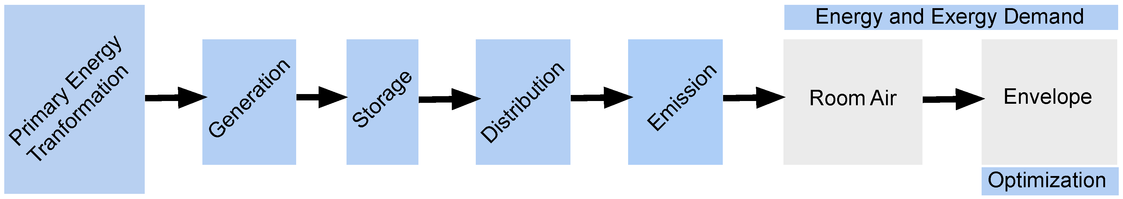
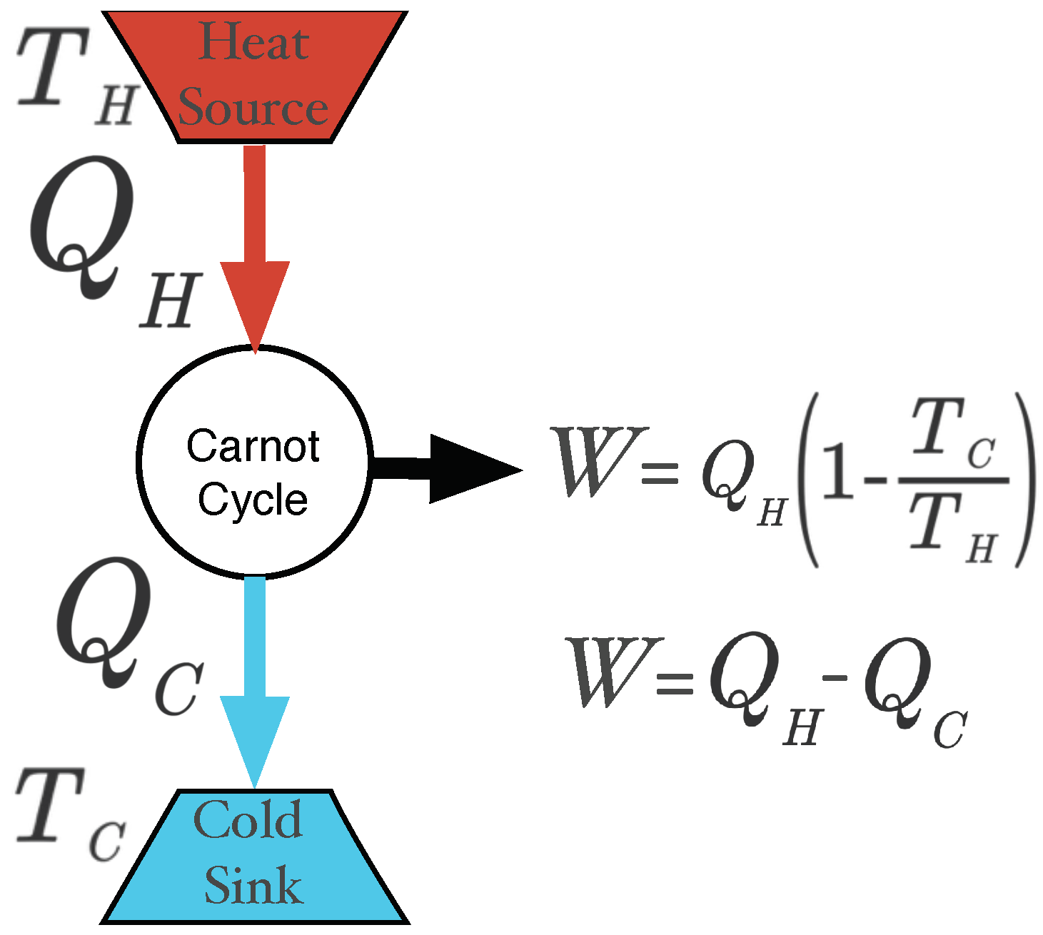
2. Energy and Exergy Demand

A very important step to determine the energy balance is the calculation of the energy demand. As has been explained in Annex 49 [29], the exergy demand cannot be calculated using energy balance equations. Therefore, the exergy demand must be calculated from the results of the energy balance equation. For this purpose, a dynamic simulation program such as EnergyPlus was selected. This program provides the building energy demand at hourly time steps. The energy demand represents the theoretical minimum amount of energy required by the thermal zones in order to maintain the zone temperature within range.

This minimum demand is only related to the component building envelope, and it is not related to the subsystems that provide heating (HTG) or cooling (CLG), as can be seen in Figure 1. Accordingly, demand is the objective function that we use in order to optimize the different components of the envelope.

A simplified exergy demand calculation, as is described in Annex 49 [29] and developed by Schmidt [39], has been used. The main simplification of this approach is that the energy demand has the quality of heat (or cold), and it is supplied at the temperature of the thermal zone. The exergy of heat is based on a reversible Carnot cycle [40] working between two temperatures, as is indicated in Figure 2. This way, the exergy demand can be calculated using Equation (3) or (4) taken from the first and the second principle of thermodynamics (see Equations (1) and (2)).

$$Q_H=Q_C+Ex$$

(1)

$${\displaystyle \frac{Q_H}{T_H}}={\displaystyle \frac{Q_C}{T_C}}$$

(2)

$$Ex=Q_H\left(1-{\displaystyle \frac{T_C}{T_H}}\right)$$

(3)

$$Ex=Q_C\left({\displaystyle \frac{T_H}{T_C}}-1\right)$$

(4)

where:

• $Q_H$ = Energy flow from the heat source (kWh).
• $Q_C$ = Energy flow to the cold sink (kWh).
• W = Exergy (kWh).
• $T_H$ = Temperature of the heat source (${}^{\circ }$K).
• $T_C$ = Temperature of the cold sink (${}^{\circ }$K).

Characteristics of the simplified exergy demand calculation:

• It only takes into account the thermal component of the energy demand; the chemical or pressure components are not included. This is reasonable as long as no (de)humidification is present.
• The calculation is based on the idea that the energy demand will be supplied as convective heat. In general, energy demand is supplied in part as convective heat and in part as radiative heat. In our study, this simplification is acceptable because there is no radiative system.
• The calculation method implies that the energy is supplied as heat at a fixed temperature. It does not take into account the energy needed for the climatization of the ventilation air.

This method considers the building as a closed system, and this means that for the evaluation of the envelope performance, the results are acceptable as noted in Annex 49 [29]. On the other hand, when trying to optimize heating and ventilation systems, a more detailed calculation is needed. Figure 1 summarizes the target of the optimization.

3. Reference Environment

The reference environment can be described as “that portion of the surroundings of a system, of which the intensive properties of each phase are uniform and do not change significantly as a result of the process under consideration” [41]. In other words, the environment can act as an unlimited sink or unlimited source [42]. For this reason, the referent environment cannot be chosen arbitrarily, because of its strong influence on the exergy balance [43].

In our case, we have selected three different reference environments to compare which one can offer the best envelope optimization scenario for a building. Each of them complies with the requirements exposed in Annex 49 [29]:

• unlimited (either acting as a sink or a source),
• unchanged by the processes that are regarded,
• always available.

If we consider that a building can interact with the environment and that perhaps in the future, heating (HTG) and cooling (CLG) systems can perform in a way that could change the sink and the source in order to connect with the place where more energy will be available, this theoretical reflection could be useful. The main characteristics of each of the environments are described in the following paragraphs.

(a)

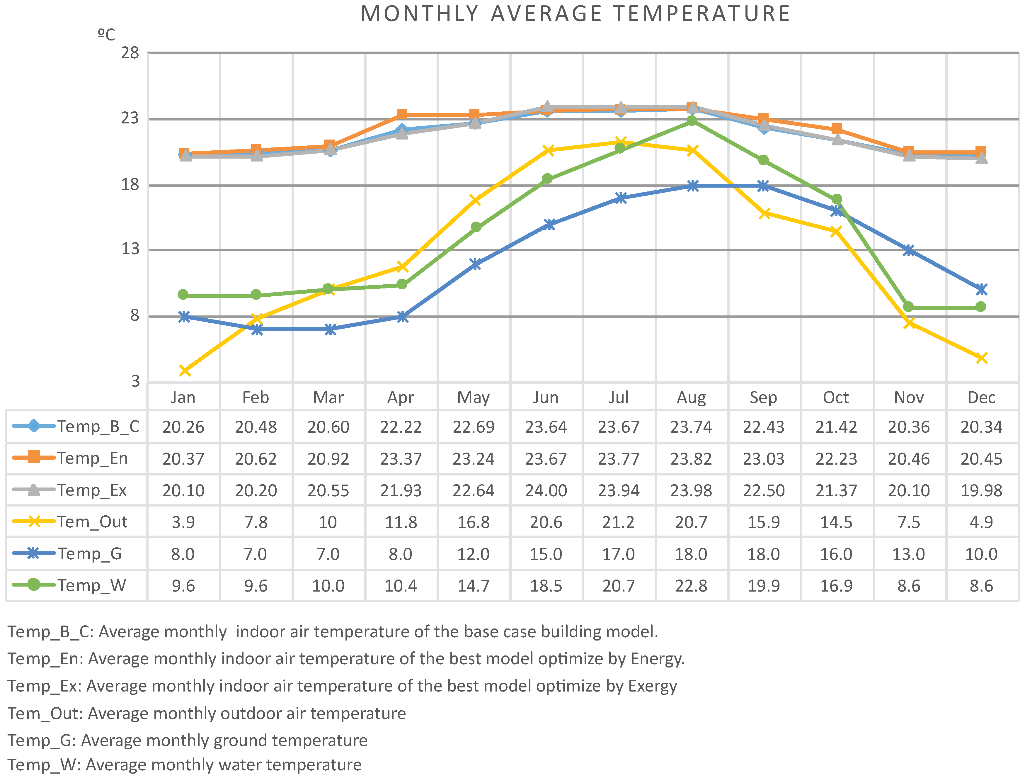
The ambient air surrounding the building: The air around could be the sink and the source, with a certain capacity so that no changes in its temperature, pressure or chemical composition can affect the system. This sink (or source) is free and easy to access. The information has been taken from a meteorological station located at the School of Architecture. For the exergy balance, the temperature has been taken at an hourly time step and combined with the indoor air temperature of each model. It is the only case where hourly temperature has been used; in the other cases (water and ground), the temperature used is the monthly average. It is represented in Figure 3 on a monthly basis in order to compare it with the other temperatures.

(b)

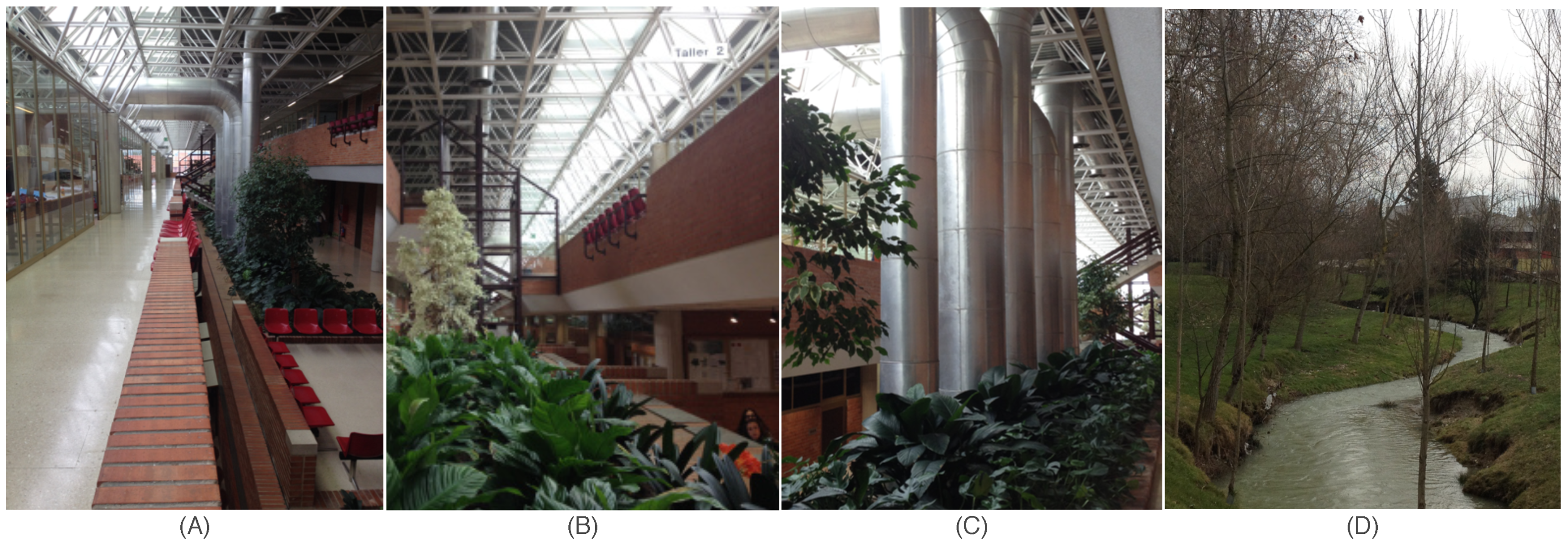
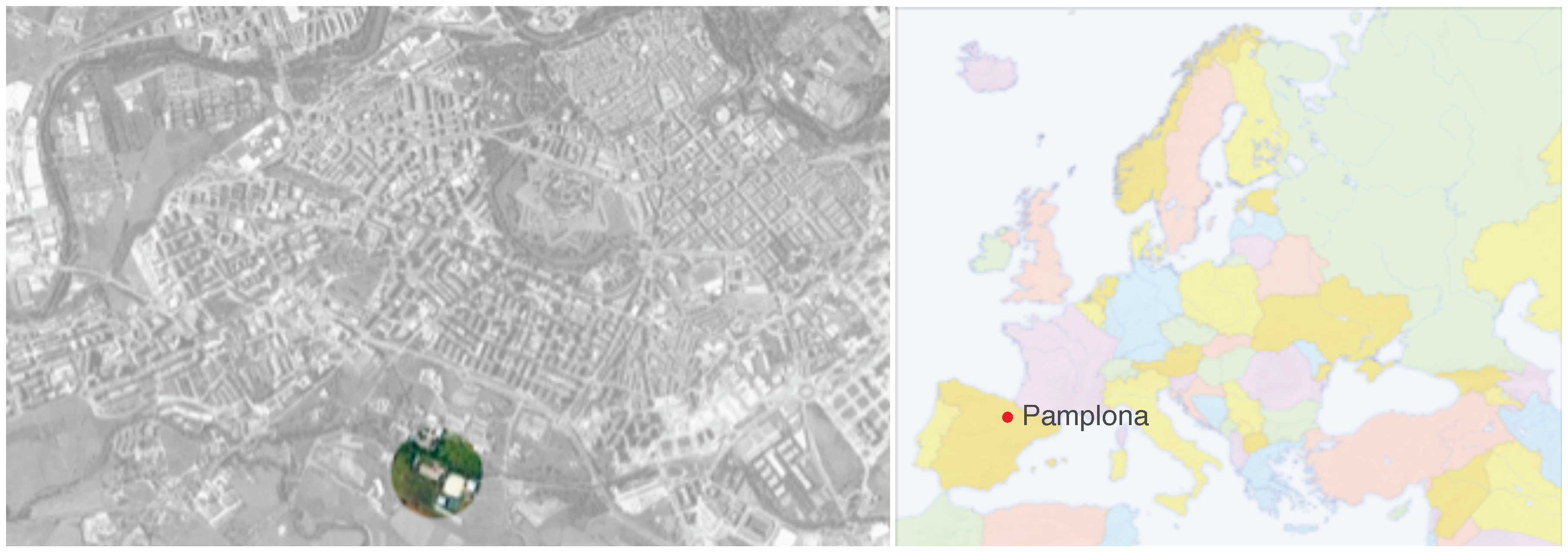
The ground under the building or in a nearby area: As the building selected is in a natural location without other buildings around (see Figure 4), it is possible to have easy access to the surrounding ground. Additionally, the ground under the building is available and accessible because the foundations are not covered. Utilizing the software climate consultant [44], the temperature data at a depth of 3 m have been taken at a monthly time step based on the information from the in situ weather station. The data are presented in Figure 3.

(c)

The nearby Sadar River, which can be seen in Figure 5D, is another possibility for the environment context of this building. The river crosses the building parcel under a tunnel. This makes it possible to build a small dam and to install a water-to-water heat exchanger. The Sadar River is a tributary of the Arga River, and the data of the temperature have been taken from the information provided by the local government of Navarra [45] on a monthly basis, as Figure 3 shows.

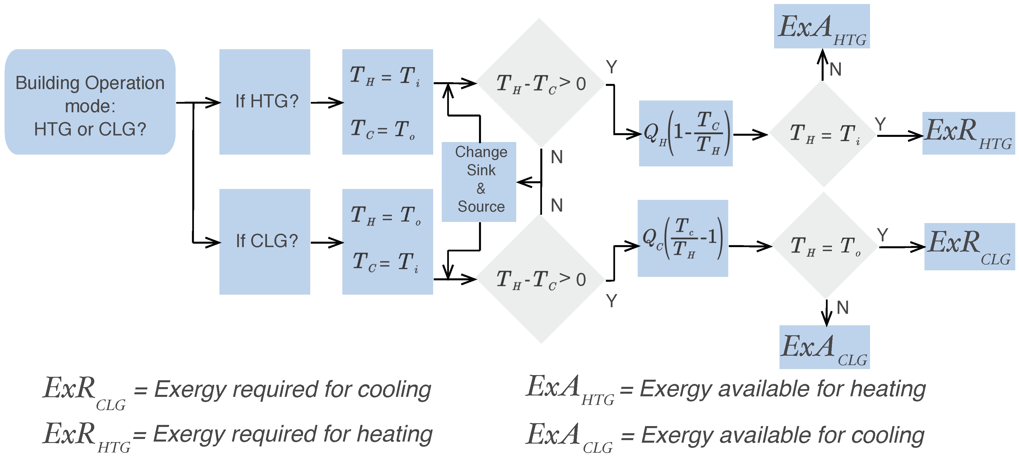
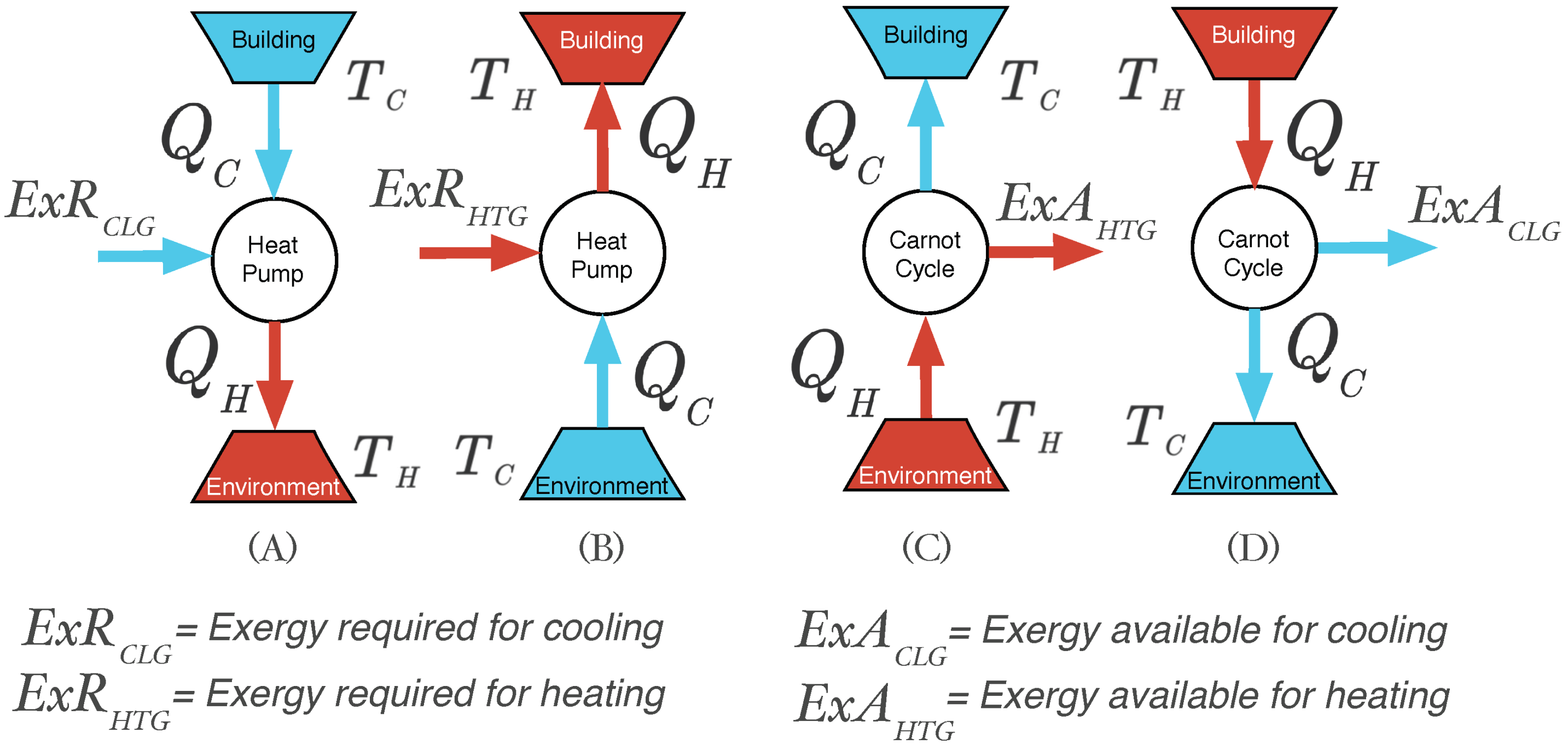
The Concept of Exergy Available and Exergy Required

From an energy point of view, heating demand means energy is an input, and cooling demand means energy is an output. As explained with regard to exergy demand, it is necessary to consider the temperature of the reference environment. Figure 6 demonstrates the different situations that can take place in relation to the reference environment. In Figure 6A,B, the system is working as a heat pump (HP), and therefore, exergy is required (ExR) for HTG and CLG so that the building can satisfy its energy demand. In Figure 6C,D, the cycle is working in a reversible way, and there is exergy available (ExA) for HTG and CLG. In this situation, the Carnot cycle informs us that we can use the environment in order to meet the building energy demand. The fluctuation in the temperature of the environment produces exergy variations, which affect Equations (3) and (4), producing negative results, but exergy has to be positive, because negative work does not exist. Therefore, to avoid this problem, some authors write Equations (3) and (4) between absolute brackets [46]:

$$Ex=Q_H\left|1-{\displaystyle \frac{T_C}{T_H}}\right|$$

(5)

$$Ex=Q_C\left|{\displaystyle \frac{T_H}{T_C}}-1\right|$$

(6)

ECBCSAnnex 49 [29] notes that this procedure has to be used with care, because by using Formulas (5) and (6), the information related to the direction of the exergy is lost. This problem was stated in detail by Pons [47], and because of that, the recommendation is to fix the reference state. A study taking into account this approach was carried out by Bonetti et al. [24], where the authors focused on the potential for thermal storage in the envelope, and they used a reference environment at a fixed temperature of $26{}^{\circ }$C. Our approach is different and is explained in detail in the next paragraph.

As stated, EnergyPlus was the tool selected for the evaluation of the HTG and CLG demand in the different energy models proposed in this paper. EnergyPlus can provide many outputs for a dynamic energy analysis, but exergy is not among them. By using the EnergyPlus runtime language (Erl), we have developed specific outputs that can compute the exergy in the way shown in Figure 6, where the distinction of exergy required (ExR) and exergy available (ExA) is stated. This way, for each environment in each time step, we can collect the four different values of exergy. This process can be repeated for each environment, and twelve exergy values will be available. These values are used to compute the objective function in the optimization process carried out afterwards.

In Figure 7, there is a graphic description of how the script has been made. The idea is to check previously the value of each temperature before starting the computation of the formulas, so that in this way, we can classify the sink and the source in order to avoid negative values of the exergy. From a practical point of view, this script allows the performance of an exergy analysis despite fluctuating temperature in the reference environment. This procedure avoids the negative exergy results that according to Pons [47] could be computed as irreversibilities.

4. Design of the Experiment

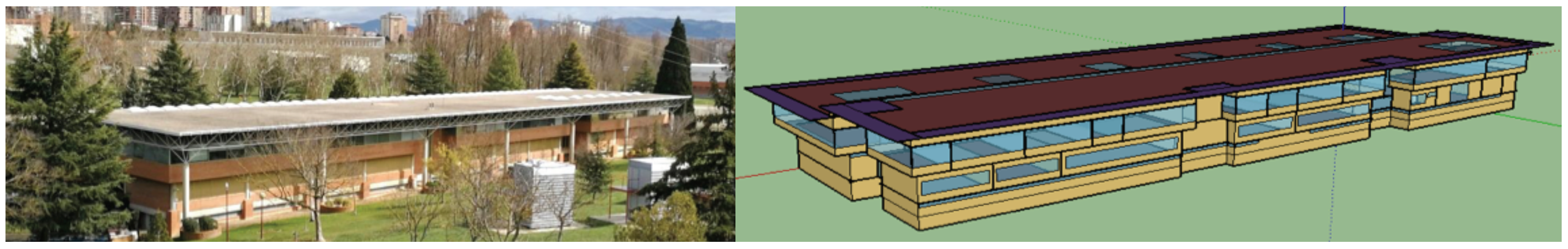
4.1. The Building and the Retrofitting Measures

The School of Architecture building is located on the campus of the University of Navarra in Pamplona (Figure 8) and has been selected for this experiment. The construction of the building was started in 1975 by the architects Carlos Sobrini, Rafael Echaide and Eugenio Aguinaga, and it was inaugurated in 1978. The building can be situated in the modernism movement, following the design philosophy of architects like Frank Lloyd Wright and Mies van der Rohe. It is characterized by simple materials, clean lines and ample light. The structure aesthetic is defined by brick, cast concrete, glass and steel. The building centres on a light-filled atrium, where the mixture of a ventilation system and different kinds of plants and trees creates a particular atmosphere, as can be seen in Figure 5.

The skylights in the roof are responsible for the light in this area and are, as will be explained afterwards, a key element of the process (see Figure 5A–C).

A simplified model of the building has been made, in which it has been assumed that the façades are made of two walls of perforated bricks separated by a non-ventilated air cavity of 10 cm, while the windows are composed of simple glasses with a value of 5.7 W/m${}^2$K and an SHGC of $0.83$. The floor has been assumed as a reinforced concrete slab of 30 cm thick, with $2.5$-cm gripping mortar and $2.2$-cm terrazzo. The roof is made of zinc-plated galvanized steel sheeting, 2 cm of XPSat 0.038 W/m${}^2$K, a layer of EPDM, a geotextile and 5 cm of gravel, with skylights with a transmittance of equal properties of the window glass. The partitions between are either of preformed brick or monolithic glass.

The building is open from Monday–Friday from 08:00–20:00 and on Saturday from 08:00–14:00 (this is the daily schedule for July and August); on Sunday, it is closed. As can be seen in Figure 5B,C, the HTG and the CLG come to the building as air through large ducts. The heat is produced by a gas boiler and cooled by an electric chiller. Different air handling units (AHU) distribute the air through ducts in the main areas of the building. There are three main seasons for the air conditioning; the first is called $1\_Term$ and covers the months of: January, February, March and April. The second is called $2\_Term$ and covers the months of: May, June, July, August and September. The $3\_Term$ includes the months of October, November and December. The setpoints complied with the Spanish legislation on health and safety measures [48]; $21{}^{\circ }$C for heating, $25{}^{\circ }$C for cooling, with a maximum zone air temperature of $27{}^{\circ }$C in the cooling season and $17{}^{\circ }$C in the heating season. All of the models used comply with these criteria. The system cannot provide cooling in the $1\_Term$ and $2\_Term$, nor heating in the $3\_Term$.

The model has 45 different thermal zones. In order to simplify the calculation, however, the exergy has been computed as the average temperature of each zone. A script in Erl has been developed to obtain that temperature as an output of EnergyPlus. This average temperature is that which is used as the indoor temperature in the exergy Formulas (3) and (4). The monthly average indoor air temperature of the three cases under study has been plotted in Figure 3. The internal loads of the building could be summarized as 1 W/m${}^2$. The time step considered for energy balances is one hour. As the HVAC systems are not going to be considered in the optimization process as was stated before, the model is configured for ideal load systems.

In order to find the best envelope that adapts to the different environments, it is necessary to choose the most suitable components that can be modified. The aesthetic considerations of the building and its architectural personality make it difficult to implement retrofitting measures easily. Bearing in mind the different dimensions of the components of the envelope (see

Table 1. Different dimensions of the envelope components.

	Total	North	East	South	West
Wall Area (m${}^2$)	3125.45	1121.77	373.11	1189.01	441.56
Window Area (m${}^2$)	983.65	400.37	87.07	409.11	87.1
Façade total Area (m${}^2$)	4143.53	1539.1	447.49	1640.91	516.02
Skylight Area (m${}^2$)	664.65	-	-	-	-
Roof Total Area (m${}^2$)	4290.70	-	-	-	-

), we have chosen three areas of intervention. The first is the possibility of improving the insulation in the roof, which can be carried out without affecting any aesthetic characteristic of the building. The second one is the modification of the glass panels of the windows and skylights; these represent 983.65 m${}^2$ and 664.65 m${}^2$ respectively (Table 1), which amounts to $19.5$% of the total area of the envelope (8433.7 m${}^2$). The external frame of the windows has to be maintained in order not to modify the aesthetic of the façade. Different options for each orientation have been selected. On the other hand, the skylight panel can be changed with the criterion of not modifying the building aesthetics.

The third area for retrofitting measures is the walls. For this component, the more efficient option is to fill the air cavity with a unique insulation component. As can be seen in Figure 4 and Figure 5, the red brick element is a very important component of the design of the building.

Table 2. Different parameters for the envelope configuration.

Construction	Orientation	Element	Parameter	B_C	V_1	V_2	V_3	V_4
Façade	North	Insulation	Thickness (cm)	0	10	-	-	-
	South	Insulation	Thickness (cm)	0	10	-	-	-
	East	Insulation	Thickness (cm)	0	10	-	-	-
	West	Insulation	Thickness (cm)	0	10	-	-	-
Roof		Insulation	Thickness (cm)	2	5	10	-	-
Roof Skylight		Window glass	U(W/m${}^2$K)	5.7	3.3	2.5	1.5	1.2
			$SHGC$	0.83	0.75	0.3	0.3	0.29
Windows	North	Window glass	U(W/m${}^2$K)	5.7	3.3	2.5	1.4	1.1
			$SHGC$	0.83	0.75	0.59	0.59	0.58
	South	Window glass	U(W/m${}^2$K)	5.7	3.3	2.6	2.7	2.6
			$SHGC$	0.83	0.75	0.11	0.46	0.46
	East	Window glass	U(W/m${}^2$K)	5.7	3.3	2.6	2.7	2.6
			$SHGC$	0.83	0.75	0.3	0.3	0.29
	West	Window glass	U(W/m${}^2$K)	5.7	3.3	2.6	2.7	2.6
			$SHGC$	0.83	0.75	0.11	0.46	0.46

summarizes the different elements and the values for each parameter that has been considered in the process of optimization. The combination of all the possibilities totals $15·{10}^4$, and it is called the search space where the multi-objective optimization algorithm has to find the most suitable combination in accordance with the criteria that have been fixed previously. This will be explained in detail in the discussion regarding the objective function.

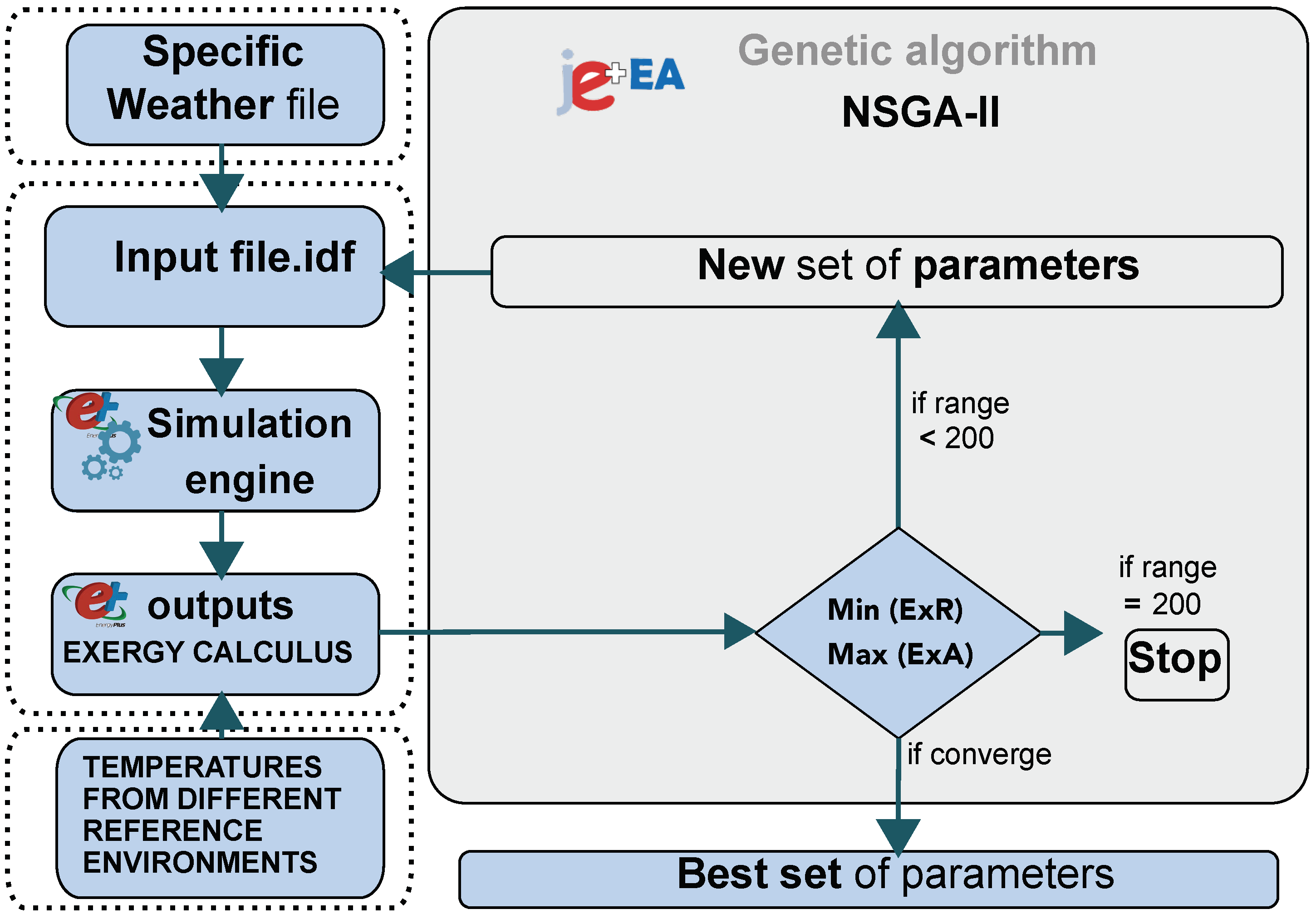
4.2. Simulation and Optimization Tools

The multi-objective optimization process selected in this paper is based on the search for an optimal solution among all the possible configurations described in the previous section. For the optimization engine, the package jEPlus was used [49]. This package combines the search performed by the genetic algorithm with the calculation performed by the EnergyPlus engine. As the energy outputs were previously prepared in EnergyPlus, the connection with the optimization package was very easy and is summarized in Figure 9.

The genetic algorithm is an evolutionary algorithm that operates on a finite set of simulations (population). In each iteration (generation), there is a competition between the different subjects (particular models) of the population, and the algorithm selects the ones that fit best with the objective. It then generates a new population for the next generation with the best subjects and new random ones. The population size used in this calibration procedure is 10, and the maximum value of generations is 200 [50].

The particular multi-objective evolutionary algorithm used is NSGA-II (Non-Dominated Sorting Genetic Algorithm II); its advantages compared to other algorithms are explained by Deb et al. [51]. NSGA-II uses a non-dominated sorting approach that achieves a better spread of solutions and convergence than other multi-objective evolutionary algorithms.

The objective function is the stimulus for the algorithm in order to find the optimal solution. The definition of a good objective function is a key element in the formulation of the problem. Because of that, each experiment requires a careful selection of the objective function. The authors have extensive experience on working with different objective functions in the same simulation environment [50,52,53].

Two experiments were carried out. In the first, the objective function was the minimum energy demand required for HTG ($E_1{\left(x\right)}_{min}$) and CLG ($E_2{\left(x\right)}_{min}$). This experiment has been performed previously by several authors [22,23]. The idea is to achieve an optimal configuration of the envelope in order to comply with the requirements of low energy consumption.

$$E_1{\left(x\right)}_{min}=\sum _{i=1}^n\left(HTG\left(t_i\right)\right)$$

(7)

$$E_2{\left(x\right)}_{min}=\sum _{i=1}^n\left(CLG\left(t_i\right)\right)$$

(8)

In the second experiment, the objective function is focused on exergy. In this case, the idea is to minimize the exergy required ($Ex{R}_{HTG}$, $Ex{R}_{CLG}$) and to maximize the exergy available (($Ex{A}_{HTG}$, $Ex{A}_{CLG}$); this experiment should be repeated three times in order to find the best envelope configuration for each of the environments that have been chosen: air ($a_1{\left(x\right)}_{min}$, $a_2{\left(x\right)}_{max}$), ground ($g_1{\left(x\right)}_{min}$, $g_2{\left(x\right)}_{max}$) and water ($w_1{\left(x\right)}_{min}$, $w_2{\left(x\right)}_{max}$). The scripts explained in Figure 7 and the special outputs developed in EnergyPlus will help to reconfigure the system easily in order to produce new results. In the next section, the results are analysed.

$$a_1{\left(x\right)}_{min}=\sum _{i=1}^n\left(Ex{R}_{HTG}\left(t_i\right)+Ex{R}_{CLG}\left(t_i\right)\right)$$

(9)

$$g_1{\left(x\right)}_{min}=\sum _{i=1}^n\left(Ex{R}_{HTG}\left(t_i\right)+Ex{R}_{CLG}\left(t_i\right)\right)$$

(10)

$$w_1{\left(x\right)}_{min}=\sum _{i=1}^n\left(Ex{R}_{HTG}\left(t_i\right)+Ex{R}_{CLG}\left(t_i\right)\right)$$

(11)

$$a_2{\left(x\right)}_{max}=\sum _{i=1}^n\left(Ex{A}_{HTG}\left(t_i\right)+Ex{A}_{CLG}\left(t_i\right)\right)$$

(12)

$$g_2{\left(x\right)}_{max}=\sum _{i=1}^n\left(Ex{A}_{HTG}\left(t_i\right)+Ex{A}_{CLG}\left(t_i\right)\right)$$

(13)

$$w_2{\left(x\right)}_{max}=\sum _{i=1}^n\left(Ex{A}_{HTG}\left(t_i\right)+Ex{A}_{CLG}\left(t_i\right)\right)$$

(14)

As was stated before, the different types of exergy, classified according to Figure 6, are processed internally by EnergyPlus in each simulation. This is achieved by the internal script developed in EnergyPlus (Figure 7). The outputs of this script can be easily processed by the jEPlus package to compose the above objective functions. The above workflow is demonstrated in Figure 9. This exergy classification is adequate when using detailed energy models in a fluctuating environment within a year, at hourly time steps, where 8760 energy balances have been solved.

5. Analysis of the Results

We have developed three energy models. The first model was based on the parameters that were defined in Table 2 as the base case (B_C), which is, in fact, the actual configuration of the building. The second model was the result of the first experiment where the optimization was based on energy (En_Opt), and the third model was the result of optimization based on exergy (Ex_Opt). In the last case, three different models should have been produced (one for each environment), but the results showed that a single parameter configuration complied with the three objectives functions simultaneously. This means that despite using three different environments with different temperatures (see Figure 3), a single exergy model (Ex_Opt) has been obtained. The reason for that is related to the fact that the sensibility of the temperature curve for each environment was not enough to choose a different set of parameters.

In

Table 3. Different parameters for the envelope configuration. (A) Values for exergy optimization solution: $\boxed{\text{Ex\_OP}}$. (B) Values for energy optimization solution: $\boxed{\text{En\_Op}}$. (C) Values for energy and exergy optimization solution: $\boxed{\text{En\_Op} \& \text{Ex\_Op}}$.

Construction	Orientation	Element	Parameter	B_C	V_1	V_2	V_3	V_4
Façade	North	Insulation	Thickness	0	$\boxed{10}$	-	-	-
	South	Insulation	Thickness	0	$\boxed{10}$	-	-	-
	East	Insulation	Thickness	0	$\boxed{10}$	-	-	-
	West	Insulation	Thickness	0	$\boxed{10}$	-	-	-
Roof		Insulation	Thickness	2	5	$\boxed{10}$	-	-
Roof Skylight		Window glass	U(W/m${}^2$K)	5.7	$\boxed{3.3}$	2.5	1.5	$\boxed{1.2}$
			$SHGC$	0.83	$\boxed{0.75}$	0.3	0.3	$\boxed{0.29}$
Windows	North	Window glass	U(W/m${}^2$K)	5.7	3.3	2.5	$\boxed{1.4}$	$\boxed{1.1}$
			$SHGC$	0.83	0.75	0.59	$\boxed{0.59}$	$\boxed{0.58}$
	South	Window glass	U(W/m${}^2$K)	5.7	$\boxed{3.3}$	2.6	2.7	2.6
			$SHGC$	0.83	$\boxed{0.75}$	0.11	0.46	0.46
	East	Window glass	U(W/m${}^2$K)	$\boxed{5.7}$	$\boxed{3.3}$	2.6	2.7	2.6
			$SHGC$	$\boxed{0.83}$	$\boxed{0.75}$	0.3	0.3	0.29
	West	Window glass	U(W/m${}^2$K)	5.7	$\boxed{3.3}$	2.6	2.7	$\boxed{2.6}$
			$SHGC$	0.83	$\boxed{0.75}$	0.11	0.46	$\boxed{0.46}$

, the parameters for each solution are shown and can be compared with the base case (B_C). In relation to the opaque surface, both optimizations have chosen the same level of insulation. In the other components, the main difference had taken place in the selection of the skylight and the west windows, where completely different properties have been selected by each model. In the skylight, the En_Opt has taken low levels of transmittance and SHGC, and the Ex_Opt has chosen a value one; the big surface of skylights (665 m${}^2$) and their orientation make them ideal to control the solar heat gain, and the Ex_Opt model has taken advantage of this component to regulate its energy needs. In the west windows, something similar has occurred; the problems of these windows are that in the afternoon, the Sun can be low enough in the sky to produce extra energy gain. For the rest of the windows, both models have chosen equal or similar components. In order to have a general vision of each parameter (SHGC, Uof windows and walls), Figure 10 provides a comparison of each one independently considered.

A series of figures for analysing energy and exergy consumption has been developed. We have divided the consumption according to the schedules explained before. Thus, we can understand the consumption behaviour in each term, in the first and in the third term (1_Term and 3_Term), there is only HTG consumption, and in the second (2_term), there is only CLG consumption. Figure 11 is related to the energy performance of the three models. The first reflection is that both optimized models (En_Opt and Ex_Opt) performed better than the initial solution (B_C) when considering the whole energy consumption (HTG and CLG), but the CLG consumption of the Ex_Opt was the highest. What is the reason for that? As will be confirmed afterwards in the exergy figures, the Ex_Opt model maximizes the capture of energy from the environment as the objective function and therefore has an opportunity in the 2_Term to consume free energy for CLG ($Ex{A}_{CLG}$); because of that, this model performed worst in CLG, but at the same time, the envelope configuration was ready to capture globally more energy in winter; therefore, it had the lowest HTG consumption. On the other hand, the model En_Opt had the lowest overall energy consumption. In Figure 11, there is no energy classification such as that made in Figure 6 with the exergy. When speaking about energy demand, the reference to the different environments makes no sense, and for this reason, this figure cannot show all the details about the differences between these two optimized models.

Figure 12, Figure 13 and Figure 14 analyse the exergy performance of the two optimized models (En_Opt and Ex_Opt) in the three different reference environments: air (A), ground (G) and water (W). At this point, the reader is reminded about what was expressed in Figure 6 when the idea of exergy required (ExR) and exergy available (ExA) was explained. ExR means that the Carnot cycle needs energy to produce the CLG or HTG effect, and ExA means that the energy can be taken from the environment or the environment will help to produce HTG and CLG. As was expressed before, the Ex_Opt model was obtained by minimizing the ExR and maximizing the ExA. The main ideas analysed can be summarized in the following points:

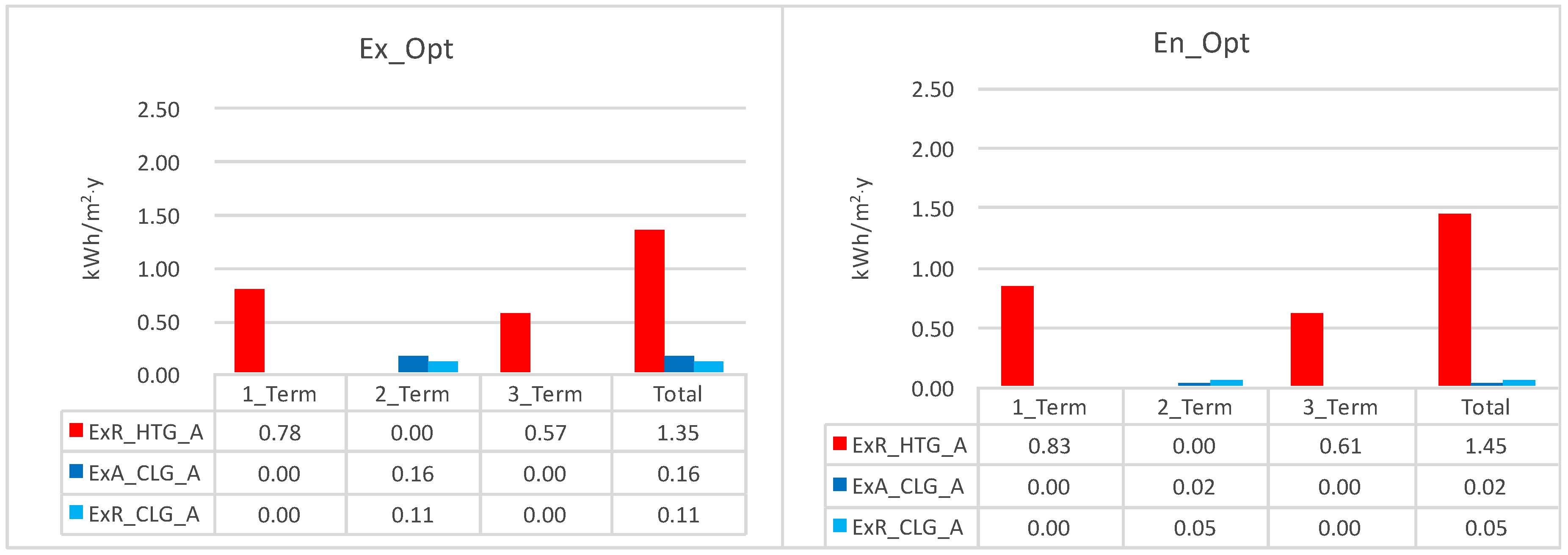
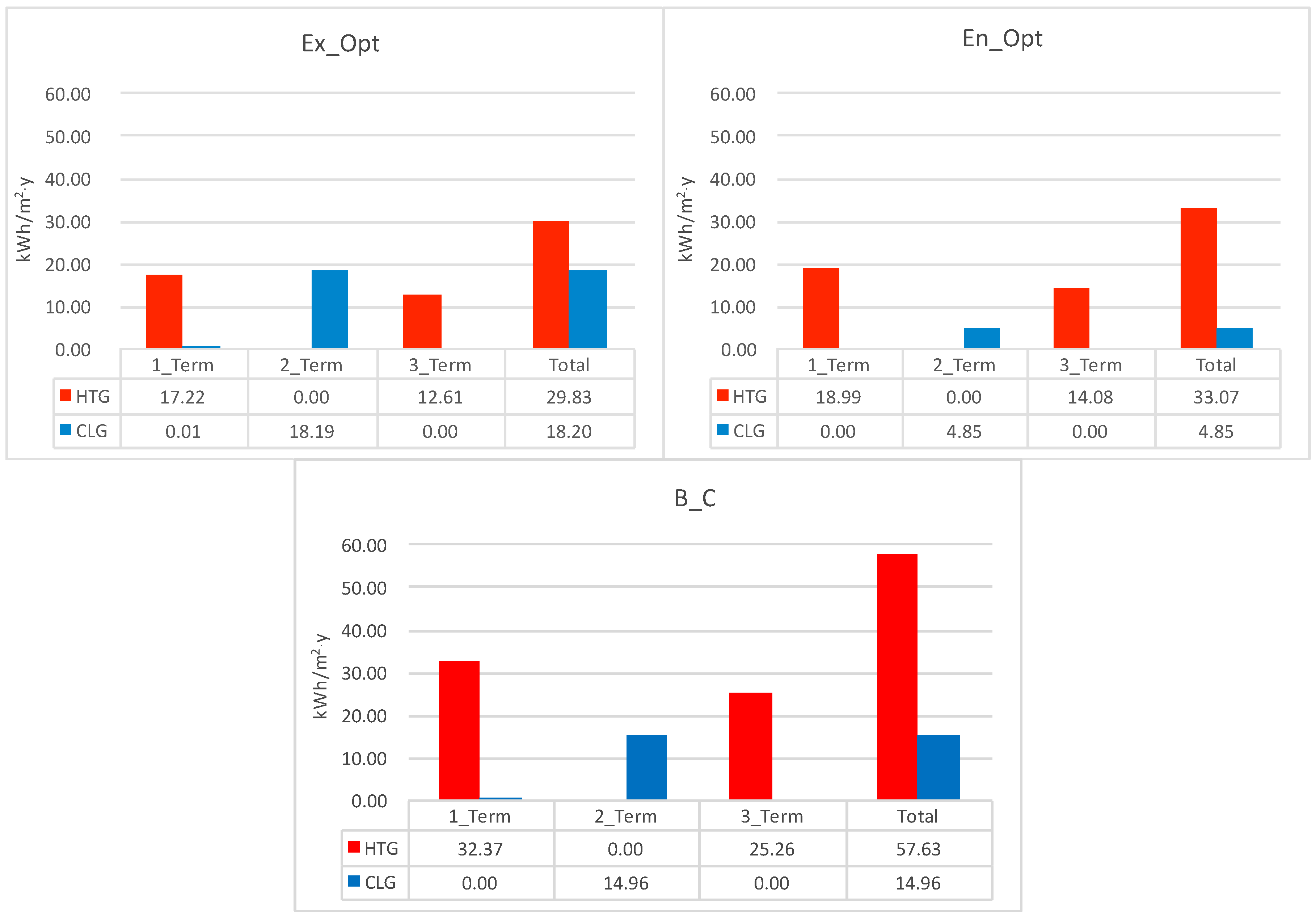
• In the following three graphs, there is no ExA for HTG, because none of the environments can provide that possibility. This means that it is not possible to heat the building with any environment (Figure 6C), because the temperatures are too low to heat the building. This is a logical consequence for this climate in winter. Pamplona has an oceanic climate, Cfb classification according to Köppen. These climates are dominated all year around by the polar front, changeable and often overcast.
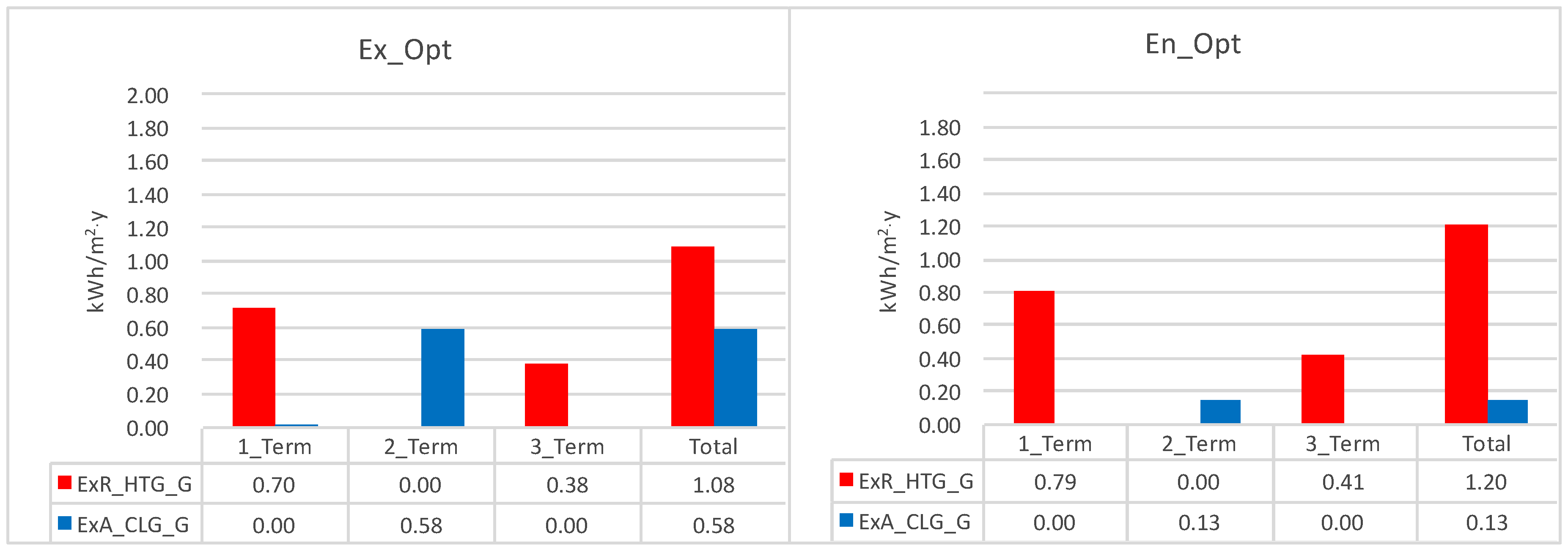
• Both models performed in a similar way with regard to the ExR for HTG, the Ex_Opt model having slightly lower consumption in the three environments. The reason for that is that the envelope configuration in this model is more prone to absorbing solar energy in the winter. However, this effect could vary depending on the weather values from one year to another.
• There is only $Ex{R}_{CLG}$ in the air environment (Figure 12). This means that in this case, it is not possible to cover the cooling needs using the environment according to Figure 6D, and it is necessary to use the schema of Figure 6A to cool the building. As can be seen, the Ex_Opt model maximizes this possibility.
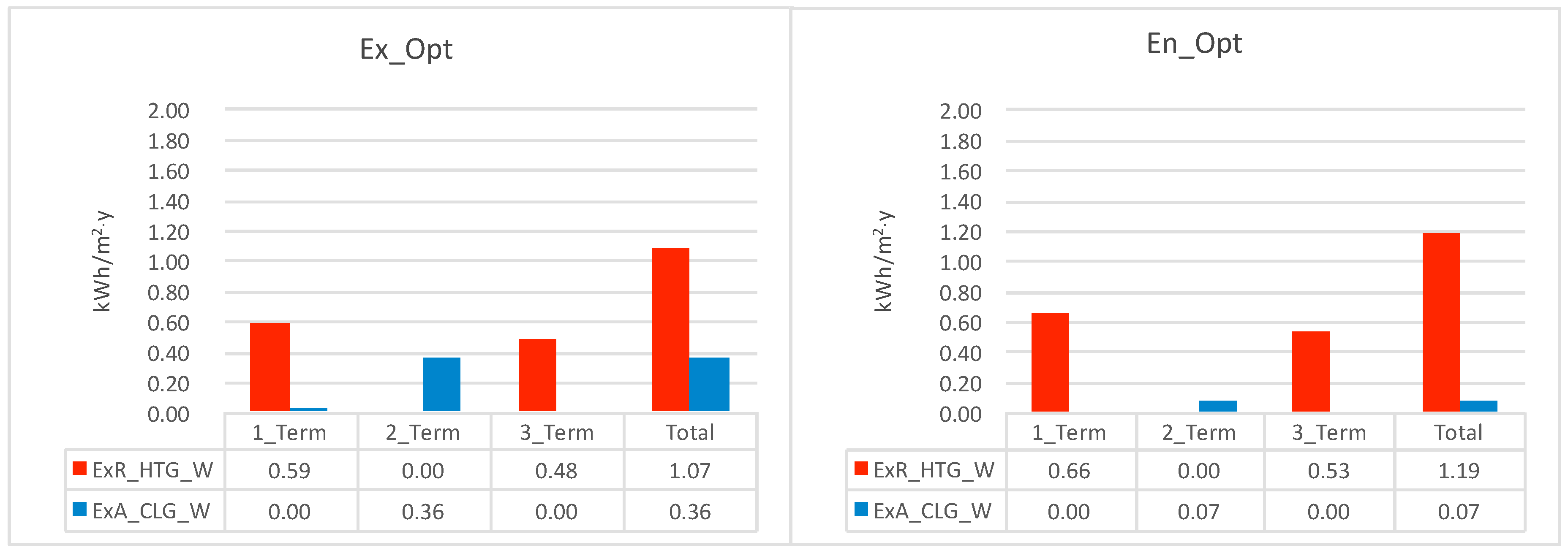
• In Figure 13 and Figure 14, the cooling needs of both models in 2_Term can be totally covered by the environment in accordance with Figure 6D. This is due to the fact that the temperatures of the environment (ground and water) are lower than the set point of the building, as can be seen in Figure 3. In the model Ex_Opt, the building envelope was configured by an objective function, which intends to get as much ExA as possible, and for that reason, in Figure 13 and Figure 14, the use of cooling is higher. This is the main difference between the two types of optimization models.
• All the models have internal temperatures that are within the range of comfort, as can be seen in Figure 3. A special check was made to ensure that the indoor air temperature of any of the models overcame the values proposed by the Spanish health and safety legislation [48].

6. Conclusions

This manuscript has proposed a methodology for applying the simplified exergy demand calculation as expressed in IEA Annex 49 [29] and developed by Schmidt [39] in the dynamic analysis when using detailed building energy models. The main novelty is the development of an internal script for EnergyPlus software that allows classifying the different types of exergy: $Ex{R}_{HTG}$, $Ex{R}_{CLG}$, $Ex{A}_{HTG}$, $Ex{A}_{CLG}$. The classification of each type of exergy has been achieved by considering different environments available in the surroundings of the building. The way the building connects with each environment has been explained in Figure 6. This classification of different exergies solves one of the main problems that occurs when dealing with environments with fluctuating temperatures. This problem obliges one to compute as irreversibilities the difference signs in Equations (3) and (4).

Based on these principles, an optimization process has been done to maximize the possibilities of using the environment in order to extract from it as much exergy as possible. In the case study, the parameters of the building envelope have been modified in order to reach that goal. A unique solution has been reached, and it acts as the best for all three environment conditions. This result is due to the fact that the range of temperature variation of the different environments is very similar. The solution is quite remarkable because the temperature data from the air was taken at an hourly basis, and in the case of the river and the ground, they were taken on a monthly basis. This could mean that the use of dynamic temperature may not be so important, and an average temperature could produce similar results. However, this conclusion should be justified with more case studies.

The optimization results are very consistent, which means that when analysing the ranking of the different models proposed by the algorithm, the components of each type of optimization (energy and exergy) are very similar.

In relation to the materials selected by the models, the windows and skylights have been presented as a quite flexible component in order to give the building different possibilities of consumption and capacity to adapt to the environment. From that point of view and as a specific conclusion, the Ex_Opt model proposes materials (windows glass) of lower quality and therefore is less expensive. In the case of the opaque components, the possibilities for choosing different façades and roofing materials were reduced, but there was a consensus on the selection in both models (Ex_Opt and Ex_En).

In relation to the materials selected by the models, the windows and skylights have been studied, because they are flexible components that lead to different building exergy consumptions and capacity to adapt to the environment. From this specific case study, the conclusion is that the best exergy model indicated that lower quality windows glass be selected. In the case of the opaque components, the possibilities for choosing different façades and roofing materials were reduced; however, there was a consensus on the selection between the best energy model and the best exergy model.

In summary, exergy could be proposed as a sustainable index in the field of retrofitting and specified in the next generation of building energy regulations. It can represent the absolute reduction of CO${}_2$. The manuscript demonstrated that the use of the exergy index could open a space for alternative designs. This is evidenced in the analysis of the differences between the energy and the exergy model. Models that consume less exergy could be more efficient than the models that consume less energy. A greater understanding of this could be achieved with more case studies in the future.

References

1. Mendler, S.; Odell, W.; Lazarus, M.A. The HOK Guidebook to Sustainable Design; Wiley: Hoboken, NJ, USA, 2006. [Google Scholar]
2. Pearce, A.R.; Ahn, Y.H. Sustainable Buildings and Infrastructure: Paths to the Future; Routledge: Abingdon, UK, 2017. [Google Scholar]
3. United Nations. Adoption of the Paris Agreement. 2015. Available online: https://unfccc.int/resource/docs/2015/cop21/eng/l09r01.pdf (accessed on 11 September 2018).
4. Parliament, T.E.; The Council of the EU. Directive 2002/91/EC of the European parliament of the council of 16 December 2002 on the energy performance of buildings. Off. J. Eur. Commun. 2003, L1, 65–71. [Google Scholar]
5. Parliament, T.E.; The Council of the EU. Directive 2010/31/EU of the European parliament and of the council of 19 May 2010 on the energy performance of buildings (recast). Off. J. Eur. Commun. 2010, L153, 13–35. [Google Scholar]
6. Rahmani-Andebili, M. Nonlinear demand response programs for residential customers with nonlinear behavioural models. Energy Build. 2016, 119, 352–362. [Google Scholar] [CrossRef]
7. Rahmani-Andebili, M.; Shen, H. Price-controlled energy management of smart homes for maximizing profit of a GENCO. IEEE Trans. Syst. Man Cybern. Syst. 2017. [Google Scholar] [CrossRef]
8. Rahmani-Andebili, M.; Shen, H. Energy scheduling for a smart home applying stochastic model predictive control. In Proceedings of the 2016 25th International Conference on Computer Communication and Networks (ICCCN), Waikoloa, HI, USA, 1–4 August 2016; pp. 1–6. [Google Scholar]
9. Rahmani-Andebili, M. Scheduling deferrable appliances and energy resources of a smart home applying multi-time scale stochastic model predictive control. Sustain. Cities Soc. 2017, 32, 338–347. [Google Scholar] [CrossRef]
10. Corbin, C.D.; Henze, G.P.; May-Ostendorp, P. A model predictive control optimization environment for real-time commercial building application. J. Build. Perform. Simul. 2013, 6, 159–174. [Google Scholar] [CrossRef]
11. May-Ostendorp, P.; Henze, G.P.; Corbin, C.D.; Rajagopalan, B.; Felsmann, C. Model-predictive control of mixed-mode buildings with rule extraction. Build. Environ. 2011, 46, 428–437. [Google Scholar] [CrossRef]
12. Coffey, B.; Haghighat, F.; Morofsky, E.; Kutrowski, E. A software framework for model predictive control with GenOpt. Energy Build. 2010, 42, 1084–1092. [Google Scholar] [CrossRef]
13. Asadi, E.; da Silva, M.G.; Antunes, C.H.; Dias, L.; Glicksman, L. Multi-objective optimization for building retrofit: A model using genetic algorithm and artificial neural network and an application. Energy Build. 2014, 81, 444–456. [Google Scholar] [CrossRef] [Green Version]
14. Rey, E. Office building retrofitting strategies: Multicriteria approach of an architectural and technical issue. Energy Build. 2004, 36, 367–372. [Google Scholar] [CrossRef]
15. Jaggs, M.; Palmer, J. Energy performance indoor environmental quality retrofit—A European diagnosis and decision making method for building refurbishment. Energy Build. 2000, 31, 97–101. [Google Scholar] [CrossRef]
16. Flourentzou, F.; Roulet, C.A. Elaboration of retrofit scenarios. Energy Build. 2002, 34, 185–192. [Google Scholar] [CrossRef]
17. Gero, J.S.; D’Cruz, N.; Radford, A.D. Energy in context: A multicriteria model for building design. Build. Environ. 1983, 18, 99–107. [Google Scholar] [CrossRef]
18. Schlueter, A.; Thesseling, F. Building information model based energy/exergy performance assessment in early design stages. Autom. Constr. 2009, 18, 153–163. [Google Scholar] [CrossRef]
19. Asadi, E.; da Silva, M.G.; Antunes, C.H.; Dias, L. State of the art on retrofit strategies selection using multi-objective optimization and genetic algorithms. In Nearly Zero Energy Building Refurbishment; Springer: Berlin, Germany, 2013; pp. 279–297. [Google Scholar]
20. Abdel-Salam, M.; El-Dib, A.; Eissa, M. Prediction of ground-level solar radiation in Egypt. Renew. Energy 1991, 1, 269–276. [Google Scholar] [CrossRef]
21. Juan, Y.K.; Kim, J.H.; Roper, K.; Castro-Lacouture, D. GA-based decision support system for housing condition assessment and refurbishment strategies. Autom. Constr. 2009, 18, 394–401. [Google Scholar] [CrossRef]
22. Diakaki, C.; Grigoroudis, E.; Kabelis, N.; Kolokotsa, D.; Kalaitzakis, K.; Stavrakakis, G. A multi-objective decision model for the improvement of energy efficiency in buildings. Energy 2010, 35, 5483–5496. [Google Scholar] [CrossRef]
23. Asadi, E.; Da Silva, M.G.; Antunes, C.H.; Dias, L. Multi-objective optimization for building retrofit strategies: A model and an application. Energy Build. 2012, 44, 81–87. [Google Scholar] [CrossRef]
24. Bonetti, V.; Kokogiannakis, G. Dynamic exergy analysis for the thermal storage optimization of the building envelope. Energies 2017, 10, 95. [Google Scholar] [CrossRef]
25. Crawley, D.B.; Lawrie, L.K.; Winkelmann, F.C.; Buhl, W.F.; Huang, Y.J.; Pedersen, C.O.; Strand, R.K.; Liesen, R.J.; Fisher, D.E.; Witte, M.J.; et al. EnergyPlus: Creating a new-generation building energy simulation program. Energy Build. 2001, 33, 319–331. [Google Scholar] [CrossRef]
26. Klein, S.; Beckman, W.; Mitchell, J.; Duffie, J.; Duffie, N.; Freeman, T.; Mitchell, J.; Braun, J.; Evans, B.; Kummer, J.; et al. TRNSYS 16–A TRaNsient System Simulation Program, User Manual; Solar Energy Laboratory: Golden, CO, USA; University of Wisconsin-Madison: Madison, WI, USA, 2004. [Google Scholar]
27. Crawley, D.B.; Hand, J.W.; Kummert, M.; Griffith, B.T. Contrasting the capabilities of building energy performance simulation programs. Build. Environ. 2008, 43, 661–673. [Google Scholar] [CrossRef] [Green Version]
28. Moran, M.J.; Shapiro, H.N.; Boettner, D.D.; Bailey, M.B. Fundamentals of Engineering Thermodynamics; John Wiley & Sons: Hoboken, NJ, USA, 2010. [Google Scholar]
29. Annex, I.E. 49. Low exergy systems for high-performance buildings and communities. Guideb. Sect. 2010, 6, 1–182. [Google Scholar]
30. Annex, I.E. 37. Low exergy systems for heating and cooling. In Heating and Cooling with Focus on Increased Energy Efficiency and Improved Comfort–Guidebook to IEA ECBCS Annex; VTT: Espoo, Finland, 2004; Volume 37. [Google Scholar]
31. Meggers, F.; Leibundgut, H. The reference environment: Utilising exergy and anergy for buildings. Int. J. Exergy 2012, 11, 423–438. [Google Scholar] [CrossRef]
32. Shukuya, M. Exergy: Theory and Applications in the Built Environment; Springer Science & Business Media: Cham, Switzerland, 2012. [Google Scholar]
33. Mech, R.; Prusinkiewicz, P. Visual models of plants interacting with their environment. In Proceedings of the 23rd ACM Annual Conference on Computer Graphics And Interactive Techniques, New Orleans, LA, USA, 4–9 August 1996; pp. 397–410. [Google Scholar]
34. Pirk, S.; Stava, O.; Kratt, J.; Massih Said, M.A.; Neubert, B.; Mech, R.; Benes, B.; Deussen, O. Plastic trees: Interactive self-adapting botanical tree models. ACM Trans. Gr. 2012, 31, 1–10. [Google Scholar] [CrossRef]
35. Sozer, H. Improving energy efficiency through the design of the building envelope. Build. Environ. 2010, 45, 2581–2593. [Google Scholar] [CrossRef]
36. Yucer, C.T.; Hepbasli, A. Thermodynamic analysis of a building using exergy analysis method. Energy Build. 2011, 43, 536–542. [Google Scholar] [CrossRef]
37. Gonçalves, P.; Gaspar, A.R.; da Silva, M.G. Comparative energy and exergy performance of heating options in buildings under different climatic conditions. Energy Build. 2013, 61, 288–297. [Google Scholar] [CrossRef]
38. Balta, M.T.; Dincer, I.; Hepbasli, A. Performance and sustainability assessment of energy options for building HVAC applications. Energy Build. 2010, 42, 1320–1328. [Google Scholar] [CrossRef]
39. Schmidt, D.; Ala-Juusela, M. Low exergy systems for heating and cooling of buildings. In Proceedings of the 21st Conference on Passive and Low Energy Architecture, Eindhoven, The Netherlands, 19–21 September 2004; pp. 1–6. [Google Scholar]
40. Curzon, F.; Ahlborn, B. Efficiency of a Carnot engine at maximum power output. Am. J. Phys. 1975, 43, 22–24. [Google Scholar] [CrossRef]
41. Bejan, A.; Tsatsaronis, G.; Moran, M. Thermal Design and Optimization; John Wiley & Sons: Hoboken, NJ, USA, 1996. [Google Scholar]
42. İbrahim, D.; Rosen, M.A. Exergy: Energy, Environment, and Sustainable Development. Appl. Energy 2007, 64, 427–440. [Google Scholar]
43. Wepfer, W.; Gaggioli, R. Reference datums for available energy. In Thermodynamics: Second Law Analysis; American Chemical Society: Washington, DC, USA, 1980; Volume 122, pp. 77–92. [Google Scholar]
44. Milne, M. Climate Consultant Software; University of California: Los Angeles, CA, USA, 1991. [Google Scholar]
45. Martín, C.P. Memoria de la Red de Control de Calidad del Agua; Gobierno de Navarra: Pamplona, Spain, 2016; Available online: https://www.navarra.es/NR/rdonlyres/26878783-A91D-4D2F-B392-7E223FDA550A/379051/MEMORIAANUALSAICA2017.pdf (accessed on 10 November 2018).
46. Wall, G.; Gong, M. On exergy and sustainable development-Part 1: Conditions and concepts. Exergy Int. J. 2001, 1, 128–145. [Google Scholar] [CrossRef]
47. Pons, M. On the reference state for exergy when ambient temperature fluctuates. Int. J. Thermodyn. 2009, 12, 113–121. [Google Scholar]
48. De Riesgos Laborales, L.D.P. España. Ley 1995, 31, 8. [Google Scholar]
49. Zhang, Y. Use jEPlus as an Efficient Building Design Optimisation Tool; CIBSE ASHRAE technical symposium: London, UK, 2012; pp. 18–19. [Google Scholar]
50. Ruiz, G.R.; Bandera, C.F.; Temes, T.G.A.; Gutierrez, A.S.O. Genetic algorithm for building envelope calibration. Appl. Energy 2016, 168, 691–705. [Google Scholar] [CrossRef]
51. Deb, K.; Pratap, A.; Agarwal, S.; Meyarivan, T. A fast and elitist multiobjective genetic algorithm: NSGA-II. IEEE Trans. Evol. Comput. 2002, 6, 182–197. [Google Scholar] [CrossRef] [Green Version]
52. Ruiz, G.R.; Bandera, C.F. Analysis of uncertainty indices used for building envelope calibration. Appl. Energy 2017, 185, 82–94. [Google Scholar] [CrossRef]
53. Fernández Bandera, C.; Ramos Ruiz, G. Towards a New Generation of Building Envelope Calibration. Energies 2017, 10, 2102. [Google Scholar] [CrossRef]
Figure 1. Energy supply chain for space climatization in buildings.
Energies 11 03139 g001
Figure 2. Carnot cycle.
Energies 11 03139 g002
Figure 3. Monthly average temperatures for the different scenarios.
Energies 11 03139 g003
Figure 4. Real building vs. model.
Energies 11 03139 g004
Figure 5. (A,B) Skylight in the central area of the building and the brick configuration of the walls. (C) Ducts for air distribution. (D) The Sadar River.
Energies 11 03139 g005
Figure 6. Exergy scenarios: (A) Exergy required for cooling (B) Exergy required for cooling (C) Exergy available for heating (D) Exergy available for cooling.
Energies 11 03139 g006
Figure 7. The script for computing different types of exergy.
Energies 11 03139 g007
Figure 8. Location of the building of School of Architecture of the University of Navarre.
Energies 11 03139 g008
Figure 9. Assembly of the optimization tool.
Energies 11 03139 g009
Figure 10. Best parameters for each component of the envelope.
Energies 11 03139 g010
Figure 11. Energy analysis.
Energies 11 03139 g011
Figure 12. Exergy analysis in the air environment.
Energies 11 03139 g012
Figure 13. Exergy analysis in the ground environment.
Energies 11 03139 g013
Figure 14. Exergy analysis in the water environment.
Energies 11 03139 g014