3.1.1. Steady-State Target Calculation
In this section, we calculate the optimal steady-state targets for the rotor speed
, blade pitch angle
and generator torque
. At a steady-state, we have
Due to less than perfect efficiency, the generator is only able to convert some of the mechanical power to electrical power [
26]. Thus, the objective of maximizing the steady-state electric power
at a given wind speed
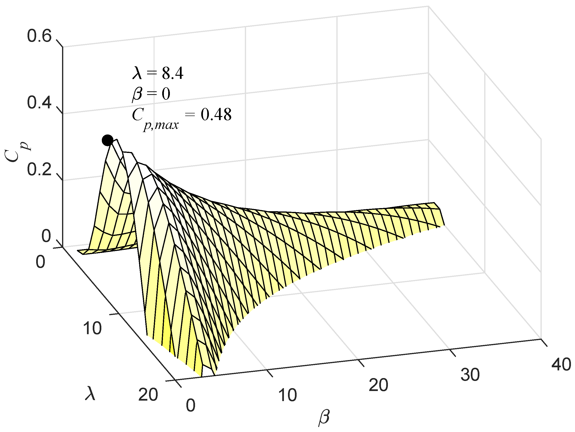
v is equivalent to maximizing the aerodynamic power coefficient
. Note that the dynamics of the generator torque actuator and pitch angle actuator disappear at steady-state conditions. Therefore, we can use the following steady-state optimization problem to find the optimal steady-state operating target:
The above steady-state optimization is a parametric optimization depending on the wind speed
v. The solution is shown in
Figure 5 where the entire operating region is divided into four regions with
, i.e., the cut-in wind speed for WECS,
,
and
as a boundary.
Region IV: When the wind speed is over the rated value (i.e.,
), both the rotor speed and generator torque reaches their upper bound. That is:
WECS keeps the electric power
at its rated value by changing the blade pitch angle as follows:
When the wind speed is below the rated value, the WECS operates in the partial load region which is divided into three subregions, namely, I, II, III as shown in
Figure 5.
Region III: When the wind speed is below the rated value and over the wind speed
(i.e.,
), where
only the rotor speed reaches its upper bound, that is,
The pitch angle is fixed at its optimal value (i.e.,
), and the WECS maximizes electric power
by changing the generator torque as follows:
The classical MPC strategy taken in this work assumes keeping the pitch at its optimal value
before the electrical power reaches its rated value:
Region II: When the wind speed is below the wind speed
and over
(i.e.,
), where
It is expected to maximize wind power capture by maintaining WECS operating at the optimal power coefficient all the time. Previous research results primarily focus on the TSR control in this region, one of the conventional MPPT algorithms. Then, the optimal steady-state is readily obtained as [
11]:
These references in region III and II are also consistent with the optimal steady-state operating target obtained using Equation (
19) in which only constraint Equation (
5) is active in region III.
Region I: When the wind speed is between the cut-in wind speed
and wind speed
(i.e.,
), the rotor angular velocity
is at its lowest allowed value,
and the
reference can be obtained as follows:
In this region, the reference of the pitch angle will be set at the optimal value:
To sum up, the optimal reference rotor angular velocity
, pitch angle
and the generator torque
in MPC design according to the above discussion are as follows:
In the classical tracking MPC design, the MPC will track the three reference trajectories above depending on the wind speed.
3.1.2. Tracking MPC Formulation
The classical tracking MPC for WECS is based on tracking the wind dependent reference trajectories, while minimizing structural fatigue. As stated above, there are different control objectives for different operating regions. The classical tracking MPC achieves this through changing the reference. As for the state constraints of WECS, we will incorporate both hard constraints and soft constraints in the optimization problem. At a sampling time
, the MPC optimization problem for the WECS, under both partial load region and full load region is formulated as follows:
where
denotes the family of continuous piece-wise functions with sampling time
.
N is the predictive horizon.
is the tracking objective function.
is the punishment on slack variables.
is the predicted future state trajectory of the WECS. Equation (
33b) is the nonlinear state-space representation of the WECS in Equation (
18).
in Equation (
33c) is the initial condition at time
. Equation (
33d–h) are the output constraints and state constraints.
The tracking objective function is chosen as:
where
,
,
,
are weights. The first three terms account for wind power capture while the last term of state change rate reflects the structural fatigue of the system.
,
,
are the reference trajectories described in Equation (
32).
The slack variables
,
,
are decision variables associated to the degree of violation of the corresponding constraints. We choose to penalize the slack variables using the quadratic form:
where
is a penalty of the slack variables.
As for the constraints, Equation (
33d–f) mean that the system should remain operating at the rated values when wind speed is over the rated value, while temporary violation of these constraints are acceptable. Treating these constraints as soft constraints makes the MPC optimization problem much easier to solve and may lead to improved closed-loop performance. Equation (
33g) is a constraint on the blade pitch angle and constraints of Equation (
33h,i) impose constraints on the increasing rate of blade pitch angle and the generator torque.
The controller is evaluated at discrete time instants
, with
the initial time and
the sampling time. If we denote the optimal solution to optimization problem Equation (
33) as
, only the first step value of
is applied to the WECS; that is,
At the next sampling time, the MPC optimization problem is re-evaluated.


