A Novel Method for Economic Dispatch of Combined Heat and Power Generation

Abstract

The paper proposes a modified Bat algorithm (MBA) for searching optimal solutions of Economic dispatch of combined heat and power generation (CHPGED) with the heat and power generation from three different types of units consisting of pure power generation units, pure heat generation units and cogeneration units. The CHPGED problem becomes complicated and big challenge to optimization tools since it considers both heat and power generation from cogeneration units. Thus, we apply MBA method with the purpose of enhancing high quality solution search ability as well as search speed of conventional Bat algorithm (BA). This proposed approach is established based on three modifications on BA. The first is the adaptive frequency adjustment, the second is the optimal range of updated velocity, and the third is the retained condition of a good solution with objective to ameliorate the search performance of traditional BA. The effectiveness of the proposed approach is evaluated by testing on 7, 24, and 48 units systems and IEEE 14-bus system and comparing results with BA together with other existing methods. As a result, it can conclude that the proposed MBA method is a favorable meta-heuristic algorithm for solving CHPGED problem.

1. Introduction

Economic dispatch of combined heat and power generation (CHPGED) plays an important role in modern power systems. Thus, many researchers have constantly developed its problem formulation and applied different optimization tools for solving such problems. The fuel cost is comprised of heat generation and power generation in which heat from electricity generation process is retained and transmitted to heat loads such as industrial zones and manufacturers as well as for other aims [1]. In combined heat and power systems, pure power generation units and cogeneration units are in charge of providing electricity to electric loads while pure heat generation units and cogeneration units undertake heat generation and heat transmission to heat loads. In general, the operating enhancement of pure power plants is much simpler than that of cogeneration plants; that is because of the complicated output characteristics of a cogeneration plant. In practice, the energy generation characteristics of pure plants are a fuel cost function. For pure plants, this function is either only heat or power output. Meanwhile cogeneration plants comprise both heat and power outputs which shows that the operating range of cogeneration plants is more complicated. Therefore, the CHPGED issue is a major challenge for the optimization tools for finding optimal solutions satisfying all constraints exactly and reducing total fuel cost effectively.

Over several decades, the authors in [2,3,4,5,6,7] have introduced different methods to solve the CHPGED. The Newton [2] and Lagrange relaxation (LR) [3] methods are two of those methods that were first applied to solve the CHPGED issue. However, they have a common main disadvantage of being limited when dealing with a large-scale system. In order to overcome this disadvantage, the authors in [4] have proposed the combined method between the augmented Lagrange and Hopfield network (ALHN). As a result, a very good solution with a short computation time is obtained. In order to reduce the number of iterations and the loop time by speeding up the computation, the authors of [5] have presented the novel direct search (NDS) method based on a successive refinement search technique. The Newton method and other methods such as ALHN and NDS can solve nonlinear constrained optimization problems but Lagrange relaxation (LR) cannot deal with the issue. Thus, ref. [6] has proposed the combination of sequential quadratic programming (SQP) and LR, called SQP-LR method. In the method, SQP could solve nonlinear constraints successfully while LR could find optimal solution satisfying all remaining constraints. Unlike SQP-LR, meta-heuristic algorithms can solve non-linear problems simply and successfully although they do not need to use SQP method. LR with surrogate sub-gradient technique (LR-SST) [7] has been developed by using the main search function of LR and the updating function of SST. LR has also been used for the same purpose as the methods in [3,6] while SST has been used to calculate the values of Lagrange multipliers automatically. Compared to LR, LR-SST was more effective for applications because selection of Lagrange multipliers was no longer an issue in LR-SST. However, LR-SST and other methods in the conventional method group have the same main disadvantage of impossibility of solving CHPGED problem considering valve point loading effects, which is represented as non-convex fuel cost function form.

A number of studies [8,9,10,11,12,13,14,15,16,17,18,19] have used meta-heuristic algorithms based on random search considering the non-convex objective issue for the CHPGED. Among those, the authors in [8] have proposed a method that is a combination of the modified genetic algorithm (AG) and penalty function trials. However, this method may be only trapped at a local optimal solution when varying a wide range of the penalty factors. To have a better result compared to the method proposed in [8], the authors of [11] have improved AG with multiplier updating by applying an augmented Lagrange optimization function and penalty method. Nonetheless, their method converged slowly to a satisfactory optimal solution. The evolutionary programming (EP) method has been introduced in [10]. However, this method has two disadvantages, namely its slow convergence and easily falling into a local optimum. The self-adaptive real-coded genetic algorithm has been introduced in [13], in which a new selection and crossover has been carried out on real-coded GA. As result, this method has good convergence. Using the harmony search (HS) for the CHPGED, the authors in [15,16] have proposed to modify it, and the obtained results are significantly improved. However, its convergence tool takes a long time to approach the optimal solutions. Using the particle swarm optimization (PSO) algorithm for the CHPGED, a new method [12] was developed on PSO by suggesting the use of the maximum velocity and selection operations. However, the obtained results are not very good compared to the methods in [8,11]. The time-varying acceleration factors are introduced in addition to the time-varying inertia weight coefficients in PSO to modify two acceleration factors on PSO with a constriction coefficient, so that the optimal solution can be enhanced. On the other hand, a new method in [19] has been developed by modifying the group search optimization (GSO). In this case, the obtained result showed that the requested run time is very long when studying a large-scale system. Moreover, the CHPGED considering the valve point loading effects on pure power units has been sufficiently solved by the bee colony optimization (BCO) in [14]. The obtained results are better than EP and PSO under conditions of the optimum value and computation time. However, the major restriction of this method is the application for large-scale power systems because it has taken long simulation time for a seven-unit system but gives a low quality solution. Similarly, the CHPGED is solved based on the artificial immune system (AIS) method. The objective is to obtain the optimal solution by using of few control parameters and a small number of iterations. However, the disadvantage of this method is the ability to suffer premature convergence when applying the aging operator to eliminate the bad antibodies.

In recent years, some most promising methods have proposed for the CHPGED, like the group search optimization [20], oppositional teaching learning based optimization [21], opposition-based group search optimization [22], and eight versions of PSO [23], grey wolf optimization [24], machine learning algorithm [25], and the cuckoo search algorithm [26]. It is observed that the performance of these methods seems to be better than all the methods given in [8,9,10,11,12,1314,15,16,17,18,19] for most cases.

This paper proposes a pertinent method for solving the CHPGED on the basis of the Bat algorithm (BA), considering three modifications that are the adaptive tuning frequency, optimal range of updated velocity, and retained condition of a good solution with the purpose to improve the searching performance of conventional BA. To verify the effectiveness of the proposed method, several simulation cases of the proposed method and conventional BA are analyzed based on four test case with a 7-unit system, 24-unit system, 48-unit system and an IEEE 14-bus system. In addition, transmission power losses, non-differential objective function and all constraints of transmission power networks have been taken into consideration. The main new contributions of this paper are summarized as follows:

(i)

Conventional BA is first applied for solving the CHPGED and

(ii)

Pointing out drawbacks of BA and suggesting modifications on conventional BA to develop modified Bat algorithm with better performance.

The remainder of this paper is organized as follows. Section 2 covers the methodologies for the CHPGED problem while Section 3 gives the proposed algorithm for CHPGED. Case study, simulation results, and discussion of the results are handled in Section 4 and Appendix A. Finally, conclusions are reported in Section 5.

2. Methodologies

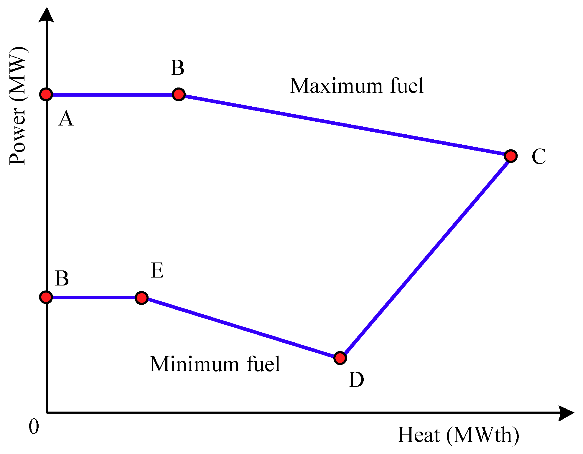
Suppose that we have a complex power system that includes the pure power generation units N_pp, pure heat generation units N_ph, and cogeneration units N_c. Here, the main objective of the CHPGED is to minimize total fuel cost of heat generation and electricity generation from available generation units. To reach the objective, the main duty is to determine heat output of cogeneration units and pure heat generation units, and power output of cogeneration units and pure power generation units. In addition, constraints of working limitations from all generation units, power balance and heat balance must be exactly satisfied. Especially, the relationship between heat and power outputs of a cogeneration units shown in Figure 1 is really complex.

Figure 1 is an example of the feasible operating zone of a cogeneration unit. Figure 1 is depicted by using given data of heat outputs and power outputs of a typical cogeneration unit in which the efficiency of the unit cannot be known as observing the figure but its performance can be evaluated by using a fuel cost function. The observation from Figure 1 in [27] and Figure 5 in [28] can indicate that efficiency of the cogeneration unit is complicated for calculation. In fact, the efficiency is directly influenced by thermal efficiency and heat efficiency, and it is also related to power output and heat output. Simulation results from [29] also indicate the same statement, since points of efficiency are not a mathematical function. In our work, we suppose that feasible operating zone and fuel cost function of cogeneration units are exactly given by taking data from previous studies. Our main task is to determine power and heat outputs so that the values must be inside the feasible operating zone and the fuel cost can be reduced as much as possible.

2.1. Cost Objective Function

For the objective of the CHPGED issue, we consider a minimum cost objective function of the heat and electricity power production under the following form:

$$\mathrm{Min}\left\{{\displaystyle \sum _{i=1}^{N_{pp}}{F}_{pi}(P_{pi})}+{\displaystyle \sum _{j=1}^{N_c}{F}_{cj}(P_{cj},H_{cj})}+{\displaystyle \sum _{k=1}^{N_{ph}}{F}_{hk}(H_{hk})}\right\},$$

(1)

The cost functions of the pure power generator i for the case of neglecting and considering valve point loading effects are respectively mathematically formulated in Equations (2) and (3) [14]:

$$F_{pi}(P_{pi})=a_{pi}+b_{pi}{P}_{pi}+c_{pi}{P}_{pi}^2$$

(2)

$$F_{pi}(P_{pi})=a_{pi}+b_{pi}{P}_{pi}+c_{pi}{P}_{pi}^2+\left|e_{pi}\times \sin (f_{pi}\times (P_{pi}^{\min }-P_{pi}))\right|$$

(3)

The cost objective function of the kth pure heat generator can be calculated as follows [17]:

$$F_{hk}(H_{hk})=a_{hk}+b_{hk}{H}_{hk}+c_{hk}{H}_{hk}^2,$$

(4)

The cost objective function of the jth cogeneration unit can be calculated as follows [17]:

$$F_{cj}(P_{cj},H_{cj})=a_{cj}+b_{cj}{P}_{cj}+c_{cj}{P}_{cj}^2+k_{cj}{H}_{cj}+l_{cj}{H}_{cj}^2+m_{cj}{H}_{cj}{P}_{cj},$$

(5)

where P_pi and P_cj are the power output of the ith pure power generation unit and jth cogeneration unit, respectively; H_cj and H_hk the heat output of the j-th cogeneration unit and heat output of the kth pure heat generation unit, respectively; a_pi, b_pi, c_pi, e_pi and f_pi are the pure electricity generation cost function coefficients of the ith pure power generation unit; a_hk, b_hk and c_hk are the pure heat generation cost function coefficients of the kth pure heat unit; and a_cj, b_cj, c_cj, k_cj, l_cj and m_cj are the heat and electricity generation cost function coefficients of the jth cogeneration unit. Among the definitions, values of power outputs and heat outputs are determined by operators in power plants while coefficients in all cost functions are predetermined by experts in power plants by conducting experiments on the units.

2.2. Constraints

2.2.1. Active Power balance

The active power generated by pure power and cogeneration units must be equal to the active power demand of power systems, and can be considered as follows:

$$P_D+P_L-{\displaystyle \sum _{i=1}^{N_{pp}}{P}_{pi}}-{\displaystyle \sum _{j=1}^{N_c}{P}_{cj}}=0,$$

(6)

where P_D is the power demand and P_L is the loss power in the transmission line, and can be calculated as follows [14,17]:

$$P_L={\displaystyle \sum _{i=1}^{Npp+Nc}{\displaystyle \sum _{j=1}^{Npp+Nc}{P}_i{B}_{ij}{P}_j}}+{\displaystyle \sum _{i=1}^{Npp+Nc}{B}_{0i}{P}_i}+B_{00}.$$

(7)

2.2.2 Heat balance

The produced total heat due to the pure heat and cogeneration units must satisfy the heat demand and neglect heat loss, and can be considered as follows:

$$H_D-{\displaystyle \sum _{j=1}^{N_c}{H}_{cj}}-{\displaystyle \sum _{k=1}^{N_{ph}}{H}_{hk}}=0,$$

(8)

In the constraint, heat losses are supposed to be zero because there have not been any studies about heat losses during process of transmitting heat to heat loads. In the work, we have also used that assumption for simplicity. However, if heat losses are a function of heat outputs similar to power loss function or a constant, heat balance constraint will be solved simply and successfully.

2.2.3. Power and heat unbalance

Each generation unit must operate within its upper and lower limit. The power of ith pure power, jth cogeneration, and the kth pure heat and the jth cogeneration units can be expressed, respectively, as follows:

$$P_{pi}^{\min }\le P_{pi}\le P_{pi}^{\max },$$

(9)

$$P_{cj}^{\min }(H_{cj})\le P_{cj}\le P_{cj}^{\max }(H_{cj}),$$

(10)

$$H_{cj}^{\min }(P_{cj})\le H_{cj}\le H_{cj}^{\max }(P_{cj}),$$

(11)

$$H_{hk}^{\min }\le H_{hk}\le H_{hk}^{\max },$$

(12)

in which, the limit functions of power output of the j-th cogeneration unit can be calculated as follows:

$$P_{cj}^{\max }(H_{cj})=\min \left\{{P_{cj}(H_{cj})|}_{AB},{P_{cj}(H_{cj})|}_{BC}\right\},$$

(13)

$$P_{cj}^{\min }(H_{cj})=\max \left\{{P_{cj}(H_{cj})|}_{CD},{P_{cj}(H_{cj})|}_{DE},{P_{cj}(H_{cj})|}_{EF}\right\},$$

(14)

the limit functions of heat outputs of the j-th cogeneration unit can be calculated as follows:

$$H_{cj}^{\max }(P_{cj})=\min \left\{{H_{cj}(P_{cj})|}_{BC},{H_{cj}(P_{cj})|}_{CD}\right\},$$

(15)

$$H_{cj}^{\min }(P_{cj})=0.$$

(16)

2.3. Slack Units

In this paper, two slack variables including the slack pure power P_p1 and the slack pure heat generation unit H_h1 are considered to exactly meet the balance constraints of power and heat:

2.3.1. Pure Power Generation Unit

Suppose that the power outputs of (N_pp −1) pure power generation units and N_c cogeneration units are known. The power output of the first pure power generation unit can be calculated using Equation (6) as follows:

$$P_{p1}=P_D+P_L-{\displaystyle \sum _{i=2}^{N_{pp}}{P}_{pi}}-{\displaystyle \sum _{j=1}^{N_c}{P}_{cj}},$$

(17)

where P_L can be calculated by using Equation (7).

2.3.2. Pure Heat Generation Unit

The slack pure heat generation unit H_h1 is considered using Equation (8) according to the known heat outputs of other pure heat and cogeneration units as:

$$H_{h1}=H_D-{\displaystyle \sum _{j=1}^{N_c}{H}_{cj}}-{\displaystyle \sum _{k=2}^{N_{ph}}{H}_{hk}}.$$

(18)

3. Algorithms

3.1. Conventional Bat Algorithm

The Bat algorithm was developed in 2010 derived from the behavior of bat species during their food search [30]. The main rules of the BA method can be summarized as follows:

(i) 

Each Bat d has a position X_d and a velocity V_d, and it generates a pulse with the frequency f_d, the loudness A_d, and the rate r_d as well.

(ii) 

The loudness A_d generated by a Bat gets the largest value at the beginning of the search process, reduces gradually, and then reaches the lowest one as approaching to its prey.

Each Bat’s position is the indices of a solution of optimization problems, which will be gradually enhanced while the number of iterations is increased, and the velocity is used to determine the following positions emblematizing the possibility of changing positions of a Bat. Increasing the number of iterations, normally, the searching process could generate a new position which would be closer to the food source than the previous positions. It means that the quality of a new solution tends to be better than that of the previous solution. To generate new positions, search space around each old solution, called global search and search space around the best solution in the population, called local search are carried out. Basic steps of BA can be summarized in detail as bellow.

Given a set of N_B Bats, calling $X_d^G$ and $V_d^G$ are the current position and velocity of the dth Bat in the population, d = 1, 2, …, N_B.

At the beginning of each iteration step, the frequency of each Bat can be randomly initialized as:

$$f_d^G=f_{\min }+rand.(f_{\max }-f_{\min }),$$

(19)

and, the new velocity and position of each Bat are:

$$V_d^G=V_d^{G-1}+f_d^G\left(X_d^{G-1}-X*\right),$$

(20)

$$X_d^G=X_d^{G-1}+V_d^G,$$

(21)

where X* is the best position among N_B Bats in a population. This solution is determined from the random positions of the initial population for the first iteration and chosen from existing population at the end of each iteration.

For a local search, each Bat has a chance to generate a new position which is around the best location, can be described as follows:

$$X_{d,new}^{}=X*+\mathsf{\epsilon }{A}_{}^G,$$

(22)

where ε is a random number selected in range [0, 1], and A^G is the average loudness of all Bats.

In fact, the loudness and pulse emission rate of each Bat are not fixed values, but they should be rapidly changed as the Bat moves around its prey. It means that once the Bat has discovered a prey, its loudness tends to decreases meanwhile the pulse emission rate increases. As a result, the updated loudness and rate are determined as:

$$A_d^{G+1}=\mathsf{\alpha }{A}_d^G,$$

(23)

$$r_d^{G+1}=r_d^G\left[1-\exp (-\mathsf{\gamma }G)\right],$$

(24)

in which the coefficients α and γ are arbitrary values in range [0, 1], and kept constant during the search process. In the studies [30,31,32], the two parameters were set to the same value of 0.9 for simplicity, but they should be dependent on the specific applications by experiment. However, analyzing Equation (24), we can see that the pulse emission rate does not increase if the γ is set to 0.9, and the probability for local search is not higher during the search process.

The BA’s pseudo code was described in detail in [30]. The BA has been more advanced than other algorithms in terms of accuracy and efficiency for many test functions [30] as well as successfully applying for simple cases of optimal operation of power systems [33,34]. However, to deal with more complex problems, some modifications have been suggested in the variants of the BA as mentioned in [35].

3.2. Modified Algorithm

In order to improve the searching performance of the BA for solving the CHPGED, in this paper, we propose three new modifications, including adaptive tuning frequency, the optimal range of updated velocity, and new criteria of competitive solutions. The three modifications can be summarized as follows:

3.2.1. Adaptive Frequency Adjustment Corresponding to the Number of Iterations

In the BA, at each iteration, the frequency is randomly produced within its operating frequency range as defined in Equation (19). As a result, an updated velocity generated arbitrarily as defined in Equation (20) could be over-speeded and make the Bat fly away from the optimal point. This problem is more serious at higher iterations where the Bats are closely approached to the prey. In the optimization point of view, at higher iterations when a Bat is nearly reach to the prey, this Bat’s flying speed must be slowed down and the movement should be just around the current position (neighboring areas of the prey’s location). Thus, by experiment, we suggest that at each iteration, the updated frequency should be adjusted as:

$$\begin{array}{cc}\hfill f_d^G& =\frac{(G_{\max }-G)}{G_{\max }}{f}_d^{G-1}\hfill \\ & =f_d^{G-1}-\frac{G}{G_{\max }}{f}_d^{G-1}\hfill \end{array}$$

(25)

In Equation (25), our intention is to reduce the frequency gradually according to the increase of iteration. As the iterations increase, the frequency decreases. On the other hand, the new velocity obtained from Equation (20) and new position calculated from Equation (21) are also narrowed as the iteration increases because the velocity is proportional to the frequency and the position is proportional to the velocity. It is clear that the search space is exploited in large ranges at the beginning of the search process but it contracted as the iterations increase to the maximum value.

3.2.2. Set the Optimal Range of the Updated Velocity

The velocity is one main factor used to update new position for each Bat. If the velocity is high, the Bats’ positions, i.e., solutions could move the feasibility area outside whereas the small velocity could limit the discovery areas. For the BA, there is no information discussing the optimal range of velocity, while this term has been constantly improved in PSO [23]. In [23], authors have mentioned that the optimal range of the velocity can be fixed from 10% to 15% of the difference between the boundary positions. For this study, we suggest that the updated velocities of the Bats should be narrowed in a range of $\left[V_d^{\min },V_d^{\max }\right]$, where:

$$V_d^{\max }=0.15(X_d^{\max }-X_d^{\min }),$$

(26)

$$V_d^{\min }=-V_d^{\max },$$

(27)

and $X_d^{\max }$ and $X_d^{\min }$ are the maximum and minimum positions in the searching area, respectively.

3.2.3. Define New Criteria of Competitive Solutions

In the BA, a new solution is retained only if both conditions are satisfied, that is its fitness function is smaller than that of the old solution (of the same Bat) and its assigned random value is equal to or lower than the current loudness [30,31,35]. The selection technique of BA can expressed by the following Algorithm 1.

Algorithm 1. Selection technique of BA

$$\begin{gathered} If\left(F{F}_{d,new}\le F{F}_d\right)\&\left(ran{d}_d^{}\le A_d^G\right) \\ {X}_{d,new}=X_{d,new}\&A_d^{G+1}=\mathsf{\alpha }{A}_d^G \\ \mathrm{else} \\ {X}_{d,new}=X_{d,new}\&A_d^{G+1}=A_d^G \\ \mathrm{end} \end{gathered}$$

In the algorithm, if the two conditions are true, the loudness $A_d^G$ becomes much smaller than the previous value because α is fixed at 0.9 and the possibility that better solution is kept to be low. Thus, we suggest that the loudness should be set to 1 at the beginning and afterwards decreased by a very small step size as shown in Equation (28):

$$\begin{array}{cc}\hfill A_d^G& =\frac{G_{\max }-\sqrt{G}}{G_{\max }}\hfill \\ & =1-\frac{\sqrt{G}}{G_{\max }}\hfill \end{array}$$

(28)

The equation can increase the value of $A_d^G$ compared to that of Equation (23), giving an opportunity for the use of a new solution with a better fitness function and replacement of old solutions with worse fitness functions.

The proposed modified bat algorithm (MBA) has been applied for a complex optimal power system operation problem where the combined heat and power outputs have been closely related together. In this problem, the power system was supplied by many kinds of the normal thermal generators and cogeneration sources.

3.3. Application

In CHPGED problems, a power system is supplied by N_pp pure power generation units, N_ph pure heat generation units and N_c cogeneration units. Similar to other meta-heuristic algorithms, the proposed MBA needs a set of Bats N_B where each Bat has its own velocity and position. The position of the Bat dth, called X_d (d = 1 ÷ N_B), is a solution of the problem containing power outputs of (N_pp−1) pure power units and heat outputs of (N_ph-1) pure heat generation units together with heat and power outputs of N_c cogeneration units. 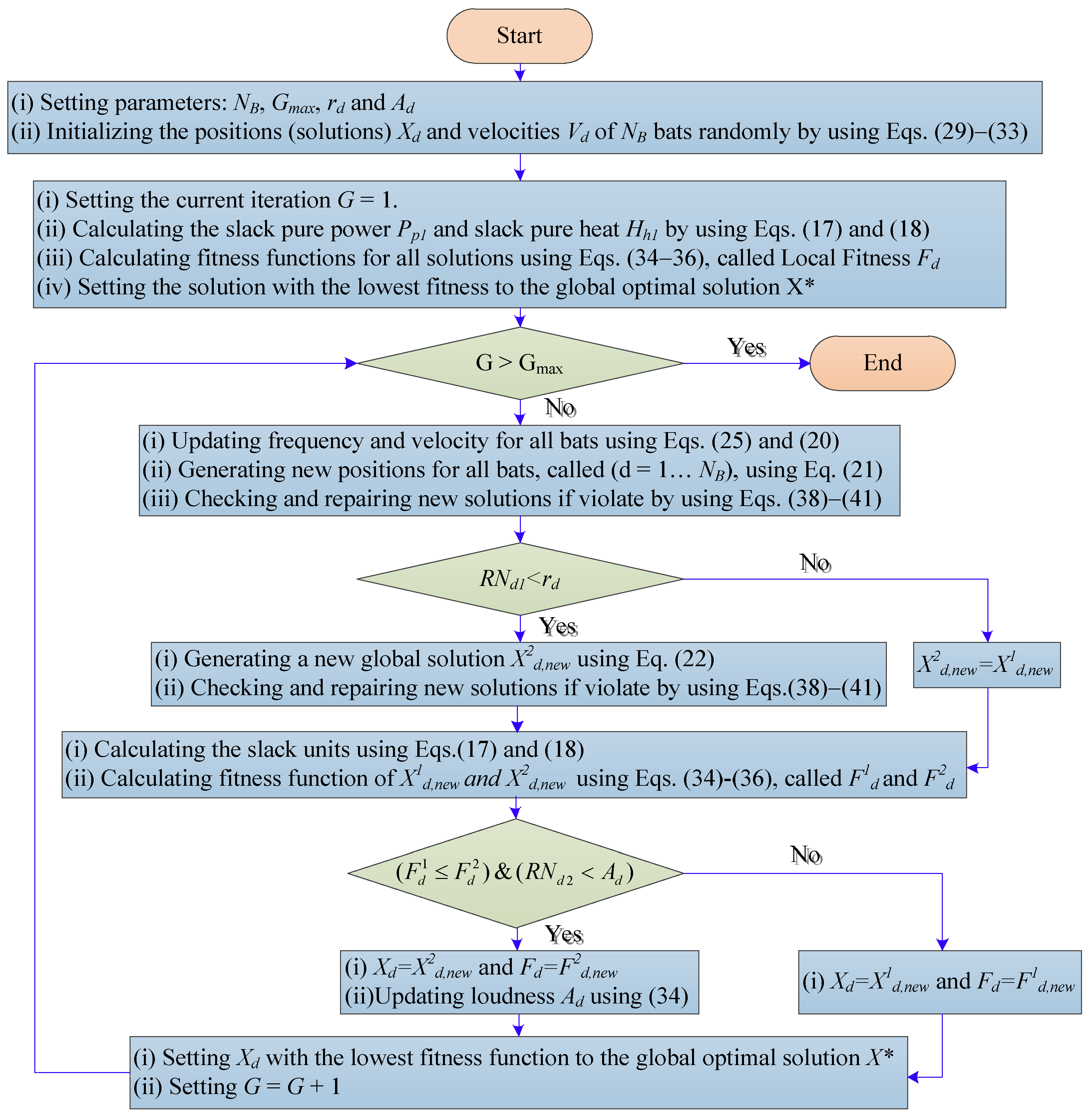The maximum iterations are fixed at beginning and the position of Bats (solutions) N_B will be updated time by time after each iteration. The search process- based MBA will guide the Bats moving toward the prey (the optimal solution) quickly and stably as shown in the following steps. The flowchart for solving the CHPGED is presented in Figure 2.

Step 1: Initialization of the whole population

The initialization is implemented as follows:

$$P_{pi,d}=P_{pi}^{\min }+rand(P_{pi}^{\max }-P_{pi}^{\min });i=2,...,N_{pp},$$

(29)

$$P_{cj,d}=P_{cj}^{\min }+rand(P_{cj}^{\max }-P_{cj}^{\min });j=1,...,N_c,$$

(30)

$$H_{cj,d}=H_{cj}^{\min }+rand(H_{cj}^{\max }-H_{cj}^{\min });j=1,...,N_c,$$

(31)

$$H_{hk,d}=H_{hk}^{\min }+rand(H_{hk}^{\max }-H_{hk}^{\min });k=2,...,N_{ph}.$$

(32)

The velocity of each Bat is initialized as:

$$V_{d,}=V_d^{\min }+rand(V_d^{\max }-V_d^{\max });d=1,...,N_B.$$

(33)

where $V_d^{\max }$, $V_d^{\min }$ are obtained by applying the second modification, Equations (26) and (27), respectively.

From the initialized values of N_B Bats, the fitness function corresponding to the position of each Bat is calculated as follows:

$$\begin{array}{cc}\hfill FT(X_d)={\displaystyle \sum _{i=1}^{N_{pp}}{F}_{Pi}(P_{pi,d})}& +{\displaystyle \sum _{j=1}^{N_c}{F}_{cj}(P_{cj,d},H_{cj,d})}+{\displaystyle \sum _{k=1}^{N_{ph}}{F}_{hk}(H_{hk,d})}\hfill \\ & +K_p{(P_{p1,d}-P_{p1}^{\lim })}^2+K_h{(H_{h1,d}-H_{h1}^{\lim })}^2.\hfill \end{array}$$

(34)

where P_p1,d nd H_h1,d are the power and heat output of the slack pure power and pure heat generation units of the d-th solution, obtained from Equations (17) and (18), respectively; and K_p and K_h are penalty coefficients for the power and heat outputs of those slack generation units, respectively.

The limits of the slack generation units $P_{p1}^{\lim }$ and $H_{h1}^{\lim }$ in Equation (34) are determined as follows:

$$P_{p1}^{\lim }=\{\begin{array}{cc}{P}_{p1}^{\max }& \mathrm{if}{P}_{p1,d}>P_{p1}^{\max }\\ P_{p1}^{\min }& \mathrm{if}{P}_{p1,d}<P_{p1}^{\min }\\ P_{p1,d}& \mathrm{otherwise}.\end{array}$$

(35)

$$H_{h1}^{\lim }=\{\begin{array}{cc}{H}_{h1}^{\max }& \mathrm{if}{H}_{h1,d}>H_{h1}^{\max }\\ H_{h1}^{\min }& \mathrm{if}{H}_{h1,d}<H_{h1}^{\min }\\ H_{h1,d}& \mathrm{otherwise}.\end{array}$$

(36)

Note that $P_{p1}^{\max }$ and $P_{p1}^{\min }$ are the maximum and minimum power generations of the slack power generation unit, which must be similar to the limits of other pure power generation units. $H_{h1}^{\max }$ and $H_{h1}^{\min }$ are the maximum and minimum heat productions of the slack heat generation unit to be similar to the the limits of other pure heat generation units.

Among all initialized members, the Bat’s position with the lowest value of fitness functions is assigned as the global best position (solution), X^*.

Step 2: Update New Velocity and Position for Each Bat

In this proposed method, each Bat has a position and a velocity where the position represents a solution and the velocity represents an updated step size for a new position. Therefore, the value of the velocity has an impact on the obtained solution while the value of current frequency also plays a very important role to generate an effective velocity. The adaptive frequency $f_d^G$ is caculated from Equation (25) and the each Bat velocity is updated by applying Equation (20).

Furthermore, the new velocity needs to be checked by the optimal range of the velocity as mentioned in Equations (26) and (27). The constraint for this velocity can be described by:

$$V_d=\{\begin{array}{l}{V}_d^{\max }\mathrm{if}{V}_d>V_d^{\max }\\ V_d^{\min }\mathrm{if}{V}_d<V_d^{\min }\\ V_d\mathrm{otherwise}\end{array};d=1,...,N_B,.$$

(37)

and a new position of each Bat related to the new velocity is determined from Equation (21).

Step 3: Search a New Solution

As described in the conventional BA [30,35], there is a possibility that a current X_d can be newly produced around the current global best solution by applying Equation (22) if its random value is less than the pulse rate r_d, within range [0,1]. This r_d is set to a specific value at the beginning of the search process and increased during the following iterations. Obviously, if the r_d is set to at a high value equal to 1, almost all new solutions are nearby the current global best solution and the final optimal solution may possibly fall in a local optimal value. Inversely, few solutions could be newly generated that can be nearby the global best solution if the r_d is set to a very low value. Each specific optimization problem should be existed a suitable range of the pulse rates depending on its characteristics. Therefore, in order to discover the suitable, the pulse rates of the MBA for the CHPGED problem will be carried out by varying within range [0, 1] with a step of 0.1.

The new solutions need to be checked whether they satisfy their limits, which are mentioned in Equations (9)−(12), by using the following models:

$$P_{pi,d}=\{\begin{array}{l}{P}_{pi}^{\max }\mathrm{if}{P}_{pi,d}>P_{pi}^{\max }\\ P_{pi}^{\min }\mathrm{if}{P}_{pi,d}<P_{pi}^{\min }\\ P_{pi,d}\mathrm{otherwise}\end{array};i=2,...,N_{pp}$$

(38)

$$P_{cj,d}(H_{cj,d})=\{\begin{array}{l}{P}_{cj}^{\max }(H_{cj,d})\mathrm{if}{P}_{cj,d}(H_{cj,d})>P_{cj}^{\max }(H_{cj,d})\\ P_{cj}^{\min }(H_{cj,d})\mathrm{if}{P}_{cj,d}(H_{cj,d})<P_{cj}^{\min }(H_{cj,d})\\ P_{cj,d}(H_{cj,d})\mathrm{otherwise}\end{array};j=1,...,N_c$$

(39)

$$H_{cj,d}(P_{cj,d})=\{\begin{array}{l}{H}_{cj}^{\max }(P_{cj,d})\mathrm{if}{H}_{cj,d}(P_{cj,d})>H_{cj}^{\max }(P_{cj,d})\\ H_{cj}^{\min }(P_{cj,d})\mathrm{if}{H}_{cj,d}(P_{cj,d})<H_{cj}^{\min }(P_{cj,d})\\ H_{cj,d}(P_{cj,d})\mathrm{otherwise}\end{array};j=1,...,N_c$$

(40)

$$H_{hk,d}=\{\begin{array}{l}{H}_{hk}^{\max }\mathrm{if}{H}_{hk,d}>H_{hk}^{\max }\\ H_{hk}^{\min }\mathrm{if}{H}_{hk,d}<H_{hk}^{\min }\\ H_{hk,d}\mathrm{otherwise}\end{array};k=2,...,N_{ph}$$

(41)

The power of the slack power generation unit and the heat of the slack heat generation unit can be calculated by using Equations (17) and (18), and can be checked by applying Equations (35) and (36), respectively.

Step 4: Find New Solution through the New Criteria of Competitive Solutions

The current solutions are evaluated through the calculation of the fitness functions, and then the selection of between the current and the initialized solutions) is decided according to the last modification in Section 3.2. We update the new loudness A_d according to the current number of iterations G as shown in Equation (28).

4. Case Study and Discussion

In the section, four study cases with different numbers of units, constraints and objective functions are carried out for investigating the performance of MBA. The description of the four cases in detail is as follows:

Case 1:

We consider a power system with seven generation units under two conditions of transmission power losses and the non-convex fuel cost function.

Case 2:

We consider a power system with 24 generation units under two conditions of the neglecting power losses and the non-convex fuel cost function.

Case 3:

We consider a power system with 48 generation units under two conditions of the neglecting power losses and the non-convex fuel cost function.

Case 4:

We consider a IEEE 14-bus system with three pure power generation units, two cogeneration units and one pure heat generation unit in which non-convex fuel cost function is considered for slack pure power generation unit.

The power and heat load demands and the information about the number of Bats, number of iterations are listed in

Table 1. Information of BA and proposed MBA.

Method	Test Case	No. of Units	PD (MW)	HD (MWth)	NB	Gmax
BA	Case 1	7	600	150	40	200
	Case 2	24	2350	1250	40	200
	Case 3	48	4700	2500	60	200
	Case 4	6	259	400	40	200
Proposed MBA	Case 1	7	600	150	20	200
	Case 2	24	2350	1250	20	150
	Case 3	48	4700	2500	30	200
	Case 4	6	259	400	20	200

. The control parameters for the BA and the proposed method are chosen at each study case with the purpose of obtaining acceptable results for both the BA and MBA methods when compared to other existing methods.

For the CHPGED problem, in this paper some quantitative criteria such as minimum cost ($/h), maximum cost ($/h), average cost ($/h), standard deviation ($/h), and successful rate (number of successful runs/total runs) are considered to compare the performance in which the comparison of costs is used to evaluate the quality of searching process whilst the successful rate reflects the ability of handling the complex problem. The initial pulse rate is considered in range [0.1, 1] with step 0.1.

However, how to verify the effectiveness and robust of the BAs with other methods mentioned in the literature review may not be an easy mission because, in fact, different studies may select the different computer configurations and different values of the population size and maximum number of iterations. In order to adapt to the mentioned differences, the maximum number of fitness evaluations (FE_max) and the scaled computational time (SCT) introduced in [36] and [37] have been used, respectively, re-applied as two relative criteria for fair comparisons when different studies have run their proposed methods in different conditions as different population sizes, different iteration number, and different computer configuration. In fact, for meta-heuristics, FE_max is also a comparison criterion to analyze the effectiveness among considered methods [36]. For this study, we consider the $F{E}_{\max }^{}=N_P\times G_{\max }$ [37] to compare the performance of all methods. This is a value that directly concerned with the quality of obtained solution and execution time. On the other hand, the SCT in Equation (42) has been applied to convert the reported CPU time from a different processor to a common value associated with the same processor [37]. A 2.4 GHz processor used in the study. In addition, to show how many times of a proposed method is faster than other ones, SCT should be expressed in per unit (p.u.) as shown in Equation (43) [38,39]:

$$\mathrm{Scaled}\mathrm{CPU}\mathrm{time}(\mathrm{second})=\frac{\mathrm{reported}\mathrm{CPU}\mathrm{processor}(GHz)}{\mathrm{CPU}\mathrm{processor}\mathrm{from}\mathrm{the}\mathrm{study}}\times \mathrm{reported}\mathrm{CPU}\mathrm{time}(\mathrm{second})$$

(42)

$$\mathrm{Scaled}\mathrm{CPU}\mathrm{time}\left(\mathrm{Per}\mathrm{unit}\right)=\frac{\mathrm{Scaled}\mathrm{CPU}\mathrm{time}\left(\mathrm{second}\right)}{\mathrm{MBA}\text{'}\mathrm{s}\mathrm{CPU}\mathrm{time}\left(\mathrm{second}\right)}$$

(43)

4.1. Case 1

The power system with seven generation units, including four pure power generation units, two cogeneration units, and one pure heat generation unit, is considered to be the first case. This power system supplies an electricity power demand of 600 MW and heat demand of 150 MWth [14]. The data of this system are given in

Table A1. Characteristic of cogeneration units for case 1.

Unit	acj	bcj	ccj	kcj	lcj	mcj	Feasible Regions [Pcj, Hcj]
1	2650	14.5	0.0345	4.2	0.03	0.031	[247, 0], [215, 180], [81, 104.8], [98.8, 0]
2	1250	36	0.0435	0.6	0.027	0.11	[125.8, 0], [125.8, 32.4], [110.2, 135.6], [40, 75], [44, 15.9], [44, 0]

,

Table A2. Characteristic of pure power generation units for case 1.

Unit	api	cpi	bpi	epi	fpi	$[{\mathit{P}}_{\mathit{p}\mathit{i}}^{\mathbf{min}},{\mathit{P}}_{\mathit{p}\mathit{i}}^{\mathbf{max}}]$
1	25	2	0.008	100	0.042	[10, 75]
2	60	1.8	0.003	140	0.04	[20, 125]
3	100	2.1	0.0012	160	0.038	[30, 175]
4	120	2	0.001	180	0.037	[40, 250]

and

Table A3. Characteristic of pure heat generation unit for case 1.

Unit	ahk	bhk	chk	$[{\mathit{H}}_{\mathit{h}\mathit{k}}^{\mathbf{min}},{\mathit{H}}_{\mathit{h}\mathit{k}}^{\mathbf{max}}]$
1	950	2.0109	0.038	[0, 2695.2]

and in real power loss matrix coefficients in the Appendix. The obtained results with different pulse rate values through BA and MBA are listed in

Table 2. Result obtained by conventional BA with different pulse rates for Case 1.

r0	Min. Cost ($/h)	Average Cost ($/h)	Max. Cost($/h)	Std. Dev. ($/h)	CPU Time (s)	Successful Rate
0.1	10973.3016	13089.434	16494.8999	1058.006	0.152	70%
0.2	11299.8738	12835.2335	17153.7671	1130.479	0.147	74%
0.3	10884.4859	12756.4205	15103.4264	879.1722	0.154	80%
0.4	10854.9498	12733.3401	16592.676	1053.4902	0.154	74.1%
0.5	10834.1996	12670.6388	15244.5295	897.1314	0.157	80.6%
0.6	10376.4676	12891.1092	15073.8855	1029.8753	0.154	73.5%
0.7	10791.4189	13017.7221	16482.8848	1313.3115	0.152	78.7%
0.8	10847.9788	12822.8466	14827.1693	974.4667	0.151	72.9%
0.9	10847.0621	12820.3035	15166.9521	964.7737	0.146	76.9%

and

Table 3. Results obtained by the proposed method with different pulse rates for Case 1.

r0	Min. Cost ($/h)	Average Cost ($/h)	Max. Cost($/h)	Std. Dev. ($/h)	Cpu Time (s)	Successful Rate
0.1	10,398.1675	12,782.6709	18,007.4111	1623.8038	0.097	97.3%
0.2	10,327.0576	12,178.3402	17,566.5925	1149.3772	0.098	95%
0.3	10,364.4183	11,856.9317	17,442.3304	985.1259	0.094	96.2%
0.4	10,264.8436	11,666.1561	15,921.6793	830.0485	0.097	95.5%
0.5	10,320.5175	11,590.0951	14,829.7757	760.5021	0.097	96.7%
0.6	10,253.3078	11,680.8227	16,413.1656	830.2498	0.097	96.3%
0.7	10,264.4059	11,668.139	14,395.7188	797.647	0.099	96.3%
0.8	10,228.1634	11,759.8685	15,946.7045	967.4042	0.099	95.3%
0.9	10,177.3323	11,854.4444	16,173.1346	1090.2966	0.101	95.2%

, respectively. It is pointed out that the best minimum cost from BA is obtained at pulse rate of 0.6 whilst that from MBA is at pulse rate of 0.9; however, the better results from the two methods tend to be in the range from 0.6 to 0.9 while the range from 0.1 to 0.5 results in worse average cost, maximum cost, and standard deviation. When calculating the difference between two values, all the best values of the minimum, average, and maximum cost and standard deviation from the proposed method are less than that from BA by $199.1353, $1080.5437, $431.4505, and $118.6701, respectively. Clearly, the proposed method can reflect higher efficiency than BA in terms of optimal solution and the stable quality of solution. In addition, this case study also investigates the success rate (SR) between the two methods and reports the values at the final column. From the reported values, it can be concluded that the proposed method can handle all constraints more effectively than BA since SR from the proposed method is around 96% but that is only from 70% to 80.6% obtained by BA. The whole search process by using BA and the proposed method at the best run with the lowest fuel cost plotted in Figure 3 from the fourth iteration onwards indicates that the proposed method can find better optimal solution than BA at each iteration. In addition, the same fitness values from the 80th iteration onwards also report that BA has trapped a local optimal solution and its search could not be out of the local zone. On the contrary, the proposed method could tackle the drawback since its fitness value decreased gradually after a low number of iterations. 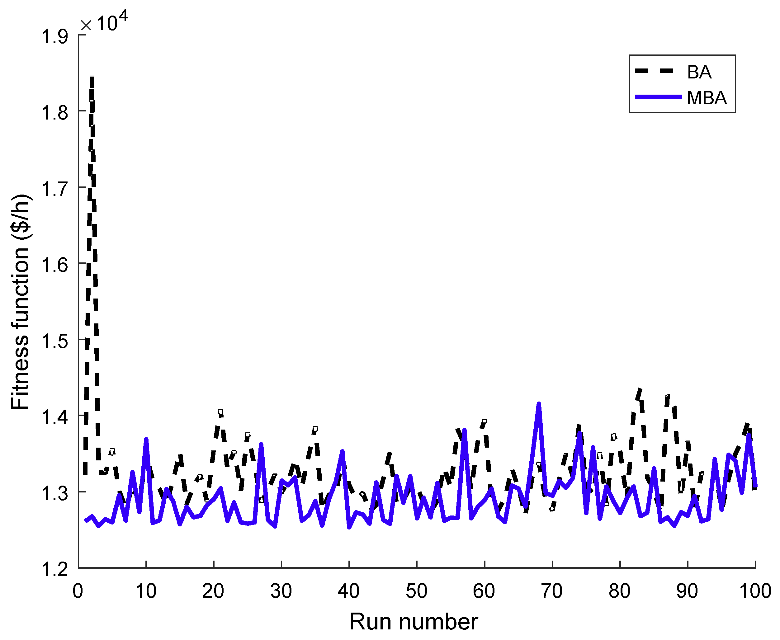Figure 4 plots the fluctuation of 100 obtained fitness function values by BA at r₀ = 0.6 and the proposed method at r₀ = 0.9. This figure shows that the proposed method has obtained higher peak than BA while the stabilization of 100 runs of the proposed method is much better than those from BA. Most of runs, MBA has yielded better optimal solutions than BA because most points of MBA are below points of BA. On the other hand, there are many solutions having approximate fitness functions with the best solution of MBA while points that are close to the best point of BA are few.

Table 4. Result comparison among methods for Case 1.

Method	Min Cost ($/h)	NP/Gmax	FEmax	CPU (S)	Processor	SCT (S)	SCT (Pu)
BCO [14]	10,317	50/100	5000	5.1563	3	6.45	64.45
RCGA [14]	10,667	100/100	10,000	6.4723	3	8.09	80.90
AIS [17]	10,355	50/100	5000	5.2956	3	6.62	66.20
EP [17]	10,390	100/100	10,000	5.3274	3	6.66	66.59
PSO [17]	10,613	100/100	10,000	5.3944	3	6.74	67.43
LCPSO [23]	10199.5458	10/2000	20,000	1.02	1.8	0.77	7.65
LCPSO-CD [23]	10279.1023	10/2000	20,000	1.02	1.8	0.77	7.65
LWPSO [23]	10194.0217	10/2000	20,000	1.03	1.8	0.77	7.73
LWPSO-CD [23]	10265.6716	10/2000	20,000	1.02	1.8	0.77	7.65
GCPSO [23]	10143.7898	10/2000	20,000	1.01	1.8	0.76	7.58
GCPSO-CD [23]	10294.2369	10/2000	20,000	1.02	1.8	0.77	7.65
GWPSO [23]	10243.0249	10/2000	20,000	1.03	1.8	0.77	7.73
GWPSO-CD [23]	10281.6835	10/2000	20,000	1.03	1.8	0.77	7.73
CSA [26]	10177.67	10/1500	30,000	1.2	1.8	0.90	9.00
GWO [25]	10111.24	-/200	-	5.26	2.3	5.04	50.41
BA	10376.4676	40/200	8000	0.154	2.4	0.15	1.54
MBA	10177.3323	20/200	4000	0.1	2.4	0.1	1

illustrates the minimum cost, execution time, and associated information with the comparison of computational time (CPU time) using MBA and other methods. Observing this table, the fuel cost comparison indicates that MBA finds a better optimal solution than most methods excluding two methods, that are GCPSO [23] and GWO [25] with slightly less costs of $33.54 and $66.09 than MBA, respectively. Despite the disadvantage, MBA is still a the strongest method since its CPU time is the fastest among the compared methods, especially 1.01 s for GCPSO [23] and 5.26 s for GWO [25] while that is only 0.1 second for MBA. Moreover, as indicated in the FE_max and SCT (s) columns, MBA used 4000 fitness evaluations and spent a runtime of 0.1 second, which are lower than all other methods like BCO [14] and AIS [17], that used 5,000 fitness evaluations and take 6.45 s and 6.62 s, respectively. When compared to GCPSO [23] and GWO [25], FE_max and SCT(s) are 20,000 and 0.76 s when using GCPSO, respectively. Whilst there was no population size reported when using GWO, it has taken a quite long time of 5.04 s to search the solution. For the SCTs (PU), MBA is much faster than other methods by 50.41, 64.45 and 80.90 times corresponding to GWO [25], BCO [14] and RCGA [14], respectively. Based on three comparisons, we conclude that the proposed method is a very efficient method for solving the CHPGED problem for a system with seven units. The optimal solution obtained for this study case is given in

Table A4. The best solution obtained by the proposed MBA method for test system 1.

Pp1(MW)	53.8546	Pp4 (MW)	211.1972	Hc1 (MWth)	43.9396
Pp2 (MW)	101.4966	Pc1 (MW)	91.4051	Hc2 (MWth)	73.9860
Pp3 (MW)	109.797	Pc2 (MW)	40.1921	Hk1 (MWth)	32.0744

in the Appendix.

4.2. Case 2

The power system with 24 generation units consisting of 13 pure power generation units, five pure heat generation units, and six cogeneration units, is considered to be the second study case. This power system supplies an electricity power demand of the electrical load demand 2350 MW and a heat load demand of 1250 MWth. The data of this system has been taken from [18] and are given in

Table A5. Characteristic of cogeneration units for case 2.

Unit	acj	bcj	ccj	kcj	lcj	mcj	Feasible regions [Pcj, Hcj]
1	2650	14.5	0.0345	4.2	0.03	0.031	[98.8,0], [81, 104.8], [215, 180], [247, 0]
2	1250	36	0.0435	0.6	0.027	0.011	[44, 0], [44, 15.9], [40, 75], [110.2, 135.6], [125.8, 32.4], [125.8, 0]
3	2650	14.5	0.0345	4.2	0.03	0.031	[98.8, 0], [81, 104.8], [215, 180], [247, 0]
4	1250	36	0.0435	0.6	0.027	0.011	[44, 0], [44, 15.9], [40, 75], [110.2, 135.6], [125.8, 32.4], [125.8, 0]
5	2650	34.5	0.1035	2.203	0.025	0.051	[20, 0], [10, 40], [45, 55], [60, 0]
6	1565	20	0.072	2.34	0.02	0.04	[35, 0], [35, 20], [90, 45], [90, 25], [105, 0]

,

Table A6. Characteristic of pure power generation units for case 2.

Unit	api	cpi	bpi	epi	fpi	$[{\mathit{P}}_{\mathit{p}\mathit{i}}^{\mathbf{min}},{\mathit{P}}_{\mathit{p}\mathit{i}}^{\mathbf{max}}]$
1	550	8.1	0.00028	300	0.035	[0, 680]
2	309	8.1	0.00056	200	0.042	[0, 360]
3	309	8.1	0.00056	200	0.042	[0, 360]
4	240	7.74	0.00324	150	0.063	[60, 180]
5	240	7.74	0.00324	150	0.063	[60, 180]
6	240	7.74	0.00324	150	0.063	[60, 180]
7	240	7.74	0.00324	150	0.063	[60, 180]
8	240	7.74	0.00324	150	0.063	[60, 180]
9	240	7.74	0.00324	150	0.063	[60, 180]
10	126	8.6	0.00284	100	0.084	[40, 120]
11	126	8.6	0.00284	100	0.084	[40, 120]
12	126	8.6	0.00284	100	0.084	[55, 120]
13	126	8.6	0.00284	100	0.084	[55, 120]

and

Table A7. Characteristic of pure heat generation unit for case 2.

Unit	ahk	bhk	chk	$[{\mathit{H}}_{\mathit{h}\mathit{k}}^{\mathbf{min}},{\mathit{H}}_{\mathit{h}\mathit{k}}^{\mathbf{max}}]$
1	950	2.0109	0.038	[0, 2695.20]
2	950	2.0109	0.038	[0, 60]
3	950	2.0109	0.038	[0, 60]
4	480	3.0651	0.052	[0, 120]
5	480	3.0651	0.052	[0, 120]

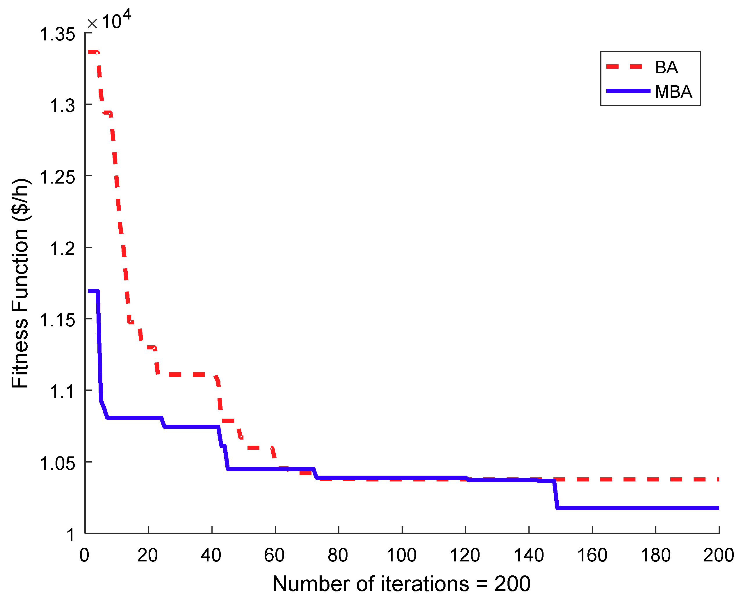
in the Appendix. The two control parameters N_B and G_max are set at 40 and 200 for BA, respectively; and set at 20 and 150 for MBA, respectively. For the study case, SR when applying BA is 74.6% poorer than that applying MBA which is 92.8%. For the minimum fuel costs, when applying BA and MBA, they are $58,198.82 and $57,851.9133, respectively. 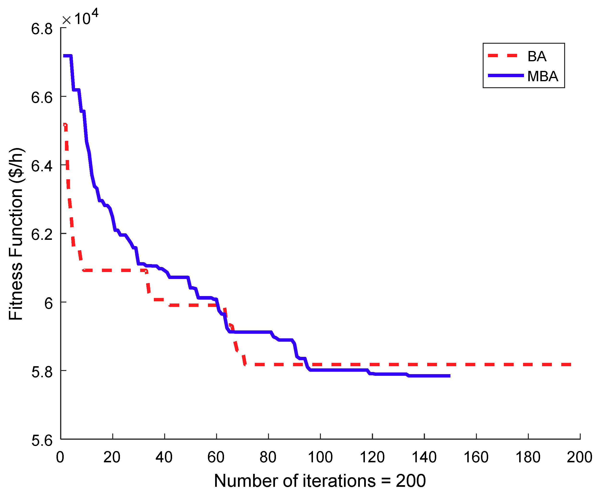The fitness function value of the best solution from the 2nd iteration onwards, when using BA and MBA, is plotted in Figure 5. Observing this figure, from the beginning to the 90th iteration, BA and MBA have found approximately good solutions and it is difficult to state which one is better than the other, however, from the 90-th iteration to the end of the search process, BA has failed to improve its search ability because the fitness function values seemed to decrease inconsiderably and it have trapped at a local optimum. Unlikely BA, MBA has still improved its solutions gradually and its fitness function values have been much lower than those of BA. This means that MBA could tackle the local optimum better than BA. 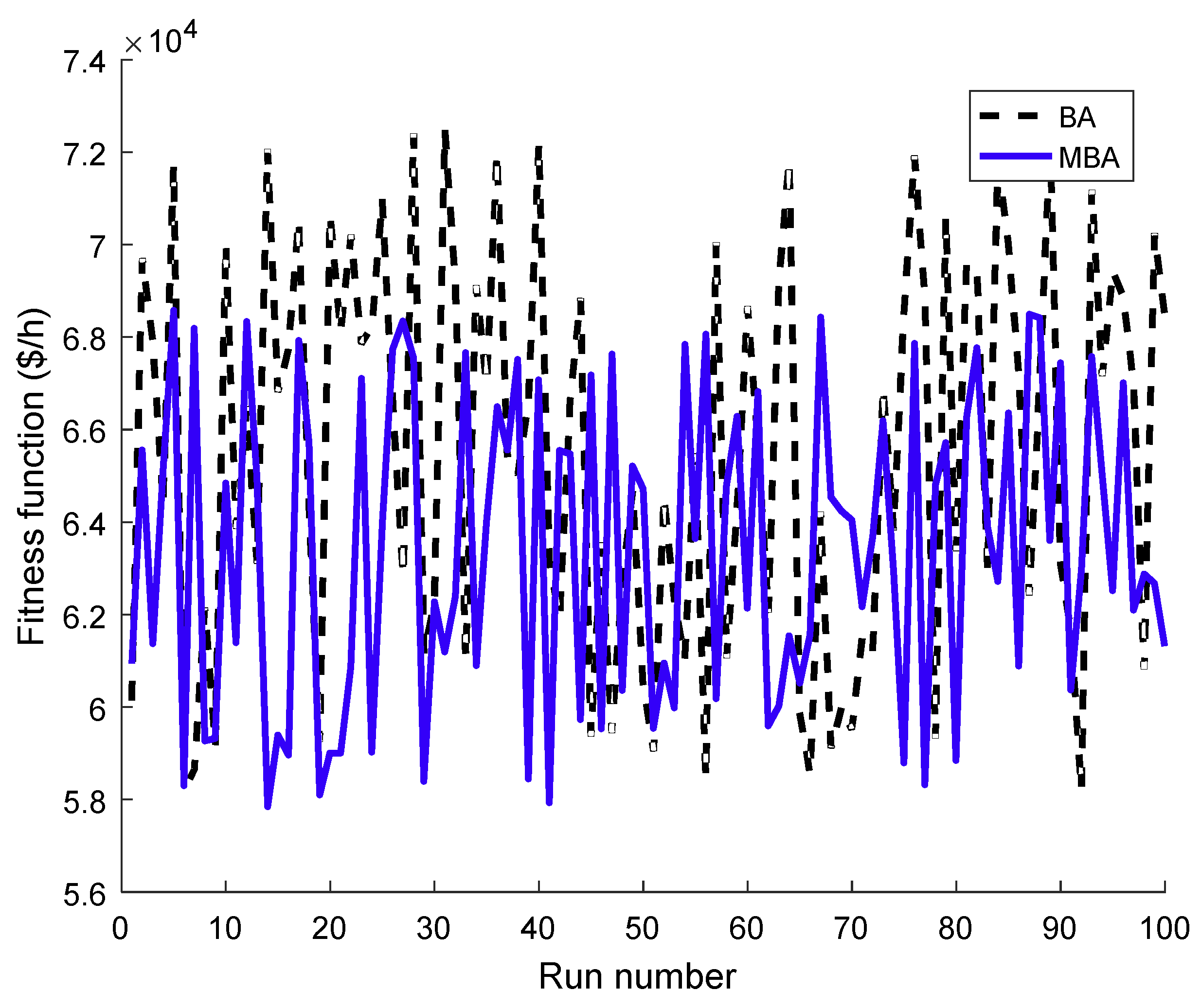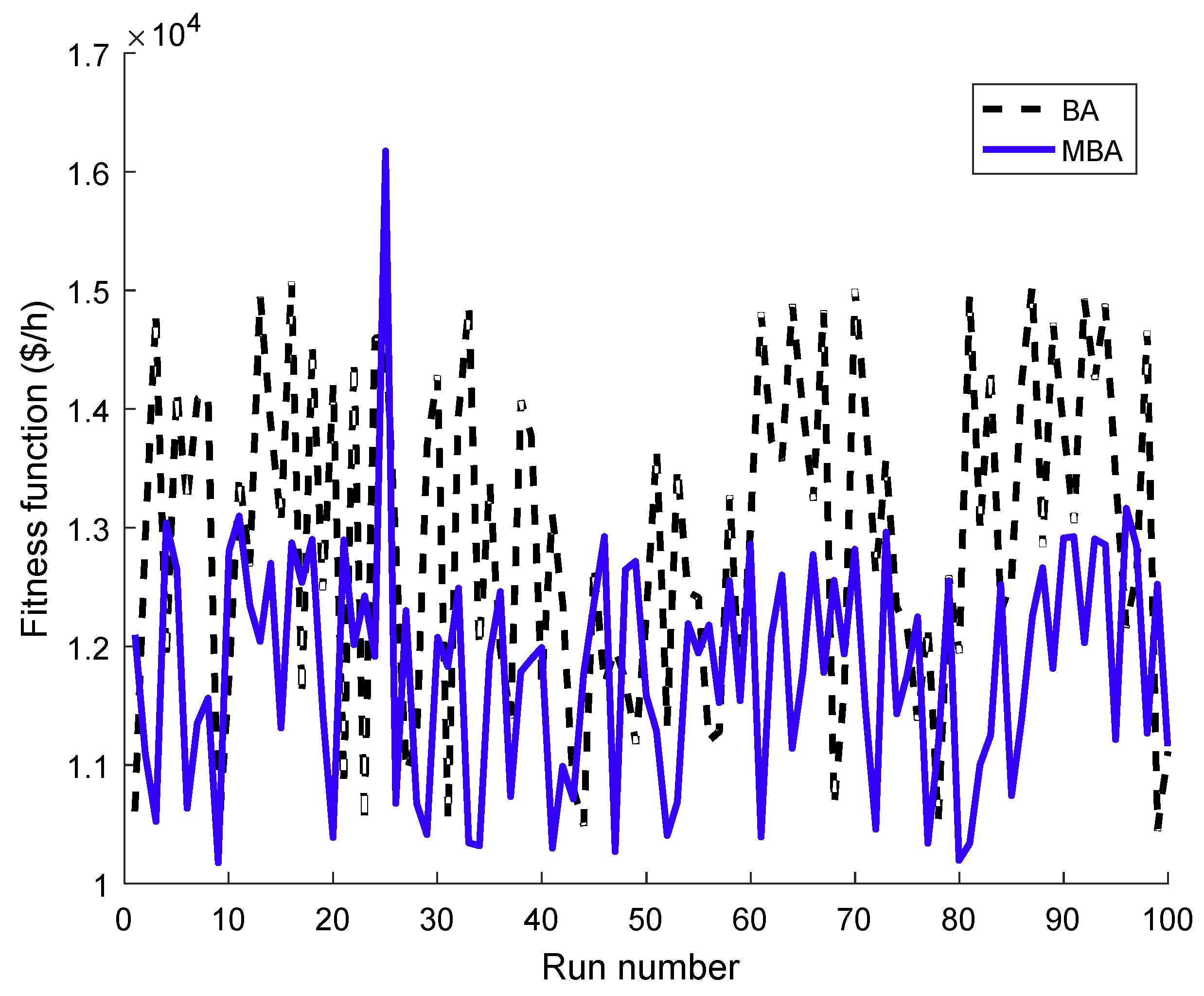Figure 6 plots the 100 fitness function values of BA and MBA. Observing this figure, MBA is superior to BA because most points of MBA are below those of BA. Besides, the differences of fitness function values of BA and MBA are too high, leading to a space above with approximately black color while the space below with approximately blue color. Other information that can be seen is that MBA can search many solutions of similar quality for the best solution.

Table 5. Result comparison for Case 2.

Method	Min. Cost ($/h)	NP	Gmax	FEmax	CPU Time (S)	Processor (Ghz)	SCT (S)	SCT (PU)	Saving Cost ($/h)
PSO [18]	59,736.26	500	2000	1,000,000	53.36	2.0	44.47	635.29	1884.3467
TVAC-PSO [18]	58,122.75	500	2000	1,000,000	52.25	2.0	43.54	622.00	270.8367
CGSO [19]	58,225.75	25	300	7500	35.54	2.5	37.02	528.86	373.8367
IGSO [19]	58,049.02	25	300	7500	35.54	2.5	37.02	528.86	197.1067
TLBO [21]	58007	50	300	15,000	5.67	2.53	5.98	85.43	155.0867
OTLBO [21]	57,856.27	50	300	15,000	5.82	2.53	6.14	87.71	4.3567
GWO [24]	57,846.84	30	45	1350	5.48	2.3	5.25	75.00	−5.0733
GSO [20]	57,843.52	100	200	20,000	5.41	3.0	6.76	96.57	−8.3933
OBGSO [22]	57,829.25	100	200	20,000	5.63	3.0	7.04	100.57	−22.6633
BA	58,198.82	40	200	8000	0.1	2.4	0.1	1.43	346.9067
MBA	57,851.91	20	150	3000	0.07	2.4	0.07	1.00	-

lists a comparison of the results yielded by many reference methods. The minimum cost yielded by MBA is $ 57,851.9133, which is less than most methods eliminating GSO [20], OBGSO [22] and GWO [24]. The comparison implies that the proposed method is ranked as the fourth best optimal solution among the compared methods. In addition, to indicate the exact amount of money that MBA can save compared to others, we have calculated the saving cost by determining the difference between the reported cost from others and that from MBA as shown in the last column of Table 5. Observing this figure, MBA obtained a higher cost than GSO [20], OBGSO [22] and GWO [24] by $5.0733, $8.3933 and $22.6633, respectively. Compared to other methods, MBA can save from $4.3567 to $1884.3467 related to OTLBO [21] and PSO [18], respectively. On the other hand, to apply fair comparisons among the different methods, the values of FE_max and SCT (in seconds and PU) have also been calculated and listed in Table 5. It is shown in this table that MBA has employed the second lowest FE_max with 3,000 fitness evaluations, which is only higher than that of GWO [24] (1350 fitness evaluations) and significantly less than 1,000,000 of PSO as well as TVAC-PSO [18]. As for the criterion of convergence speed, MBA is outstanding over all other methods, e.g., 75 times faster than GWO [24] and 635.29 times as fast as PSO [18]. In this criterion, BA is also faster than all methods except MBA with the SCT (in PU) of 1.43 (i.e., 1.43 times slower than MBA). Based on the three advantages over other methods including the best optimal solution, the second lowest FE_max and the fastest convergence speed, the proposed MBA is absolutely superior to all methods and it is a very efficient method for solving the CHPGED problem in the system with 24 units. The optimal solution obtained by the proposed MBA for case 2 is given in

Table A8. The best solution obtained by the proposed MBA method for test system 2.

Pp1 (MW)	538.5749	Pp11 (MW)	77.2659	Hc2 (MWth)	75.4862
Pp2 (MW)	299.4602	Pp12 (MW)	55.0000	Hc3 (MWth)	104.8000
Pp3 (MW)	299.4602	Pp13 (MW)	55.0000	Hc4 (MWth)	75.4862
Pp4 (MW)	109.9476	Pc1 (MW)	81.0000	Hc5 (MWth)	40.0444
Pp5 (MW)	109.9476	Pc2 (MW)	40.5637	Hc6 (MWth)	20.0131
Pp6 (MW)	109.9476	Pc3 (MW)	81.000	Hk1 (MWth)	469.3734
Pp7 (MW)	109.9476	Pc4 (MW)	40.5637	Hk2 (MWth)	59.9983
Pp8 (MW)	109.9476	Pc5 (MW)	10.1044	Hk3 (MWth)	59.9983
Pp9 (MW)	109.9476	Pc6 (MW)	35.0557	Hk4 (MWth)	120.0000
Pp10 (MW)	77.2659	Hc1 (MWth)	104.8	Hk5 (MWth)	120.000

in the Appendix.

4.3. Case 3

In order to investigate more the capability of the proposed method, in this case study, we consider a large-scale power system with 48 units, consisting of 26 pure power generation units, 10 pure heat generation units, and 12 cogeneration units. This power system supplies a 2500 MWth heat demand and a 4700 MW power demand [18]. The data of the system can be obtained by duplicating the data of System 2 in Case 2. The control parameters N_B and G_max are fixed at 60 and 200 for BA, respectively; and they are fixed at 30 and 200 for MBA, respectively. 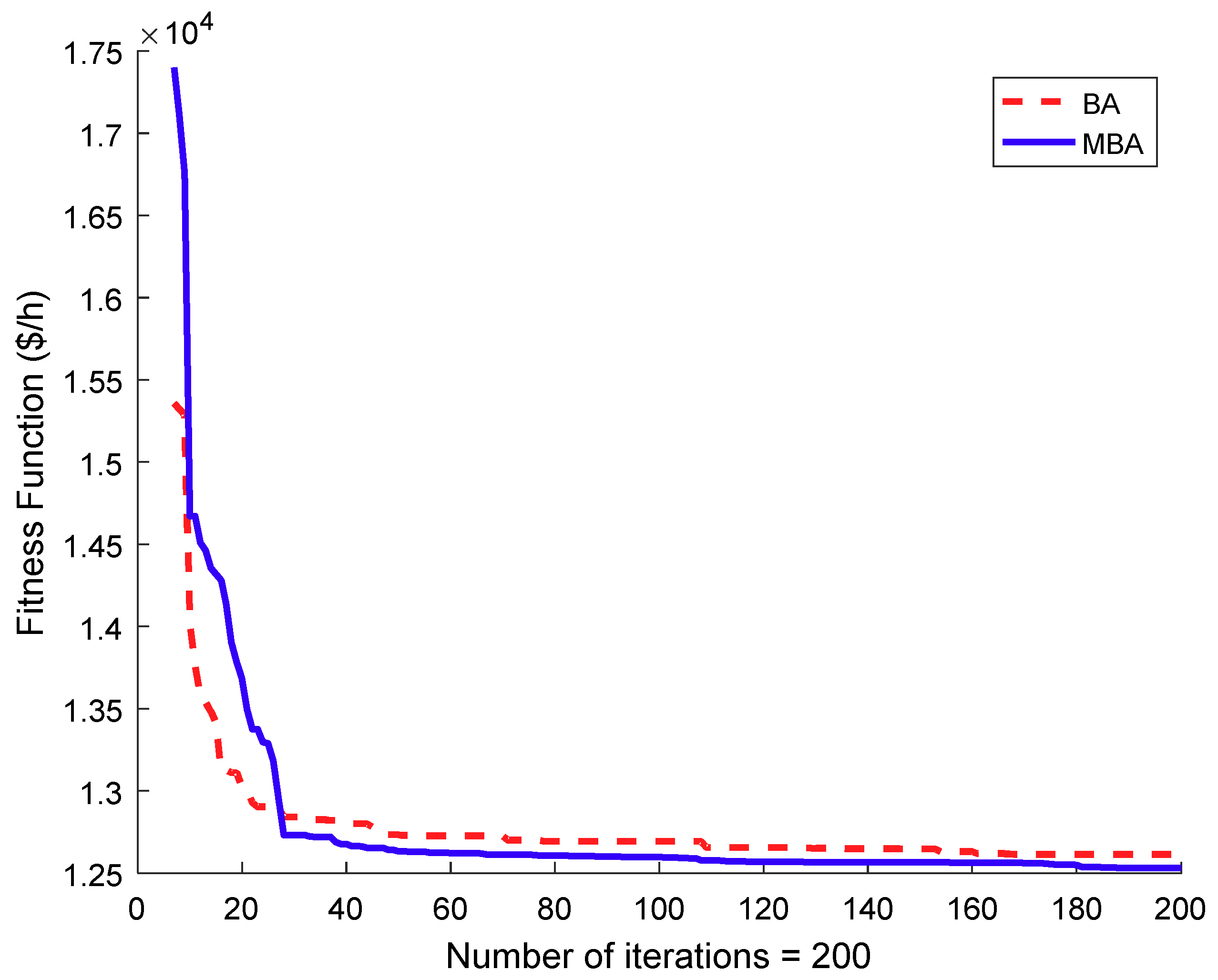Figure 7 plots the fitness function value of the best solution between the 3rd iteration and the 200th iteration obtained when applying BA and MBA, respectively. In general, the best solutions from the two methods could dramatically increase their quality during the first half of the process, afterwards they showed a slight decrease and finally reached the lowest value at the end of the search. However, as shown in Figure 7, the rate of improvement of the fitness values in MBA has been higher than that in BA during the search process, and especially during the last twenty iterations, where MBA’s fitness values have been still decreased significantly but BA’s fitness values have almost kept constant. Similar to the previous Cases 1 and 2, BA has still become trapped in a local optimum while MBA could tackle the drawback for the case. Figure 8 can confirm the superiority of MBA over BA as in Cases 1 and 2 as most points of MBA are below those from BA. However, there is a big difference in this figure compared to Figure 4 and Figure 6 in that MBA has more stable search than BA for the complicated case with 48 units and non-convex fuel cost function because the points of BA are in the the upper space while the space below belongs to the points of MBA.

Table 6. Result comparison for Case 3.

Method	Min. Cost ($/h)	NP	Gmax	FEmax	CPU	Processor (Ghz)	SCT (S)	SCT (Pu)	Saving Cost ($)
PSO [18]	119,708.8818	500	2000	1,000,000	93.32	2.0	77.8	972.5	3742.8586
TVAC-PSO [18]	117,824.896	500	2000	1,000,000	89.63	2.0	74.7	933.75	1858.8728
GSO [20]	116,457.96	200	300	60,000	9.51	3.0	11.9	148.75	491.9368
TLBO [21]	116,739.364	50	300	15,000	10.38	2.53	10.9	136.25	773.3408
OTLBO [21]	116,579.239	50	300	15,000	10.93	2.53	11.5	143.75	613.2158
OBGSO [22]	116,403.331	200	300	60,000	9.87	3.0	12.3	153.75	437.3078
LCPSO [23]	117,248.7934	20	80,000	1,600,000	72.4	1.8	54.3	678.75	1282.7702
LCPSO-CD [23]	117,164.117	20	80,000	1,600,000	69.8	1.8	52.4	655	1198.0938
LWPSO [23]	117,088.3912	20	80,000	1,600,000	71.6	1.8	53.7	671.25	1122.368
LWPSO-CD [23]	116,859.8498	20	80,000	1,600,000	73.7	1.8	55.3	691.25	893.8266
GCPSO [23]	117,374.0338	20	80,000	1,600,000	74.5	1.8	55.9	698.75	1408.0106
GCPSO-CD [23]	117,537.475	20	80,000	1,600,000	68.7	1.8	51.5	643.75	1571.4518
GWPSO [23]	116,572.7024	20	80,000	1,600,000	65.7	1.8	49.3	616.25	606.6792
GWPSO-CD [23]	116,768.1356	20	80,000	1,600,000	73.4	1.8	55.1	688.75	802.1124
CSA [26]	116,843.3	50	30,000	1,500,000	62.7	1.8	47	587.5	877.2768
BA	117,627.2256	60	200	12,000	0.11	2.4	0.1	1.25	1661.2024
MBA	115,966.0232	30	200	6000	0.08	2.4	0.08	1	-

shows the results in terms of minimum cost, computational time, FE_max, and SCT (in second and PU) of BA, MBA and other methods. In addition, the saving costs have also been included in the table for further comparisons similar to the two previous cases. As seen from this table, the modifications on MBA are successful for searching for an optimal solution since MBA can obtain better minimum fuel cost, lower FE_max, and faster SCT compared to its original BA. In fact, these values from MBA are $115966.0232, 6000 fitness evaluations, and 0.08 s, respectively; which are much lower than $117627.2256, 12,000 fitness evaluations and 0.1 s from BA, respectively. A further investigation of the efficiency of MBA can be executed by focusing on the saving cost and the SCT in PU. Clearly, MBA is much more effective and robust than all methods because it can save huge amounts of money and converges to an optimum significantly faster. For instance, it can save more money and is faster than TVAC-PSO [18] by $1858.8728 and 972.5 times, GSO [20] by $491.9368 and 148.75 times, TLBO [21] by $773.3408 and 136.25 times, OBGSO [22] by $ 437.3078 and 153.75 times, GWPSO-CD [23] by $802.1124 and 688.75 times, and CSA [26] by $877.2768 and 587.5 times. These compared methods are either well-known original algorithms or improved variants of original algorithms, which have been famous and superior to others in previously published articles. From the three advantages of the MBA over all methods such as the lowest minimum cost, lowest maximum number of fitness evaluations and fastest convergence speed, it can be concluded that MBA is the most efficient method for solving the system up to 48 units considering valve effects on pure power generation units. The optimal solution obtained by the proposed MBA for the case is given in

Table A9. The best solution obtained by the proposed MBA method for test case 3.

Pp1 (MW)	536.3301	Pp21 (MW)	109.1864	Hc3 (MWth)	75.0927
Pp2 (MW)	298.7655	Pp22 (MW)	109.1864	Hc4 (MWth)	75.0927
Pp3 (MW)	298.7655	Pp23 (MW)	40.0095	Hc5 (MWth)	40.2060
Pp4 (MW)	109.1864	Pp24 (MW)	40.0095	Hc6 (MWth)	20.1698
Pp5 (MW)	109.1864	Pp25 (MW)	91.98	Hc7 (MWth)	105.1408
Pp6 (MW)	109.1864	Pp26 (MW)	91.9800	Hc8 (MWth)	105.1408
Pp7 (MW)	109.1864	Pc1 (MW)	81.6105	Hc9 (MWth)	75.0927
Pp8 (MW)	109.1864	Pc2 (MW)	81.6105	Hc10 (MWth)	75.0927
Pp9 (MW)	109.1864	Pc3 (MW)	40.1085	Hc11 (MWth)	40.2060
Pp10 (MW)	40.0095	Pc4 (MW)	40.1085	Hc12 (MWth)	20.1698
Pp11 (MW)	40.0095	Pc5 (MW)	10.4829	Hk1 (MWth)	465.8057
Pp12 (MW)	91.98	Pc6 (MW)	35.3783	Hk2 (MWth)	60.0000
Pp13 (MW)	91.98	Pc7 (MW)	81.6105	Hk3 (MWth)	60.0000
Pp14 (MW)	551.8145	Pc8 (MW)	81.6105	Hk4 (MWth)	120.0000
Pp15 (MW)	298.7655	Pc9 (MW)	40.1085	Hk5 (MWth)	120.0000
Pp16 (MW)	298.7655	Pc10 (MW)	40.1085	Hk6 (MWth)	472.5088
Pp17 (MW)	109.1864	Pc11 (MW)	10.4829	Hk7 (MWth)	60.0000
Pp18 (MW)	109.1864	Pc12 (MW)	35.3783	Hk8 (MWth)	60.0000
Pp19 (MW)	109.1864	Hc1 (MWth)	105.1408	Hk9 (MWth)	120.0000
Pp20 (MW)	109.1864	Hc2 (MWth)	105.1408	Hk10 (MWth)	120.0000

in Appendix A.

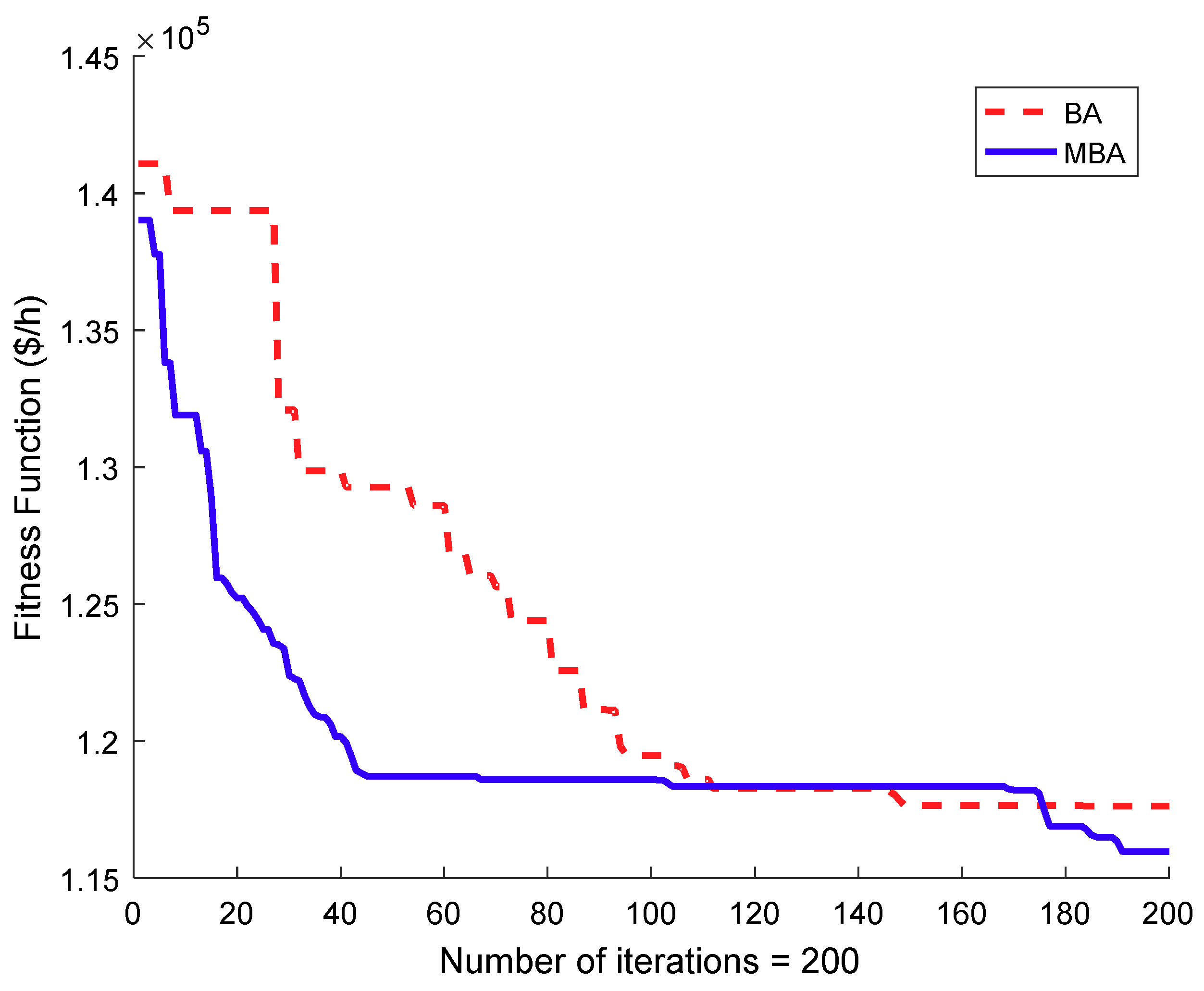
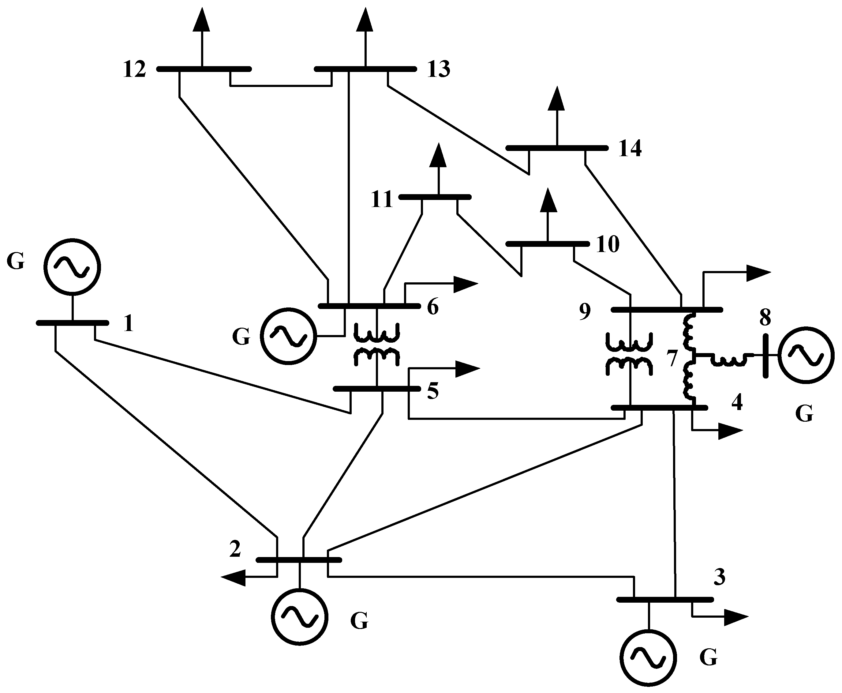
4.4. Case 4

In order to evaluate the MBA capability of dealing with the ccomplicated constraints of the CHPGED problem, we have tested both MBA and BA in study Case 4 with the use of an IEEE 14-bus system. The original IEEE 14-bus system shown in Figure 9 covers five generators located at five different buses 1, 2, 3, 6 and 8, 15 load buses, 20 transmission branches, and three transformers and one compensator. For application of the combined heat and power generation units, we have replaced the pure power generation units at bus 2 and bus 3 with two different cogeneration units, which have been taken from [18]. In addition, one pure heat generation unit taken from [18] has also been installed for supplying heat to load in addition to the heat from the two cogeneration units. The power demand of 15 loads is 259 MW while the heat demand of load is supposed to be 400 MWth. The whole data of the IEEE 14-bus system can be obtained by referring to [40] while the entire data of three pure power generation units, two cogeneration units and one pure heat generation unit are given in

Table A10. Characteristic of cogeneration units for case 4.

Location	acj	bcj	ccj	lcj	kcj	mcj	Feasible regions [Pcj, Hcj]	$[{\mathit{Q}}_{\mathit{c}\mathit{j}}^{\mathbf{min}},{\mathit{Q}}_{\mathit{c}\mathit{j}}^{\mathbf{max}}]$
Bus 2	2650	34.5	0.1035	0.025	2.203	0.051	[20, 0], [10, 40],[45, 55], [60, 0]	[−40, 50]
Bus 3	1565	20	0.072	0.02	2.34	0.04	[35, 0], [35, 20], [90, 45], [90, 25], [105, 0]	[0, 40]

,

Table A11. Characteristic of pure power generation units for case 4.

Location	api	cpi	bpi	cpi	epi	fpi	$[{\mathit{P}}_{\mathit{p}\mathit{i}}^{\mathbf{min}},{\mathit{P}}_{\mathit{p}\mathit{i}}^{\mathbf{max}}]$	$[{\mathit{Q}}_{\mathit{p}\mathit{i}}^{\mathbf{min}},{\mathit{Q}}_{\mathit{p}\mathit{i}}^{\mathbf{max}}]$
Bus 1	150	0.00016	2.0	0.00016	50	0.0630	[50, 200]	[−40, 100]
Bus 6	0	0.00834	3.25	0.00834	0	0	[10, 35]	[−6, 24]
Bus 8	0	0.025	3	0.025	0	0	[10, 30]	[−6, 24]

and

Table A12. Characteristic of pure heat generation unit for case 4.

chk	bhk	ahk	$[{\mathit{H}}_{\mathit{h}\mathit{k}}^{\mathbf{min}},{\mathit{H}}_{\mathit{h}\mathit{k}}^{\mathbf{max}}]$
0.038	2.0109	950	[0, 400]

of Appendix A.

For implementing BA and MBA, we have set N_B and G_max to 20 and 150. As a result, BA could not deal with the constraints successfully whilst MBA could achieve a success rate of lower than 50% but the optimal solutions were of low quality. Thus, we have increased the two parameters to 20 and 200 for MBA but 40 and 200 for BA.

Table 7. Results obtained by BA and MBA for IEEE 14-bus system.

r0	Min. Cost ($/h)		Average Cost ($/h)		Successful Rate (%)		Saving Cost ($/h)
	BA	MBA	BA	MBA	BA	MBA
0.1	12,954.38546	12,600.5759	13,941.01584	13,048.5264	67%	88%	353.80956
0.2	12,730.4359	12,597.6011	13,163.772	12,987.8871	69%	90%	132.8348
0.3	12,700.5991	12,568.8029	13,344.9665	12,892.5259	71%	92%	131.7962
0.4	12,928.5284	12,578.4712	13,914.9948	12,882.534	73%	93%	350.0572
0.5	12,679.384	12,544.0718	13,218.1625	12,970.4853	75%	93%	135.3122
0.6	12,669.95783	12,563.0969	13,196.25723	12,974.4669	74%	95%	106.86093
0.7	12,668.3388	12,552.5954	13,193.6942	12,984.5393	77%	94%	115.7434
0.8	12,632.0112	12,532.4616	13,169.9174	12,827.6351	767%	95%	99.5496
0.9	12,614.0837	12,532.4717	13,001.5593	12,785.6208	76%	95%	81.612

shows minimum cost, average cost and success rate obtained by BA and MBA for 100 successful runs. As we may observe, the minimum values of BA and MBA can show that MBA could find better optimal solutions than BA corresponding to each value of r₀. The savings cost also indicates that MBA could improve the results from $81.612 to $353.80956. The best minimum of BA is $12,614.0837 while that of MBA is $12,532.4616. Clearly, MBA could improve results over BA by 0.65%. However, the result can be improved more significantly if we decrease N_B of BA to 20 or we increase N_B of MBA to 40. Although MBA has used a smaller population size it always get a higher success rate than BA. The highest SR of MBA is approximately 95% at r₀ = 0.6, 0.8 and 0.9, but BA only gets 77% at r₀ = 0.7. The search process of the best run of BA at r₀ = 0.9 and MBA at r₀ = 0.8 are depicted in Figure 10. 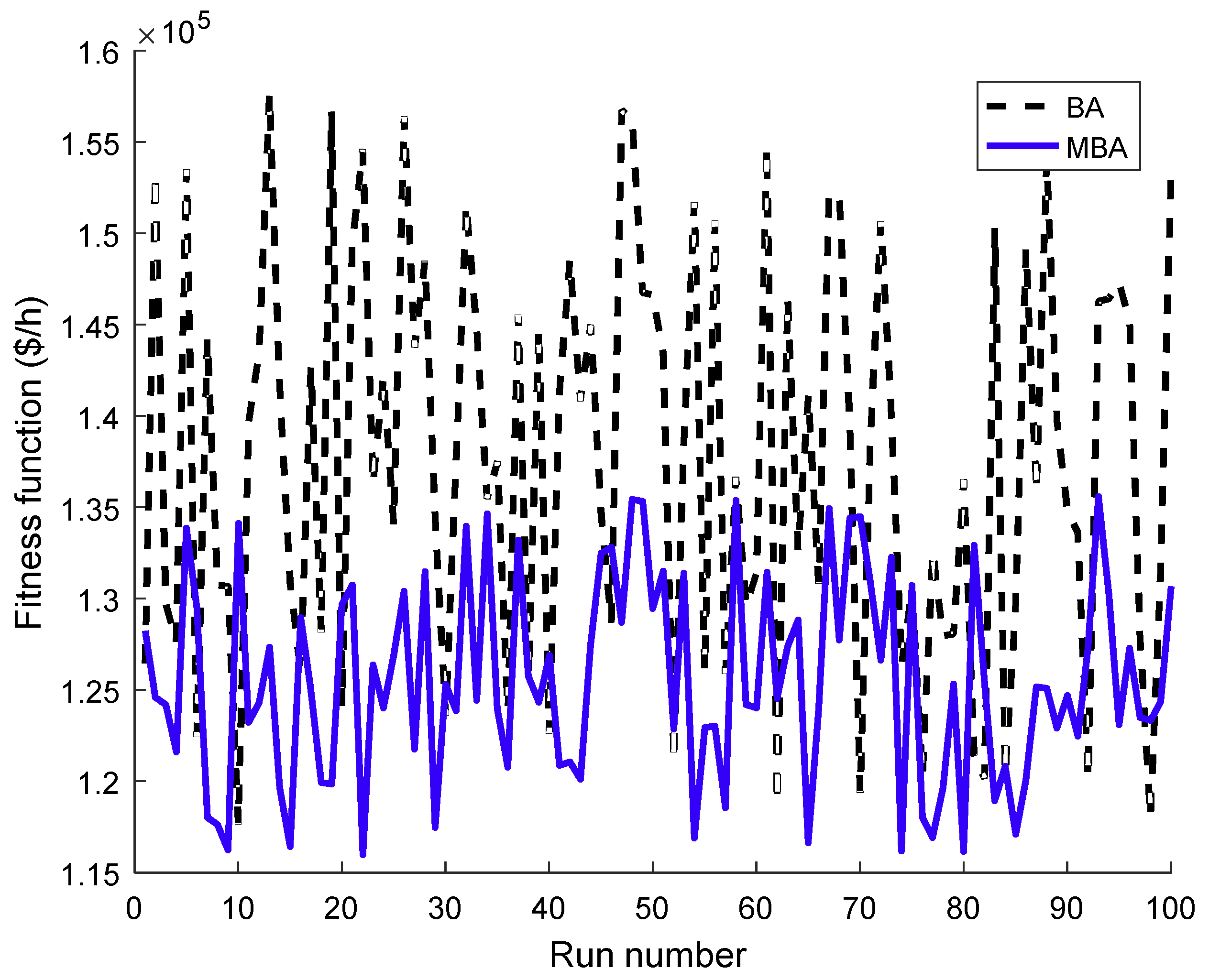Besides, the best cost of 100 successful runs of BA at r₀ = 0.9 and MBA at r₀ = 0.8 are shown in Figure 11. Figure 10 indicates that MBA could find better solutions than BA after the 23rd iteration, and the solution of MBA at iteration 120 had a lower cost than that of BA at the final iteration. It is clearly visible that MBA was faster than BA. On the other hand, MBA also shows its better stability since most runs of MBA had a lower cost than those of BA as shown in Figure 11. Thus, we can conclude that MBA can deal with the complicated constraints of CHPGED problems considering a transmission power network and its performance is significantly improved compared to BA. The optimal solution of MBA can be obtained by referring to

Table A13. Optimal solution obtained by BA and MBA for case 4.

Variables	BA	MBA
Hc1 MWth)	40.0045	39.9652
Hc2 MWth)	29.4753	26.3730
Hk1 MWth)	330.5203	333.6618
Pp1 (MW)	153.9262	143.8280
Pc1 (MW)	10.0000	10.0147
Pc2 (MW)	56.0605	49.0263
Pp2 (MW)	27.6515	34.4462
Pp3 (MW)	17.0759	27.1244
Vg1 (pu)	1.0511	1.0872
Vg2 (pu)	1.0242	1.0421
Vg3 (pu)	0.9973	1.0169
Vg6 (pu)	0.9980	1.0997
Vg8 (pu)	0.9812	1.0664
T8 (pu)	0.9743	0.9967
T9 (pu)	0.9670	0.9140
T10 (pu)	1.0080	0.9211
Qc9 MVAr)	11.1043	4.6189

in Appendix A.

5. Conclusions

This paper has proposed a novel modified Bat algorithm (MBA) developed based on the conventional bat algorithm (BA) with the purpose of finding high quality solutions for CHPGED problems. Challenges to MBA arise from non-convex objective functions and the complicated constraints of CHPGED problems. Complex non-convex objective functions are caused by the consideration of valve point loading effects on pure power generation unit while the complex constraints are from the feasible working zone of cogeneration units and of all components in transmission power network of IEEE 14-bus system. This proposed method has been constructed by performing three modifications. The first is the adaptive frequency adjustment, the second is the optimal range of new velocities, and the third is the retained condition of a good solution. These improvements have been implemented for overcoming the shortcomings of BA. As a result, the proposed method has been more effective than BA for applications to four different CHPGED problem systems in terms of higher quality solution, higher success rate, faster search speed and more stable search ability. The comparisons with other existing methods have shown that the proposed method had the third best solution, the lowest fitness evaluations and the fastest convergence speed for the Case 1 with seven generation units, but the best method regarding its optimal solutions for the Cases 2 and 3, which were systems up to 24 and 48 generation units, respectively. MBA has continued to show its potential search by dealing with IEEE 14 bus system and obtaining outstanding cost as well as success rate as compared to BA. Consequently, we can reach the conclusion that the proposed method is a very effective method for solving combined heat and power systems with different challenges from pure generation units, cogeneration units and transmission power networks.