A Graph Theoretic Approach to Optimal Firefighting in Oil Terminals

Abstract

Effective firefighting of major fires in fuel storage plants can effectively prevent or delay fire spread (domino effect) and eventually extinguish the fire. If the number of firefighting crew and equipment is sufficient, firefighting will include the suppression of all the burning units and cooling of all the exposed units. However, when available resources are not adequate, fire brigades would need to optimally allocate their resources by answering the question “which burning units to suppress first and which exposed units to cool first?” until more resources become available from nearby industrial plants or residential communities. The present study is an attempt to answer the foregoing question by developing a graph theoretic methodology. It has been demonstrated that suppression and cooling of units with the highest out-closeness index will result in an optimum firefighting strategy. A comparison between the outcomes of the graph theoretic approach and an approach based on influence diagram has shown the efficiency of the graph approach.

1. Introduction

Small fire incidents are a common characteristic of industrial plants containing or processing combustible and flammable substances. Major fires, despite their low-probability, however, are among the most feared types of industrial accidents due to their catastrophic consequences in terms of loss of lives and assets and also a multitude of costly resources needed to control and extinguish them. Examples of major fires include series of fires—known as fire domino effect—at oil storage terminals in the UK in 2005 [1], Puerto Rico in 2009 [2], and in Brazil in 2015 [3], as well as a massive single tank fire in Singapore in 2018 [4].

Due to the importance of major fires and particularly fire domino effects, many works have been devoted to their modelling and risk assessment [5,6,7,8,9,10,11,12,13]. Engineered fire protection systems such as sprinkler systems are effective in tackling small fires and reducing the probability of small fires escalating to fire domino effects [14], but have reportedly proven ineffective in the event of major fires and already-initiated fire domino effects; this has mainly been due to damage, malfunction, or low performance of engineered fire protection systems when exposed to severe heat of fires [15,16,17,18].

Considering the inefficiency of engineered fire protection systems in case of major fires, the intervention of fire brigades to tackle the fires becomes indispensable. Nevertheless, the works devoted to the key role of firefighting in controlling and delaying fire spread have been very few [19,20]. Although available industrial fire protection codes and standards such as NFPA 11 [21], CCPS [22], and API RP-2001 [23] can be used to set baseline firefighting strategies in oil and gas facilities, they do not take into account the facility layout and limited firefighting resources, among other parameters [16,19].

The main goal of firefighting is to extinguish fires before they become large and trigger domino effects. In this regard, firefighters can adopt different strategies, which could be: (i) defensive, where the units exposed to the heat of burning units are cooled using water, (ii) offensive, where attempts are made to suppress burning units, or (iii) mixed, as a combination of the previous two strategies, which is the case in most industrial fire events [19].

If the firefighting resources (personnel, apparatus, etc.) are adequate, a firefighting strategy will include the suppression of all the burning units and the cooling of all the exposed units. However, the main challenge arises when the number of units in danger—both on fire and exposed to fire—exceeds the available firefighting resources, demanding for optimal firefighting strategies to help firefighters answer “which burning units to suppress first and which exposed units to cool first?” in anticipation of more resources becoming available, for instance, from neighboring plants or communities. Considering the two main components of firefighting strategies, the suppression of a burning unit would reduce the emitted heat radiation until the fire is completely extinguished while the cooling of an exposed unit would reduce the amount of heat radiation the unit receives and thus prevents from the spread of the fire to the unit.

The present study is thus aimed at developing a decision support methodology using graph theory for identifying optimal firefighting strategies in the case of insufficient firefighting resources. In this study, we define an optimal firefighting strategy as one which minimizes the likelihood of cascading effects in a spatial network. The application of the methodology is demonstrated via an oil storage plant. Section 2 recaps the basics of graph theory and influence diagram; in Section 3, the methodology is developed, and its application is illustrated in Section 4. The work is concluded in Section 5.

2. Materials

2.1. Graph Theory

A mathematical graph $G=\left(V,E\right)$ is a set of nodes (V) and arcs (E). Depending on whether the arcs are directed or undirected, the graph is called directed or undirected, respectively. In a directed graph, a walk from node $v_i$ to $v_j$ is a sequence of connected nodes from the former to the latter where each intermediate node can be traversed several times. A path, however, is a walk in which each intermediate node can be traversed once at most. Accordingly, the geodesic distance between $v_i$ and $v_j$, denoted as $d_{ij}$ is defined as the length of the shortest path from $v_i$ to $v_j$. In a directed graph, the distance from $v_i$ to $v_j$ is simply the number of arcs constituting the shortest path from $v_i$ to $v_j$; if there is no path between $v_i$ and $v_j$, then $d_{ij}=\infty$.

Based on the concept of geodesic distance, a number of graph metrics can be used to describe the characteristics of the nodes, the arcs, and the graph itself. Among such metrics, closeness centrality scores are very popular in modeling and defining the characteristics of spatial networks and grids [24,25,26]. The closeness of a node $v_i$ can be defined in two ways: the out-closeness of the node, $C_{out}\left(v_i\right)$, as the number of steps needed to reach from the node to every other node of the graph, and the in-closeness, $C_{in}\left(v_i\right)$, as the number of steps needed to access $v_i$ from every other node of the graph.

$$C_{out}\left(v_i\right)=\frac{1}{{{\displaystyle \sum }}_j{d}_{ij}}$$

(1)

$$C_{in}\left(v_i\right)=\frac{1}{{{\displaystyle \sum }}_j{d}_{ji}}$$

(2)

Based on the nodes centrality scores, the graph’s centrality scores can be defined. For instance, the graph’s average out-closeness, which is analogous to the graph’s average efficiency [27] can be defined as:

$$C_{out}\left(G\right)=\frac{1}{N}{{\displaystyle \sum }}_{i=1}^N{C}_{out}\left(v_i\right)$$

(3)

Graph metrics have widely been used to describe and optimize the properties of grid infrastructures and spatial networks such as water distribution networks [28,29], oil storage plants [13], and transportation networks [30].

2.2. Bayesian Network and Influence Diagram

Bayesian network (BN) is a directed graph to represent conditional dependencies among a set of random variables by means of chance nodes and arcs [31,32]. Chance nodes with arcs directed from them are called parent nodes while the ones with arcs directed into them are called child nodes. The nodes with no parents are also called root nodes, whereas the nodes with no children are known as leaf nodes.

Satisfying the Markov condition in BNs, a node is independent of its non-descendant nodes given its parent nodes. As a result, a BN factorizes the joint probability distribution of its nodes as the product of the conditional probability distributions of the variables given their immediate parents (Equation (4)). For the nodes with no parents, i.e., the root nodes, such conditional probabilities are simply replaced by marginal probabilities.

$$P\left(X_1,X_2,\dots ,X_n\right)={\displaystyle \prod }_{i=1}^{n}P\left(X_i|pa\left(X_i\right)\right)$$

(4)

where $pa\left(X_i\right)$ is the parent(s) of node $X_i$.

A BN can be extended to an influence diagram by adding decision nodes and utility nodes. Each decision node consists of a finite set of decision policies. A decision node should be assigned as the parent of chance nodes whose probability distributions depend on the decision policies. Likewise, the decision node should be the child of chance nodes whose states have to be known to the decision maker before making that specific decision. The utility node U contains utility values (positive or negative) to reflect the preferences of the decision maker regarding the outcome of each decision policy. Among the decision policies $d_i$ (i = 1, ..., m), one with the highest expected utility (EU) is then selected as the optimal decision $d^{*}$:

$$\begin{array}{c}{d}^{*}=arg maxEU\left(d_i\right)\\ d_i\end{array}\mathrm{for}i=1,\dots ,m$$

(5)

3. Methodology

3.1. An Example

Figure 1a depicts the schematics of an oil terminal which consists of six identical gasoline storage tanks. Considering tank fires as the most likely accident scenario, for illustrative purposes, the hypothetical heat radiation intensities emitted from and received by the tanks are presented as a weighted adjacency matrix in Figure 1b, where Qij is the amount of heat tank Tj receives from a tank fire at tank Ti (kW/m²). Since all the tanks are atmospheric, the minimum heat radiation to spread the fire from a burning tank to a neighboring tank can be considered as 15 kW/m² [33]. It should be noted that having the dimension of the tanks, the separation distances between them, the weather conditions, the type and amount of flammable contents, etc., consequences assessment techniques and software such as ALOHA [34] can be used to calculate accurate amounts of heat radiation. Based on the adjacency matrix, the potential fire spread paths in the terminal can be presented as a directed graph in Figure 1c.

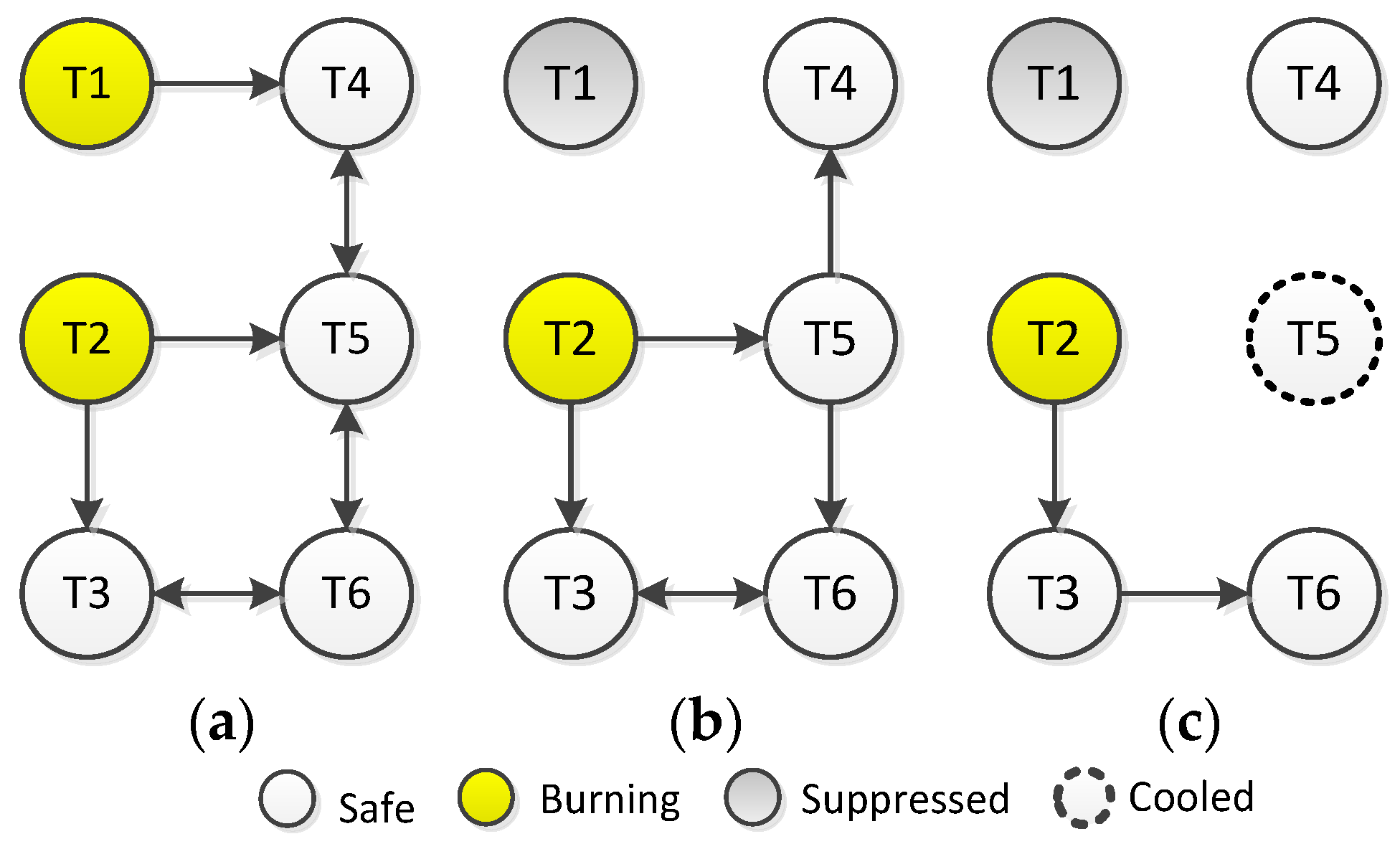
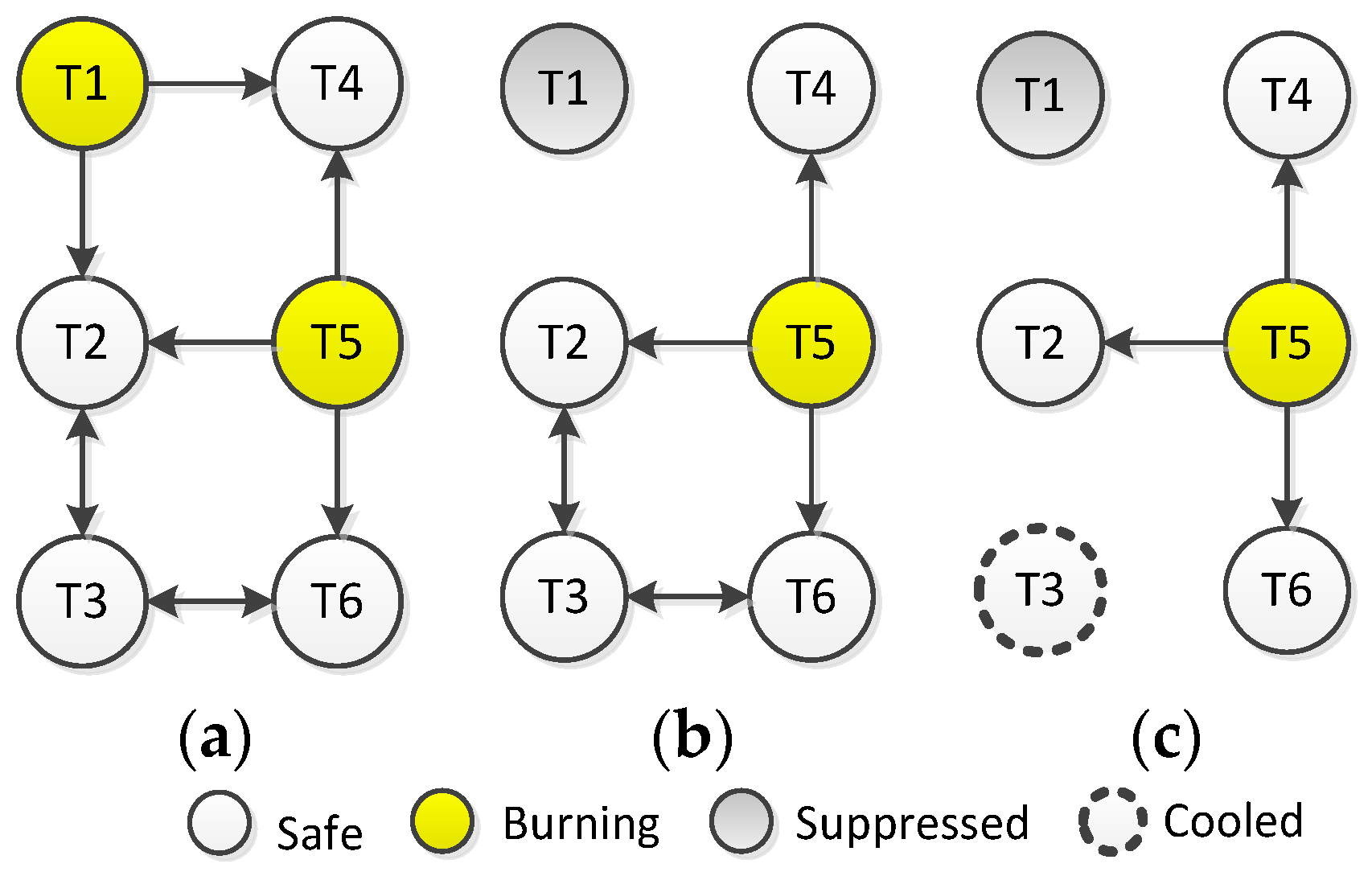
In order to identify optimal firefighting strategies under insufficient resources, we introduce some constraints to the amount and type of the available firefighting resources:

• Due to the limited amount of equipment, the fire brigade would not be able to work on more than two storage tanks at a time, and
• Out of these two storage tanks, due to limited types of equipment, one should be a burning tank and the other an exposed tank. In other words, the firefighters can only afford to suppress a burning tank and to cool another exposed tank simultaneously.
• The aim of the fire brigade would be to prevent/delay the fire spread so that the still-safe storage tanks could be saved. In other words, the suppression of a burning tank, for instance, is performed with the aim of saving the neighboring tanks rather than saving the burning tank itself.

Further, when a storage tank has been exposed to an adjacent burning tank for a while unbeknown to the firefighters, the cooling of the exposed tank would be a more conservative strategy than the suppression of the burning tank [19]; however, in the case of crude oil storage tanks, the suppression of burning tanks should be given priority over the cooling of exposed tanks, due to the imminent risk of boil-over [35].

3.2. Optimal Firefighting Using Graph Theory

Since the identification of firefighting strategies would be based on the observations made by or reported to the firefighters, three fire spread scenarios are considered:

• Scenario 1: fire starts at T1 and spreads to T2;
• Scenario 2: fire starts at T1 and spreads to T2 and T4;
• Scenario 3: two simultaneous fires start at T1 and T5.

Khakzad and Reniers [13] demonstrated that modeling cascading effects in spatial networks as a directed graph, the nodes with a higher out-closeness score (Equation (1)) would result in more extensive failures if selected as the initiating node. Similarly, they illustrated that among spatial networks of different layout but identical number of nodes, the ones with a higher average out-closeness scores (Equation (3)) are more vulnerable to the cascading failures.

3.2.1. Scenario 1: Fire Starts at T1 and Escalates to T2

In the case of fires at T1 and T2, the graph in Figure 1c should be customized to present feasible fire spread paths among the storage tanks. To this end, Figure 2a shows the customized fire spread graph where the storage tanks on fire, T1 and T2, would no longer impact one another, and the double-headed arrows between T1 and T4, T2 and T5, and T2 and T3 have been changed to single-headed arrows directed from the burning tanks to the exposed tanks. Modeling the graph of Figure 2a in igraph package [36], the out-closeness scores of the storage tanks as well as the average out-closeness score of the terminal have been calculated and listed in

Table 1. Tanks’ and terminal’s out-closeness scores for the graphs in Figure 2 and Figure 3.

	Out-Closeness Scores
	Fire Initiation	Optimal Firefighting		Non-Optimal Firefighting
Tank	Figure 2a and Figure 3a	Figure 2b	Figure 2c	Figure 3b	Figure 3c
T1	0.31	0.31	0.17	0.17	0.17
T2	0.42	0.17	0.17	0.42	0.24
T3	0.28	0.17	0.17	0.20	0.20
T4	0.28	0.28	0.17	0.17	0.17
T5	0.31	0.23	0.17	0.31	0.17
T6	0.31	0.20	0.17	0.20	0.17
Terminal	0.48	0.24	0.00	0.24	0.12

(the 2nd column).

As can be seen from Table 1, between the burning tanks in Figure 2a, the out-closeness of T2 (0.42) is larger than T1 (0.313), implying that T2 would contribute more to the spread of fire through the plant, and thus should be given priority over T1 in being suppressed. Figure 2b shows possible fire escalation patterns in the case T2 is suppressed, and thus there would no longer be any arrows from it to T1, T3, and T5. Recalculating the out-closeness scores of the nodes in Figure 2b (3rd column of Table 1), T4 has the largest out-closeness score among the exposed tanks; thus, it is given priority over the other tanks in being cooled. Figure 2c depicts the graph where T1 is still burning, T2 has been suppressed, and T4 is being cooled. Since T4 is cooled, it would no longer be impacted by T1, which is still burning, and thus the arrow from T1 to T4 should be eliminated. Likewise, since T4 would not get damaged and involved in the fire chain, there is no way that T5 could be damaged and catch fire. This is why the arrow from T4 to T5 should be eliminated, and similarly the arrows from T5 to T6 and T3. As can be noted, the graph’s average out-closeness score decreases from 0.48 in Figure 2a to 0.00 in Figure 2c (2nd and 4th columns in Table 1).

To demonstrate that the suppression of T2 and the cooling of T4 would be the optimal firefighting strategy in Scenario 1, where Figure 3a show the original fire scenario, and Figure 3b depicts a strategy in which T1 is suppressed instead of T2. Given that T1 is suppressed, consider a non-optimal strategy in Figure 4, the out-closeness scores of the tanks are calculated as in Table 1 (the 5th column), indicating T5 with the largest out-closeness score among the exposed tanks and thus the candidate for cooling.

Figure 3c depicts the graph where T1 is extinguished, T2 is still on fire, and T5 is cooled. Following this non-optimal strategy, the graph’s average out-closeness decreases from 0.48 in Figure 3a to 0.12 in Figure 3c (2nd and 6th columns in Table 1). As can be seen, adopting the former firefighting strategy (Figure 2c) would result in a lower average out-closeness score for the graph than the latter firefighting strategy (Figure 3c), and thus a weaker cascading effect (lower likelihood of fire spread) can be expected [13]. For the sake of clarity, the out-closeness scores of the critical units as well as the average out-closeness score of the plant are depicted with bold numbers in Table 1.

3.2.2. Scenario 2: Fire Starts at T1 and Spreads to T2 and T4

In this scenario, when firefighters arrive at the scene, the fire has already propagated from T1 to T2 and T4 (Figure 4a). Since T2 has the largest out-closeness score among T1 and T4 (2nd column in

Table 2. Tanks’ and terminal’s out-closeness scores for the graphs in Figure 4 and Figure 5.

	Out-Closeness Scores
	Fire Initiation	Optimal Firefighting		Non-Optimal Firefighting
Tank	Figure 4a and Figure 5a	Figure 4b	Figure 4c	Figure 5b	Figure 5c
T1	0.17	0.17	0.17	0.17	0.17
T2	0.31	0.17	0.17	0.31	0.25
T3	0.24	0.17	0.17	0.24	0.17
T4	0.28	0.28	0.17	0.17	0.17
T5	0.24	0.24	0.17	0.24	0.17
T6	0.25	0.20	0.17	0.25	0.17
Terminal	0.24	0.16	0.00	0.13	0.12

), it is identified as the tank to be extinguished. Given T2 extinguished, and recalculating the out-closeness scores of the tanks in Figure 4b, T5 is identified as the tank with the largest out-closeness score among the other exposed tanks (3rd column in Table 2), and thus chosen for cooling (Figure 4c). Accordingly, the graph’s average out-closeness score decreases from 0.24 (2nd column in Table 2) to 0.00 (4th column in Table 2).

To illustrate the outperformance of the foregoing strategy, the results have been compared with another firefighting strategy where the firefighters decide to extinguish T4 instead of T2 (Figure 5b). Provided that T4 is extinguished, T6 turns out as the exposed tank with the largest out-closeness score (5th column in Table 2); the subsequent cooling of T6 (Figure 5c) would result in a higher average out-closeness score for the graph (0.12) than that of the previous strategy (0.00), indicating the optimality of the former firefighting strategy. For the sake of clarity, the out-closeness scores of the critical units as well as the average out-closeness score of the plant are depicted with bold numbers in Table 2.

3.2.3. Scenario 3: Fire Starts at T1 and T5

In this scenario, when firefighters arrive, there are fires at T1 and T5 as depicted in Figure 6a. Since the out-closeness score of T5 is larger than that of T1 (2nd column in

Table 3. Tanks’ and terminal’s out-closeness scores for the graphs in Figure 6 and Figure 7.

	Out-Closeness Scores
	Fire Initiation	Optimal Firefighting		Non-Optimal Firefighting
Tank	Figure 6a and Figure 7a	Figure 6b	Figure 6c	Figure 7b	Figure 7c
T1	0.39	0.39	0.20	0.17	0.17
T2	0.24	0.24	0.17	0.24	0.17
T3	0.25	0.20	0.17	0.25	0.17
T4	0.17	0.17	0.17	0.17	0.17
T5	0.46	0.17	0.17	0.46	0.33
T6	0.24	0.17	0.17	0.24	0.17
Terminal	0.29	0.24	0.06	0.24	0.20

), suppression of T5 would delay the escalation of fire more effectively. Suppressing T5 in Figure 6b and recalculating the out-closeness scores as reported in the 3rd column in Table 3, T2 turns out as the tank with the largest out-closeness score among the other exposed tanks.

As such, cooling of T2 would better prevent the escalation of fire. Adopting such firefighting strategy, that is, to extinguish T5 and to cool T2, as displayed in Figure 6c, the graph’s average out-closeness score decreases from 0.29 in Figure 6a (2nd column in Table 3) to 0.06 in Figure 6c (4th column in Table 3).

If T1 was extinguished instead of T5 (Figure 7b), T3 would be selected as the exposed storage tank with the largest out-closeness score (5th column in Table 3) among the other exposed tanks, thus being chosen for cooling (Figure 7c). This would have led to the graph’s average out-closeness score of 0.20 (6th column of Table 3) that is larger than that of Figure 6c, i.e., 0.06 (4th column of Table 3). As such, the firefighting strategy presented in Figure 6c would be preferred than the one depicted in Figure 7c. For the sake of clarity, the out-closeness scores of the critical units as well as the average out-closeness score of the plant are depicted with bold numbers in Table 3.

3.3. Comparison between Graph Theoretic and Influence Diagram Approaches

Khakzad et al. [12] developed a methodology based on BN for domino effect modeling in the chemical and process spatial infrastructures. In their approach, the units are presented as nodes of the BN while the intensity of heat radiation between them are presented as directed arcs. Knowing the intensity of received heat radiation along with the type (e.g., atmospheric or pressurized) and size of exposed units, the probability of fire escalation can be estimated using probit functions [10,33]. Among the exposed units, the one with the highest escalation probability is identified as the secondary unit involved in the fire escalation (domino effect). Following the same approach and considering possible synergistic effects, the tertiary units can be identified.

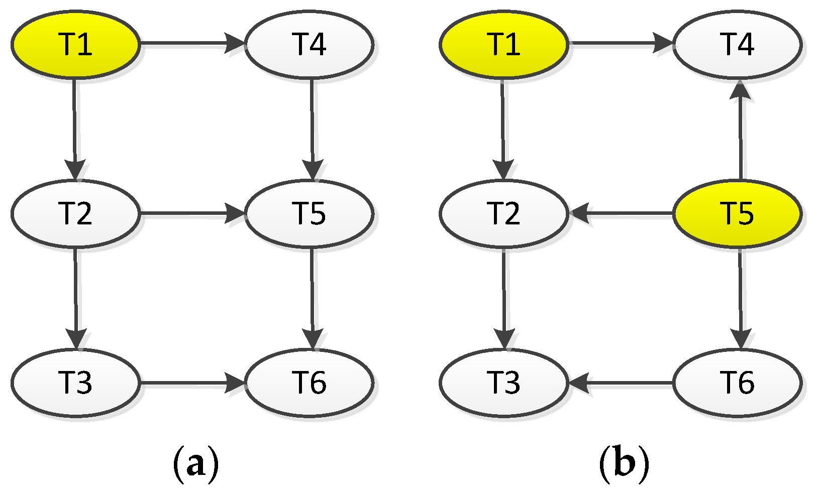
Figure 8a,b display the BNs for modeling the fire spread in the tank farm given a single fire at T1 (relevant to Scenario 1 and 2) and two separate fires at T1 and T5 (relevant to Scenario 3), respectively. To help distinguish between the graph theoretic approach and the BN approach, the nodes in the BNs have been presented as ellipse. For the sake of clarity, the conditional probability table of node T5 in Figure 8a given its immediate parents T2 and T4 have been reported in

Table 4. Conditional probability table of T5 in Figure 8a.

T2	T4	T5
		Fire	Safe
Fire	Fire	P24	1-P24
Fire	Safe	P2	1-P2
Safe	Fire	P4	1-P4
Safe	Safe	0	1

.

As previously mentioned, the escalation probabilities in Table 4 can be calculated using probit functions [10,33]. Since the aim of the present study is to identify an optimal firefighting strategy based on relative importance of the storage tanks not their exact escalation probabilities, and because the tanks are of the same type and dimension, we calculate the escalation probabilities using a linear relationship:

$$P_i=1-\frac{15}{Q_i}$$

(6)

where P_i is the escalation probability of the atmospheric tank exposed to a heat radiation of intensity Q_i (kW/m²). Further, the numerator 15 in Equation (6) denotes the escalation threshold of atmospheric tanks [33]. Accordingly, the escalation probabilities of tank T5 in Table 4 could be calculated as P₂ = 1 − 15/20 = 0.25, P₄ = 1 − 15/40 = 0.625, and P₂₄ = 1 − 15/(20 + 40) = 0.75. It should be noted that the escalation probability given in Equation (6) is merely for illustrative purposes and is not aimed at replacing the probit functions.

The BN in Figure 8a can be extended to influence diagrams in Figure 9a,b in order to identify optimal firefighting strategies in Scenarios 1 and 2. In Figure 9a, for instance, the decision node incorporates eight firefighting strategies (decision alternatives) in form of Ti–Tj (for i = 1, 2 and j = 3, 4, 5, 6), standing for suppression of Ti and cooling of Tj. For example, the decision alternative T1–T3 indicates that the corresponding firefighting strategy involves the suppression of T1 and the cooling of T3. The dashed arcs from T1 and T2 to the decision node implies that the firefighting strategies would be conditioned to the observation of fires at T1 and T2.

The impact of the decision alternatives on the nodes of the influence diagram can be reflected by making modifications to the conditional probability tables (escalation probabilities) of the exposed tanks which are being influenced by the decision node. Part of the modified conditional probability table of T5 in Figure 9a has been illustrated in

Table 5. Part of the conditional probability table of T5 in Figure 9a.

Decision	T2	T4	T5
			Fire	Safe
T1–T3	Fire	Fire	P24	1-P24
T1–T4	Fire	Fire	P2	1-P2
T1–T5	Fire	Fire	0	1
T1–T6	Fire	Fire	P24	1-P24
T2–T3	Fire	Fire	P4	1-P4
T2–T4	Fire	Fire	0	1
T2–T5	Fire	Fire	0	1
T2–T6	Fire	Fire	P4	1-P4

. It should be noted that some entries in Table 5 might seem contradictory at first glance if the entire influence diagram is not taken into consideration.

For example, on the second row of Table 5, the decision T1–T4 denotes the cooling of T4 (i.e., T4 is safe and is being cooled to keep safe) whereas the state of T4 is Fire. Such contradiction can be justified if it is noted that under the same decision alternative the probability of T4 being on fire would be equal to zero (the arc from “Decision” to T4). As such, the escalation probability of T5 (2nd row in Table 5) is only due to the heat radiation received from T2; thus, P(T5 = Fire | d = T1 − T4, T2 = Fire, T4 = Fire) = P₂. Following the same approach, the BN in Figure 8b can be extended to the influence diagram in Figure 9c to identify the optimal firefighting strategy in the event of Scenario 3.

In the influence diagrams shown in Figure 9a–c, the node “Utility” has been connected to the still-safe storage tanks so that only the further damage caused by the fire spread can be taken into account in the decision making. Since the storage tanks are identical, we have assumed that a damaged storage tank (due to fire spread) is associated with a disutility of −10.0 while the disutility of a safe tank is 0.0. For example, in Figure 9a, U(T3 = Safe, T4 = Fire, T5 = Fire, T6 = Safe) = −20.0.

Implementing the influence diagrams in GeNIe software [37], the expected disutility of firefighting strategies (decision alternatives) are reported in

Table 6. Expected (Exp) disutility of firefighting strategies for fire scenarios.

Figure 9a: Scenario 1		Figure 9b: Scenario 2		Figure 9c: Scenario 3
Decision	Exp. Disutility	Decision	Exp. Disutility	Decision	Exp. Disutility
T1–T3	−3.04	T4_T3	−3.04	T1–T2	−8.44
T1–T4	−7.67	T4_T5	−4.64	T1–T3	−9.80
T1–T5	−4.64	T4_T6	−6.00	T1–T4	−7.67
T1–T6	−6.00	T2_T3	−5.24	T1–T6	−6.84
T2–T3	−3.35	T2_T5	0.00	T5–T2	−2.20
T2–T4	0.00	T2_T6	−3.80	T5–T3	−6.00
T2–T5	−2.20			T5–T4	−5.24
T2–T6	−3.04			T5–T6	−7.44

. In Scenario 1, the optimal decision (attributed to the lowest disutility) would be to suppress T2 and to cool T4 (see the result of the graph theoretic approach in Section 3.2.1). Likewise, in the event of Scenario 2, the suppression of T2 and the cooling of T5 would be the optimal strategy (see the result of the graph theoretic approach in Section 3.2.2) and the vice versa in Scenario 3 (see the result of the graph theoretic approach in Section 3.2.3). As can be seen, the results obtained from the influence diagrams are in complete agreement with those obtained from the graph theoretic approach in the previous sections. For the sake of clarity, the lowest amount of loss (the lowest absolute amount of expected disutility) in each scenario and their corresponding decisions are depicted with bold numbers in Table 6.

4. Application of the Methodology

The graph theoretic methodology can effectively be applied to large oil terminals where the number of units could impede the application of influence diagrams. Application of influence diagram to such facilities faces two challenges: (i) for each fire spread scenario which may initiate from a single unit or multiple units a separate influence diagram should be developed, and (ii) due to complicated interactions between the units during fire spread the size of conditional probability tables can grow exponentially and thus becomes intractable.

Figure 10a displays an oil terminal comprising fifteen tanks of gasoline with diameter of D = 27 m, height of H = 15 m, and capacity of 9000 m³. Considering tank fires as the most likely fire events, possible fire spread patterns have been presented as the directed graph in Figure 10b.

Two fire scenarios are considered:

• Scenario A: fire starts at T7 and escalates to T6 and T12, and
• Scenario B: fire starts simultaneously at T4, T10, and T12.

It is also assumed that the plant’s firefighting team is equipped with three firefighting trucks, of which two can be used to suppress burning tanks while the third one to cooling one exposed tank. Without replicating the methodology steps, the out-closeness scores calculated sequentially by isolating the suppressed and cooled tanks are reported in

Table 7. Identification of optimal firefighting strategies based on the out-closeness scores.

Tank	Scenario A		Scenario B
	T6, T7 & T12 Are on Fire	T7 & T12 Are Suppressed	T4, T10 & T12 Are on Fire	T4 & T12 Are Suppressed
T1	0.077	0.077	0.077	0.067
T2	0.077	0.077	0.077	0.067
T3	0.077	0.077	0.077	0.067
T4	0.083	0.083	0.219	0.067
T5	0.089	0.089	0.126	0.067
T6	0.095	0.095	0.136	0.071
T7	0.114	0.067	0.144	0.077
T8	0.107	0.067	0.151	0.152
T9	0.110	0.067	0.152	0.151
T10	0.109	0.067	0.147	0.147
T11	0.105	0.067	0.136	0.136
T12	0.117	0.067	0.171	0.067
T13	0.109	0.067	0.149	0.149
T14	0.109	0.067	0.144	0.144
T15	0.107	0.067	0.133	0.133

. As can be noted, the following firefighting strategies could be identified as the optimal ones for each fire scenario:

• For Scenario A: suppress T7 and T12, and cool T5,
• For Scenario B: suppress T4 and T12, and cool T8.

For the sake of clarity, the out-closeness scores of the critical units are depicted with bold numbers in Table 7. Besides, the modified graphs of Scenarios A and B before and after implementation of the firefighting strategies have been depicted in Figure 11. As can be seen from Figure 11b, in the case of Scenario A, the suppression of T7 and T12 and the cooling of T5 completely prevent from the fire spread in the tank terminal. On the other hand, in the case of Scenario B, the suppression of T4 and T12 and the cooling of T8 do not entirely prevent from but significantly limit the fire spread.

5. Conclusions

In the present study, we developed methodologies based on graph theory and influence diagrams for optimal firefighting of fires at oil terminals under insufficient firefighting resources. Modeling fire spreads as a directed graph, we demonstrated that suppression of burning units with the highest out-closeness scores would be the most effective fire suppression policy. Removing the suppressed units from the graph, and recalculating the out-closeness scores of the remaining units, it was demonstrated that cooling of exposed units with the highest updated out-closeness scores would be the most effective cooling policy. As such, simultaneous suppressing and cooling of burning and exposed units—as many as the firefighting resources allow—based on sequential calculation of out-closeness scores can be adopted as an optimal firefighting strategy.

In the case of oil and gas facilities which comprise a variety of units of different type and size, the developed influence diagram outperforms the graph theoretic approach by facilitating the incorporation of different escalation probabilities and damage (disutility) values. In the case of large facilities with more or less similar units, however, the graph theoretic approach outdoes the influence diagram. This is mainly because the large number of units can make the development of influence diagrams and identification of conditional probabilities and utility values very time-consuming.

References

1. BBC. How the Buncefield Fire Happened. 2010. Available online: http://www.bbc.com/news/uk-10266706 (accessed on 8 October 2018).
2. U.S. Chemical Safety Board (CSB). Caribbean Petroleum Refining Tank Explosion and Fire. 2015. Available online: http://www.csb.gov/caribbean-petroleum-refining-tank-explosion-and-fire (accessed on 8 October 2018).
3. REUTERS. Fuel Tanks on Fire at Storage Facility in SANTOS, Brazil. 2015. Available online: https://www.reuters.com/article/us-brazil-fire-fueltanks/fuel-tanks-on-fire-at-storage-facility-in-santos-brazil-idUSKBN0MT1SU20150402 (accessed on 22 May 2018).
4. REUTERS. Fire Extinguished at Fuel Oil Storage Tank in Singapore. 2018. Available online: https://www.reuters.com/article/us-singapore-energy-fire/fire-extinguished-at-fuel-oil-storage-tank-in-singapore-idUSKBN1GX05N (accessed on 22 May 2018).
5. Vilchez, A.J.; Montiel, H.; Casal, J.; Arnaldos, J. Analytical expressions for the calculation of damage percentage using the probit methodology. J. Loss Prev. Process. Ind. 2001, 14, 193–197. [Google Scholar] [CrossRef]
6. Liu, Y. Thermal Buckling of Metal Oil Tanks Subject to an Adjacent Fire. Ph.D. Thesis, University of Edinburgh, Edinburgh, UK, 2011. [Google Scholar]
7. Mansour, K. Fires in Large Atmospheric Storage Tanks and Their Effect on Adjacent Tanks. Ph.D. Thesis, Loughborough University, Loughborough, UK, 2012. [Google Scholar]
8. Reniers, G.; Cozzani, V. Domino Effects in the Process Industries; Elsevier: Kidlington, UK, 2013. [Google Scholar]
9. Cozzani, V.; Gubinelli, G.; Antonioni, G.; Spadoni, G.; Zanelli, S. The assessment of risk caused by domino effect in quantitative area risk analysis. J. Hazard. Mater. 2005, A127, 14–30. [Google Scholar] [CrossRef] [PubMed]
10. Landucci, G.; Gubinelli, G.; Antonioni, G.; Cozzani, V. The assessment of the damage probability of storage tanks in domino events. Accid. Anal. Prev. 2009, 41, 1206–1215. [Google Scholar] [CrossRef] [PubMed]
11. Abdolhamidzadeh, B.; Abbasi, T.; Rashtchian, D.; Abbasi, S.A. A new method for assessing domino effect in chemical process industry. J. Hazard. Mater. 2010, 182, 416–426. [Google Scholar] [CrossRef] [PubMed]
12. Khakzad, N.; Khan, F.; Amyotte, P.; Cozzani, V. Domino effect analysis using Bayesian networks. Risk Anal. 2013, 33, 292–306. [Google Scholar] [CrossRef] [PubMed]
13. Khakzad, N.; Reniers, G. Using graph theory to analyze the vulnerability of process plants in the context of cascading effects. Reliab. Eng. Syst. Saf. 2015, 143, 63–73. [Google Scholar] [CrossRef] [Green Version]
14. Landucci, G.; Argenti, F.; Tugnoli, A.; Cozzani, V. Quantitative assessment of safety barrier performance in the prevention of domino scenarios triggered by fire. Reliab. Eng. Syst. Saf. 2015, 143, 30–43. [Google Scholar] [CrossRef]
15. Nash, P. Fire Protection of Flammable Liquid Storages by Water Spray and Foam; Fire Research Station: Borehamwood, UK, 1975. [Google Scholar]
16. Persson, H.; Lönnermark, A. Tank Fires: Review of Fire Incidents 1951–2003. BRANDFORSK Project 513-021. SP Swedish National Testing and Research Institute SP Rapport 2004: 14. Available online: https://www.msb.se/Upload/Insats_och_beredskap/Brand_raddning/Oljedepa/Cisternrapport%202004_14.pdf (accessed on 22 May 2018).
17. Lang, X.; Liu, Q.; Gong, H. Study of firefighting systems to extinguish full surface fire of large scale floating roof tanks. Procedia Eng. 2011, 11, 189–195. [Google Scholar]
18. Forell, B.; Peschke, J.; Einarsson, S.; Röwekam, M. Technical reliability of active fire protection features—Generic database derived from German nuclear power plants. Reliab. Eng. Syst. Saf. 2016, 145, 277–286. [Google Scholar] [CrossRef]
19. D’Amico, M. Risk Based Fire Protection Strategy in Crude Oil Storage Facilities. International Fire Protection Magazine E-Newswire 2015, Issue 64. Available online: https://ifpmag.mdmpublishing.com/risk-based-fire-protection-strategy-in-crude-oil-storage-facilities/ (accessed on 8 October 2018).
20. Khakzad, N. Which fire to extinguish first? A risk-informed approach to emergency response in oil terminals. Risk Anal. 2018, 38, 1444–1454. [Google Scholar] [CrossRef] [PubMed]
21. National Fire Protection Association (NFPA). Standard for Low, Medium, and High-Expansion Foam; NFPA: Quincy, MA, USA, 2002. [Google Scholar]
22. Centre for Chemical Process Safety (CCPS). Guidelines for Fire Protection in Chemical, Petrochemical, and Hydrocarbon Processing Facilities; Wiley-AIChE: New York, NY, USA, 2003. [Google Scholar]
23. API RP 2001. Fire Protection in Refineries—Candidate Ballot Draft 8-3-2011. 2011. Available online: http://ballots.api.org/sfp/ballots/docs/RP2001BallotDraft9thEd.pdf (accessed on 8 October 2018).
24. Newman, M. Networks: An Introduction; Oxford University Press, Inc.: New York, NY, USA, 2010. [Google Scholar]
25. Watts, D.J.; Strogatz, S.H. Collective dynamics of ‘small-world’ networks. Nature 1998, 393, 440–442. [Google Scholar] [CrossRef] [PubMed]
26. Albert, R.; Jeong, H.; Barabasi, A.L. Error and attack tolerance of complex networks. Nature 2000, 406, 378–381. [Google Scholar] [CrossRef] [PubMed]
27. Latora, V.; Marchiori, M. Efficient behavior of small-world networks. Phys. Rev. Lett. 2001, 87, 1–4. [Google Scholar] [CrossRef] [PubMed]
28. Yazdani, A.; Appiah Otoo, R.; Jeffery, P. Resilience enhancing expansion strategies for water distribution systems: A network theory approach. Environ. Model. Softw. 2011, 26, 1574–1582. [Google Scholar] [CrossRef]
29. Di Nardo, A.; Di Natale, M. A heuristic design support methodology based on graph theory for district metering of water supply networks. Eng. Optim. 2011, 43, 193–211. [Google Scholar] [CrossRef]
30. Huang, H.; Li, K. Train timetable optimization for both a rail line and a network with graph-based approaches. Eng. Optim. 2017, 49, 2133–2149. [Google Scholar] [CrossRef]
31. Pearl, J. Probabilistic Reasoning in Intelligent Systems; Morgan Kaufmann: San Francisco, CA, USA, 2014. [Google Scholar]
32. Neapolitan, R. Learning Bayesian Networks; Prentice Hall, Inc.: Upper Saddle River, NJ, USA, 2003. [Google Scholar]
33. Cozzani, V.; Gubinelli, G.; Salzano, E. Escalation thresholds in the assessment of domino accidental events. J. Hazard. Mater. 2006, 129, 1–21. [Google Scholar] [CrossRef] [PubMed]
34. ALOHA. US Environmental Protection Agency, National Oceanic and Atmospheric Administration. Available online: http://www.epa.gov/OEM/cameo/aloha.htm (accessed on 8 October 2018).
35. Large Atmospheric Storage Tank Fires (LASTFIRE). LASTFIRE Boilover Lessons, Issue 3, December 2016. Available online: http://www.lastfire.org.uk/refmatpapers.aspx?id=5 (accessed on 8 October 2018).
36. Csardi, G.; Nepusz, T. The igraph software package for complex network research. Int. J. Complex Syst. 2006, 1695, 1–9. [Google Scholar]
37. GeNIe. Decision Systems Laboratory, University of Pittsburg. Available online: https://www.bayesfusion.com (accessed on 8 October 2018).
Figure 1. (a) Schematic of a gasoline storage terminal. (b) Mutual heat radiation intensities (kW/m2) in the event of tank fires. (c) Potential fire spread paths in the terminal as a directed graph.
Energies 11 03101 g001
Figure 2. Optimal firefighting strategy for Scenario 1. (a) T1 and T2 are on fire. (b) T1 is on fire while T2 is suppressed. (c) T1 is on fire, T2 is suppressed, and T4 is cooled.
Energies 11 03101 g002
Figure 3. Non-optimal firefighting strategy for Scenario 1. (a) T1 and T2 are on fire. (b) T1 is suppressed while T2 is on fire. (c) T1 is suppressed, T2 is on fire, and T5 is cooled.
Energies 11 03101 g003
Figure 4. Optimal firefighting strategy for Scenario 2. (a) T1, T2, and T4 are all on fire. (b) T1 and T4 are on fire while T2 is suppressed. (c) T1 and T4 are on fire, T2 is suppressed, and T5 is cooled.
Energies 11 03101 g004
Figure 5. Non-optimal firefighting strategy for Scenario 2. (a) T1, T2, and T4 are all on fire. (b) T1 and T2 are on fire, and T4 is suppressed. (c) T1 and T2 are on fire, T4 is suppressed, and T6 is cooled.
Energies 11 03101 g005
Figure 6. Optimal firefighting strategy for Scenario 3. (a) T1 and T5 are on fire. (b) T1 is on fire while T5 is suppressed d. (c) T1 is on fire, T5 has been suppressed, and T2 is cooled.
Energies 11 03101 g006
Figure 7. Non-optimal firefighting strategy for Scenario 3. (a) T1 and T5 are on fire. (b) T1 has been suppressed while T5 is on fire. (c) T1 has been suppressed, T5 is on fire, and T3 is cooled.
Energies 11 03101 g007
Figure 8. Application of Bayesian network (BN) to modelling fire domino effect in the terminal. (a) The domino effect starts from T1. (b) The domino effect starts from T1 and T5.
Energies 11 03101 g008
Figure 9. Influence diagrams to identify the optimal firefighting strategies in (a) Scenario 1, (b) Scenario 2, and (c) Scenario 3.
Energies 11 03101 g009
Figure 10. (a) An oil terminal. (b) Possible fire spread scenarios as a directed graph.
Energies 11 03101 g010
Figure 11. (a) Fire spread paths in the case of Scenario A. (b) Fire spread paths after the implementation of firefighting in the case of Scenario A. (c) Fire spread paths in the case of Scenario B. (d) Fire spread paths after the implementation of firefighting in the case of Scenario B.
Energies 11 03101 g011