Article

Distributed Thermal Response Tests Using a Heating Cable and Fiber Optic Temperature Sensing

1
Institut National de la Recherche Scientifique, Centre Eau Terre Environnement, Québec, QC G1K 9A9, Canada
2
Universidad de Medellín, Programa de Ingeniería Ambiental, Medellín 050026, Colombia
3
BRGM, Georesources Division, 45060 Orléans CEDEX 2, France
4
Univ Rennes, CNRS, Géosciences Rennes—UMR 6118, F-35000 Rennes, France
5
École de Technologie Supérieure, Département de génie mécanique, Montréal, QC H3C 1K3, Canada
*
Authors to whom correspondence should be addressed.
Energies 2018, 11(11), 3059; https://doi.org/10.3390/en11113059
Submission received: 25 July 2018 / Revised: 19 October 2018 / Accepted: 2 November 2018 / Published: 7 November 2018
(This article belongs to the Special Issue Geothermal Energy: Utilization and Technology 2018)

Abstract

:
Thermal response tests are used to assess the subsurface thermal conductivity to design ground-coupled heat pump systems. Conventional tests are cumbersome and require a source of high power to heat water circulating in a pilot ground heat exchanger. An alternative test method using heating cable was verified in the field as an option to conduct this heat injection experiment with a low power source and a compact equipment. Two thermal response tests using heating cable sections and a continuous heating cable were performed in two experimental heat exchangers on different sites in Canada and France. The temperature evolution during the tests was monitored using submersible sensors and fiber optic distributed temperature sensing. Free convection that can occur in the pipe of the heat exchanger was evaluated using the Rayleigh number stability criterion. The finite and infinite line source equations were used to reproduce temperature variations along the heating cable sections and continuous heating cable, respectively. The thermal conductivity profile of each site was inferred and the uncertainly of the test was evaluated. A mean thermal conductivity 15% higher than that revealed with the conventional test was estimated with heating cable sections. The thermal conductivity evaluated using the continuous heating cable corresponds to the value estimated during the conventional test. The average uncertainly associated with the heating cable section test was 15.18%, while an uncertainty of 2.14% was estimated for the test with the continuous heating cable. According to the Rayleigh number stability criterion, significant free convection can occur during the heat injection period when heating cable sections are used. The continuous heating cable with a low power source is a promising method to perform thermal response tests and further tests could be carried out in deep boreholes to verify its applicability.

1. Introduction

Ground coupled heat pump systems, made of a ground heat exchanger (GHE) and a heat pump, are recognized as an efficient and environmentally friendly technology to cool and heat residential and commercial buildings. The thermal conductivity and the borehole thermal resistance are required to design such systems considering that an accurate estimation of these properties has a direct impact on their efficiency and cost [1,2].
Thermal response tests (TRTs) have been proposed by Mogensen [3] as an in situ method to assess the subsurface thermal conductivity and the borehole thermal resistance. The first mobile TRT devices were developed by Eklöf and Gehlin [4] and Austin III [5] at Luleå Technical University and Oklahoma State University, respectively, and historic reviews of the TRT development were published by Gehlin [6], Sanner et al. [7] and Spitler and Gehlin [8]. During a conventional test, the fluid circulating in the GHE is heated using an electrical element in the TRT ring to reproduce heat transfer phenomena occurring in the GHE. Inlet and outlet temperatures along with flow rate are recorded and then analyzed to determine the bulk subsurface thermal conductivity over the length intercepted by the borehole [9,10]. TRT analysis is usually performed using the infinite line source model, an analytical solution to the heat conduction equation [11,12]. This one-dimensional conductive heat transfer solution describes the mean temperature increment at a radial distance from an infinite source of heat having a constant heat flow rate and assuming a constant temperature at an infinite radial distance from the source.
Conventional TRT requires a source of high power (50–80 W·m−1 [13]) to heat the water circulating in the GHE and generate a temperature difference of 3–7 °C at the inlet and outlet of the GHE, reproducing the operation of a geothermal system. The bulk thermal conductivity is estimated over the length intercepted by the borehole [14]. Depending on the site properties, the estimated bulk thermal conductivity can be affected by the ground heterogeneity [15] and groundwater flow [16,17]. The use of fiber optic distributed temperature sensing (FO-DTS), a technology to monitor temperature at high frequency and spatial resolution [18], was proposed by Fujii et al. [15,19] to measure the vertical temperature profile during TRT as an alternative method to assess the vertical distribution of the ground thermal conductivity and associated ground heterogeneity. Subsequently, fiber optic cables have been used to validate analytical models of the vertical temperature evolution [20] and to measure borehole wall temperatures [21] during TRTs. FO-DTS and a heat trace cable was additionally used by Freifeld et al. [22] to estimate the ground thermal conductivity as a function of depth and to infer ground surface temperature history.
To reduce the power requirements of TRTs, which is one of the important expenses estimated to be 10–30% of the total test cost [23], and to evaluate the thermal conductivity as a function of depth, an alternative method to perform TRTs using heating cables and submersible temperature sensors was proposed by Raymond et al. [24,25]. In locations where the ground is heterogeneous, the GHE can preferentially be drilled into lithological units with a high thermal conductivity [19]. Obtaining the vertical distribution of the thermal conductivity may allow defining the most advantageous drilling conditions for the GHE in addition to better constrain the simulation of the system that can consider subsurface heterogeneity. Moreover, tests with heating cables are not affected by temperature variation at surface, such as atmospheric temperature changes and solar radiations, commonly influencing the heat injection rates of conventional TRT taking place at surface [25]. The proposed method uses a cable standing in the water column of the GHE pipe to heat the ground, with several advantages, such as avoiding water circulation, removing the adverse effect of surface temperature fluctuations, reducing the required heat injection rate and simplifying the field manipulations. Two types of cable were used to perform the tests: a continuous heating cable and interchanging sections of heating and non-heating cable. The heat injection rate of heating cables used for previous tests varied from 20 to 40 W·m−1 [24,23] and the required power of less than 1 kW was supplied by connecting the TRT unit to the electrical grid [24]. Tests with a continuous heating cable wete achieved in boreholes having a depth of approximately 30 m, while boreholes with more than 100 m in length have been the subject of tests with heating sections to keep a low power requirement [26].
The test analysis conducted when using the continuous heating cable is similar to that of a conventional TRT, based on the infinite line source solution to reproduce the observed temperature increments in the GHE. A finite heat source solution must be used for the analysis of a test with heating cable sections to adequately reproduce observed temperatures along the heating sections that can be 1–2 m in length [24]. These mathematical solutions are based on the assumption of conductive heat transfer only, while natural convection can occur in the standing water column of the GHE pipe, especially near the limits of the heating and non-heating sections due to the temperature gradient created within the pipe upon heat injection. Numerical simulations conducted by Raymond and Lamarche [23] and small-scale field experiments with one heating section [27] indicated that perforated plastic disks located between heating and non-heating sections can reduce convective heat transfer. It was, therefore, suggested to investigate the effect of natural convection during full-scale TRT experiments conducted in the field with continuous and heating cable sections.
The objectives of this work were to better understand free convection and conduction heat transfer mechanisms occurring during a TRT with a heating cable to estimate the subsurface thermal conductivity and its uncertainly, as well as to assess the effect of perforated plastic disks to reduce free convection when heating cable sections are used. Two TRTs using heating cables and FO-DTS were conducted at two experimental sites in Quebec City, Canada, and Orléans, France, with vertical closed-loop heat exchangers. A first test was done with ten heating sections in a 100 m borehole using a heat injection rate of ~40 W·m−1 while, at the other site, a second test was achieved in a borehole of equivalent length with a continuous heating cable and a heat injection rate of less than ~10 W·m−1. This paper describes first heating cable TRTs combined with FO-DTS and a first continuous heating cable TRT in a long borehole with a low heat injection rate. Conventional TRT with water circulation was previously conducted at both sites and the results were used for comparison purposes. The Rayleigh number stability criterion, a methodology to evaluate convective heat transfer in vertical groundwater wells proposed by Love et al. [28], was applied to assess convective heat transfer during the tests. FO-DTS technology used to monitor temperature in boreholes at high frequency and spatial resolution along a fiber-optic cable [18] provided the information needed to evaluate the Rayleigh number stability criterion. Thermal conductivity profiles were estimated using the infinite and finite heat source solution depending on the heating cable used and an uncertainty analysis of each test was performed.

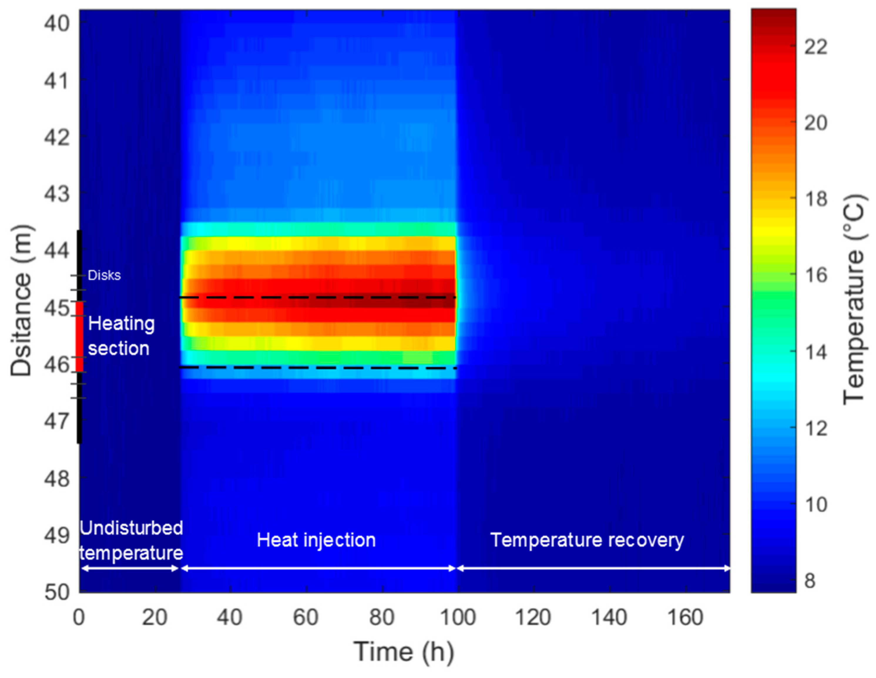
2. Field Test Methodology

The TRT with heating cable sections was carried out at the Laboratories for scientific and technological innovation in environment of the Institut national de la recherche scientifique, located in Quebec City, Canada. A GHE made of a single U-pipe was used to perform the test to a depth of ~100 m. The borehole intercepts backfill material down to a depth of 2 m, followed by 8 m of clay and then shale constituting the host rock (Figure 1a). This last geological unit is the Les Fonds Formation of the Sainte-Rosalie Group in the St. Lawrence Lowland sedimentary basin [29]. The groundwater levels inside the borehole was approximately 2 m depth.
The second TRT with a continuous heating cable was carried out at the experimental geothermal test facility of the Bureau de Recherches Géologiques et Minière in Orléans, France. A GHE made of a double-U pipe was used for the test to a depth of ~100 m. This borehole intercepted 8 m of sand and clay of the Sologne Basin succeeded by limestone formations (Figure 1b), mainly Calcaire de Pithiviers and Calcaire du Gatinais [30].
The cable used for the test in Québec City is made of interchanging heating and no heating sections with length of 1.20 and 8.60 m, respectively (Figure 2a), while that for the test in Orléans was continuous (Figure 2b). The same field test methodology was applied to both sites, but the heat injection rate was adapted according to heating cable design to achieve a low-power requirement.
The equipment required to perform the tests consists of the heating cable assembly, a junction box to link the cable to the power supply (Figure 3), and submersible sensors to measure and record the temperature during the test. The junction box is composed of an automated switch to start and stop the heat injection, a voltage regulator, a power meter with an accuracy of ±0.02 W to monitor the power induced and circuit breakers to protect the electric circuits of the cable assembly and the power meter [25]. Additionally, when heating cable sections are used, perforated plastic disks are needed. Four disks separated by about 10 cm and defining the active heating length for analysis were installed at the interface between the heating and non-heating sections to reduce the possible convective heat transfer.
The temperature was measured for both tests using submersible sensors and a fiber-optic cable. The submersible sensors are DST-centi temperature data loggers with an accuracy of ±0.10 °C and a resolution of 0.032 °C made by Star-Oddi. The FO-DTS system used for the test in Québec City consisted of a BruSens fiber optic cable of 250 m length connected to a Silixa XT-DTS control unit in double-ended configuration with 2 km range [31]. This 3.80 mm diameter fiber optic sensing cable, armored with stainless steel, has a fast thermal response which allows for recording temperature changes efficiently. Two cable sections of 20 m long were placed in an ambient (37.40 °C) and cold (0.30 °C) temperature bath, respectively, to calibrate the DTS unit. A Starmon mini probe (±0.025 °C) and a RBRduet probe (±0.002 °C) were used in the bath to record the temperature for calibration purpose. The FO-DTS used in Orléans for the second test was an Orxy DTS in double-ended configuration with a temperature resolution of ±0.05 °C [30]. The temperature measured with the fiber optic was corrected using a calibration bath at 0 °C.
In the first case, the submersible temperature sensors were placed in the middle of each heating section located approximately every 10 m, from 5 to 95 m depth. The fiber optic cable was attached to the cable assembly that was lowered in a pipe of the ground heat exchanger reaching a depth of 100 m. The FO-DTS system was configured to collect data every 60 s with a 25 cm sampling interval along the fiber optic cable while the submersible sensors recorded temperature every 10 min. The sampling interval of the temperature sensor and the fiber optic are different because the FO-DTS data are used to assess free convection during the TRT and the data from the submersible sensors is used to infer the thermal conductivity. The test started with a measure of the undisturbed subsurface temperature followed by heat injection at an average rate of 42.50 W·m−1, after which the thermal recovery was monitored. The double U-pipe heat exchanger in Orléans was equipped with a FO-DTS system that allows measuring the temperature in two of the pipes of the GHE. The test was implemented with a continuous heating cable of 95 m. The submersible temperature sensors were placed every 6 m, from 5.50 to 83.60 m depth, and the FO-DTS system was programed to collect data each meter, every 10 min. Due to the small pipe diameter, the heating cable and the fiber optic cables could not be placed in the same pipe. Thus, it was installed in other pipes located at 0.06 and 0.82 m from the pipes containing the fiber optic. The four pipes in this GHE are separated with spacers. The test started with the measurement of the undisturbed subsurface temperatures followed by heat injection at a rate of 9.90 W·m−1 and, finally, thermal recovery monitoring. A test with a heat injection rate below 10 W·m−1 was possible due to the improvement of temperature sensor resolution accomplished in recent years. Sensors with a resolution less than 0.05 °C are able to measure small temperature changes allowing to perform the tests with a low heat injection rate, which was difficult to achieve with previously available technologies.

3. Test Analysis

3.1. Thermal Conductivity Assessment

The test analysis was done with the line source solution for conductive heat transfer. Two variations of this solution were used according to the cable deployed to perform the test. Heating cable sections were represented as finite line sources, whereas the infinite line source was used for the continuous heating cable. The methodology to analyze the TRT with both types of cable was previously described by Raymond and Lamarche [23] and Raymond et al. [24].
The temperature data collected with the submersible sensors were used to estimate the thermal conductivity at the depth of each sensor. The recovery temperature increments (ΔT = TT0), defined as the increase of temperature with respect to the initial temperature T0, were reproduced with the analytical solutions using the temporal superposition principle to consider the recovery period where heat injection is zero. Numerical simulation results described by Raymond et al. [10] indicate that the temperature inside a slice of a borehole varies significantly according to the horizontal measurement location during the heat injection, making it necessary to consider the horizontal position of the temperature sensor to analyze the test. However, during the recovery period, the temperature becomes uniform and the position of the sensor does not influence the measurement. The horizontal position of the temperature sensor is difficult to determine; therefore, the thermal conductivity was estimated using only the late recovery temperatures at each depth. A linear heat source solution of finite length with a dimensionless g-function (Equation (1), [24,25]), which depends on the Fourier number (Fo), was used to analyze the test with heating sections:
Δ T = q 2 π λ s [ g ( F o , r h ) g ( F o , r h ) ]  
with
F o = α s ( t ) h 2  
and
F o = α s ( t t o f f ) h 2  
where q (W·m−1) is the heat injection rate per unit length; α s (m2 s−1) and λs (W·m−1·K−1) are the thermal diffusivity and conductivity of the subsurface, respectively; r (m) is the radial distance from the heat source; h (m) is the active heating length; and toff is the time when heat injection was stopped. The heat capacity of the subsurface was assumed based on the rock type identified with drill cuttings and it was also used to determine the thermal diffusivity ( α s ) and to compute Fourier’s number (Equations (2) and (3)). The heat injection rate q (W·m−1) for each heating section was assumed similar and determined according to Joule’s and Ohm’s laws:
q = R h I 2 n h  
where
R h = R t o t R n h  
and
R t o t = U I  
where R (Ohm) is the electric resistance, I (A) is the electrical current intensity, U (V) is the potential difference, n is the number of heating sections and h (m) is the length of the heating sections. The subscripts h, nh, and tot correspond, to the electrical resistance of the heating sections, of the non-heating sections and of the whole cable assembly, respectively.
The computed temperature increments of the late recovery period were matched with a non-linear solver [32] to the observed temperature increments by adjusting the thermal conductivity using a least-squared fit. The analysis of the temperature measurements recorded with the submersible data loggers was performed using a spreadsheet program developed by Raymond et al. [24].
The infinite line source equation was used for the second test with a continuous heating cable to evaluate the temperature increase during the late recovery period. TRT theories indicate that, after a sufficiently long heat injection time (t), the thermal conductivity can be estimated from the slope m of the graphic relating the temperature increases with the logarithmic time (Equation (7); [33]):
m = Δ T Δ ln ( t ) = q 4 π λ s  
A negative heat injection rate is introduced at time toff to simulate the recovery period [34] and temperatures are plotted as a function of a normalized time t/(ttoff) to find thermal conductivity with the slope method:
m = Δ T Δ ln ( t / t t o f f ) = q 4 π λ s  
The heat injection rate for the continuous heating cable was calculated from the electric potential difference and the electrical current intensity measurements (Equation (9)):
q = U I h  
where h (m) is now the total length of the continuous heating cable.

3.2. Uncertainty Analysis

An analysis of the different sources of error influencing the test results was performed to determine the uncertainty associated with the tests. Witte [35] proposed a methodology to evaluate the accuracy of the thermal conductivity estimated during TRT, considering the sources of error associated with the variables that are measured repeatedly during the test, measured once before or after the test or estimated independently. This methodology is based on the infinite line source equation, which is the model commonly used to analyze conventional TRT, and utilizes the standard deviation and the confidence interval as the measures of error. The general procedures described in the supplement 1 to the guide to the expression of uncertainty in measurement [36] and by Ellison and Williams [37] were used to calculate the propagation of errors.
The methodology proposed by Witte [35] was adapted in this study to calculate the uncertainly associated with the thermal conductivity estimated with both continuous and separated heating cable sections. The error analysis was applied to the finite line source equation for the test with heating cable sections while Witte [35] theory could directly be used for the test with the continuous cable relying on the infinite line source equation.
The combined error of the cable electrical resistivity for the heating sections assembly δRtot (Equation (10)), the electrical resistivity of the heating section δRh (Equation (11)) and the heat injection rate δq (Equation (12)) were determined using the accuracy of the individual parameters.
δ R t o t R t o t = ( δ V V ) 2 + ( δ I I ) 2  
δ R h = ( δ R t o t ) 2 + ( δ ( R n h L n h ) ) 2  
with
δ ( R n h L n h ) = R n h L n h ( δ R n h R n h ) 2 + ( δ L n h L n h ) 2  
δ q q = ( δ R h R h ) 2 + ( 2 δ I I ) 2 + ( δ h h ) 2  
Then, the methodology was adapted to estimate the uncertainty associated with the g-function used to calculate the temperature increments (Equation (1)). This equation was simplified by removing the constant value of 2π (Equation (14)) and the equation was modified defining a variable Z = g(Fo) ΔT−1 (Equation (15)), allowing for determination of the error associated with the analytical solution. The uncertainty δZ was determined over 95% confidence (Equation (16); [27]) by the generalization of the error estimation of non-linear regression (Equation (17)). From Equation (1), we have
Δ T = q λ s [ g ( F o ) g ( F o ) ] = q λ s f ( F o )  
q λ s = g ( F o ) Δ T = Z  
δ Z = 1.96   S Z  
The standard deviation of Sz was determined similarly to the standard deviation of a slope (Equation (17)), considering the standard deviation of the calculated temperature increases (ΔTc) and the measured temperature increases (ΔTm; Equation (18)).
S z = σ 2 S x g  
where
σ 2 = ( Δ T m Δ T c ) 2 n 2  
and
S x g = ( g g ¯ ) 2  
δ λ λ = ( δ q q ) 2 + ( δ Z Z ) 2  
In this set of equations, n represents the number of temperature data considered in the analysis, g is the finite heat source function calculated at each time at the depth of each temperature sensor and g ¯ is the mean value of the function at each depth (Sxg, Equation (19)). Finally, the uncertainty of the thermal conductivity estimation δλ was calculated considering the error of the heat injection rate and the error of Z (Equation (20)).
The accuracy of the individual parameters measured during the test with the continuous heating cable was used to calculate the combined error of the heat injection rate (Equation (21)) and the combined error of the slope of the graph relating the temperature increases with the logarithmic time δ m (Equation (22)). The uncertainty of the slope is expressed in terms of the regression residuals σ T 2 (Equation (23)) and the sum of the squared deviation from the sample mean (Sxt; Equation (24)). Finally, the uncertainty of the thermal conductivity δλ is calculated as a function of the error of the heat injection rate and the slope (Equation (25)).
δ q q = ( δ U U ) 2 + ( δ I I ) 2 + ( δ H H ) 2  
δ m = σ T 2 S x t  
where
σ T 2 = ( T m T c ) 2 n 2  
and
S x t = ( t t ¯ ) 2  
δ λ λ = ( δ q q ) 2 + ( δ m m ) 2  

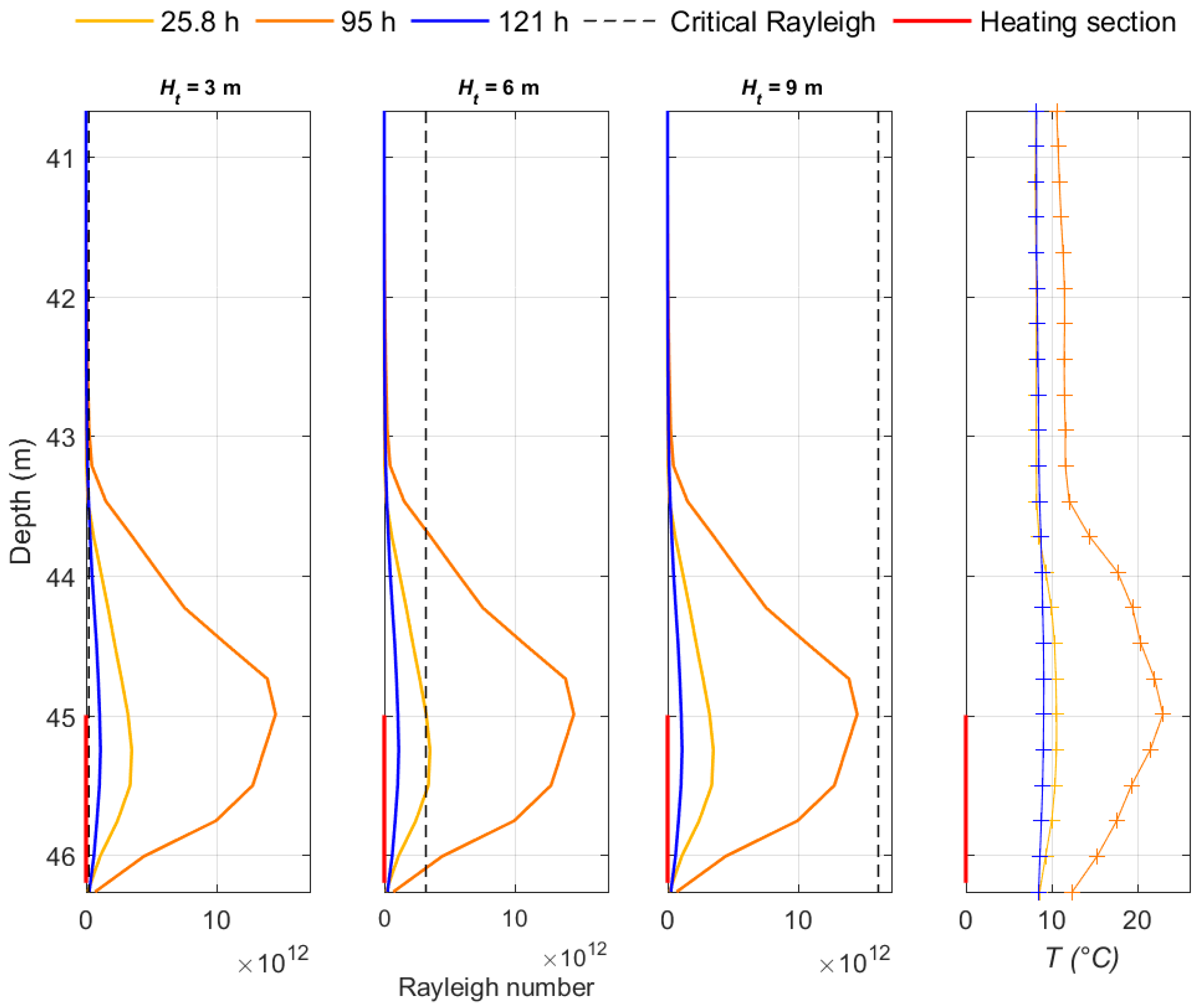
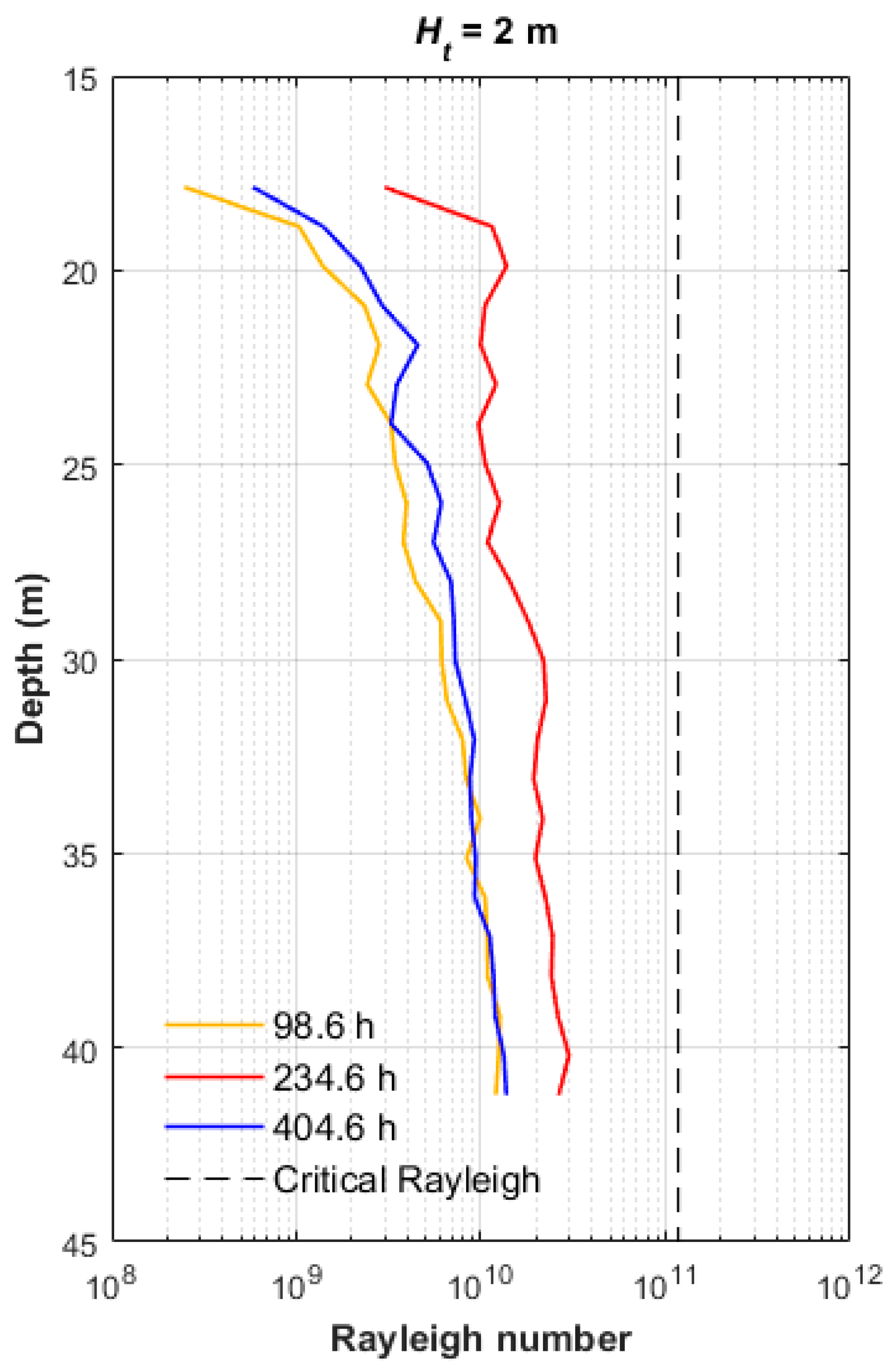
3.3. Free Convection Assessment Inside GHE Pipe

Love et al. [28] studied the diffusive transport induced by temperature variation in groundwater wells and formulated a Rayleigh number stability criterion to assess free convection in cylindrical wells. The stability criterion considers the well geometry and allows assessing the convection in a standing water column having temperature gradients between top and bottom. Free convection can be a dominant heat transfer mechanism when the Rayleigh number Ra calculated with Equation (26) exceeds a critical Rayleigh number Racr identified with Equation (27).
R a = G β H 3 Δ T ν α w  
where G (m·s−2) is the gravitational acceleration, β (K1) is the thermal expansion coefficient of the fluid, H (m) is the height of the water column, ΔT (°C) is the difference in temperature between the top and the bottom of the system, ν (m2·s−1) is the fluid cinematic viscosity and αw (m2·s−1) is the fluid thermal diffusivity. The critical Raleigh number computed for comparison is determined according to the cylinder geometry:
R a c r = 215.6 r a 4 ( 1 + 3.84 r a 2 )  
with
r a = r H t  
where r (m) is the well radius and Ht (m) is the height of the water column. The critical Rayleigh number is therefore a function of the well aspect ratio ra (-) only and an increment in the well aspect ratio results in a reduction of the Racr value [28].
The Rayleigh number stability criterion was proposed by Love et al. [28] to assess convection in groundwater wells in the presence of a geothermal gradient. In this study, the stability criterion was used to evaluate convection in GHE pipe where heat is injected using heating cables. Therefore, a similar approach based on the Rayleigh number stability criterion was applied to a system composed by a vertical pipe filled with water, where the temperature gradient is not uniform. Thus, Ht was defined as a critical length along the heating cable, rather than the well depth considered for groundwater well with a geothermal gradient. Nevertheless, defining a representative value for this variable is complicated because the critical Rayleigh number depends on the well aspect ratio. Increasing the well aspect ratio (larger radius and shorter height) results in a reduction of the critical Rayleigh number. Consequently, three different values of Ht were defined to evaluate its influence on the results of Rayleigh number stability criterion assessment.
A segment of 5.60 m of the cable assembly in the GHE was used to evaluate convection near a typical heating section. The segment is formed by a section of 4.40 m of non-heating cable located above a heating cable section of 1.20 m. The FO-DTS was used to determine ΔT in Equation (26) and compute the actual Raleigh number at different heights of the water column in the pipe varying over a range of 0.25–5.80 m to verify the Rayleigh number stability criterion.
The critical Rayleigh number was calculated for the pipe radius (r = 1.72 cm) and a critical length Ht of 3.00, 6.00 and 9.00 m. These values represent the mean height of the water column used to calculate actual Rayleigh numbers, the length of the maximum temperature difference between heating and non-heating sections and the total length of a system of a single heating and a non-heating section, respectively.
In the tests with a continuous cable, free convection is not expected because the heat injection rate is roughly uniform along the cable. Nevertheless, the Rayleigh criterion was evaluated to verify the absence of this effect. The shortest section showing the maximum temperature difference was selected, avoiding the first 5 m near the surface where the ambient temperature had an influence on the temperature measured in the pipe during the TRT. The criterion was evaluated between 18 m depth (minimal temperature of 12.30 °C) and 42 m depth (maximal temperature of 16.30 °C).
The actual Rayleigh numbers were computed considering a water column varying from 1 to 24 m. The pipe had a radius 1.31 cm and the critical Rayleigh number was first evaluated using a minimal critical length of 2 m. This value was defined as the minimal length because the sampling resolution of the fiber optic data was 1 m.

4. Results

The fiber optic measurements allowed visualizing the temperature evolution in the GHE during the whole test to better illustrate and understand heat transfer mechanisms. The undisturbed temperature was monitored during 26 h for the test in Québec City. Then, heat was injected for a period of 73 h (from 26 h to 99 h) and thermal recovery was monitored during the following 70 h, from 99 to 169 h (Table 1 and Figure 4). The total energy consumption during the test was 71.75 kWh and the average potential difference and electrical current intensity were 113 V and 8.7 A, respectively. The maximum temperature increase reached at the depth of each heating section was variable. Those differences are related to the variation in the subsurface thermal conductivity. High temperature increments at the depth of a heating section indicate a low subsurface thermal conductivity and a slight temperature increase corresponds to a greater thermal conductivity. The electric current during the field tests was fixed with a variable transformed allowing to reduce changes in heat injection rates. However, the heat injection rate was affected by the variation of the current intensity of the electrical grid. Local variation in the heat injection rate also in turn influenced the temperature increases. This effect was attenuated by analysis of recovery temperature measurements, where we know that heat injection is zero.
The distributed temperature measurement reveals an increase of approximately 2 °C from the initial temperature at the middle of non-heating sections, with measurements at 40.0 m depth provided as an example (Figure 5). Differences of more than 2 °C were also observed between the top and the middle of the heating sections, which are 45.0 and 45.5 m in the example (Figure 5), indicating important temperature variations over a short distance.
The undisturbed temperature was monitored during 100 h for the second test in Orléans. Then, heat was injected for 135.60 h and a recovery period of 481.30 h was monitored (Figure 6 and Table 1). A geothermal gradient was observed at the Orléans site before conducting the TRT (Figure 6). A uniform temperature increase occurred during the heat injection period but ground temperature initially varied with depth such that the temperature increase was affected by the geothermal gradient, reaching a higher temperature at the bottom of the GHE (Figure 6). The heat injection rate was 9.90 W·m−1, a lower rate compared to the first test. This rate was defined for the 100 m heating cable to cope with the potential difference provided by the electrical grid (120 V) and respecting the limits of the voltage regulator (140 V and 10 A). The total energy consumption during the test was 127.60 kWh and the average potential difference and electrical current intensity were 104 V and 8.99 A, respectively.

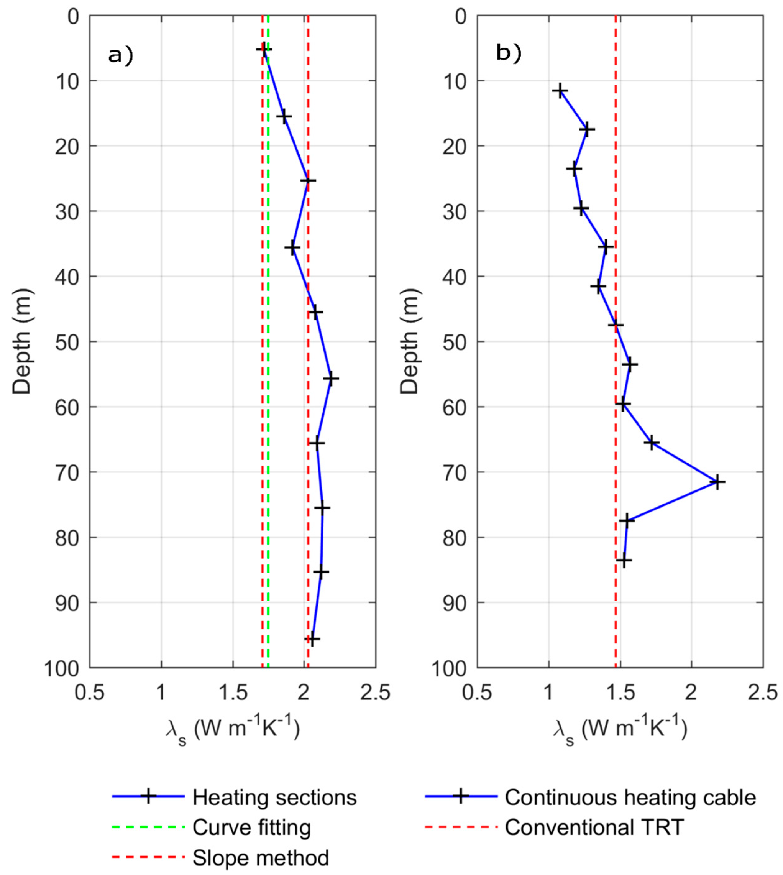
4.1. Thermal Conductivity Estimation

The analysis described below was based on submersible temperature measurements. A heat capacity of 2.3 MJ·m−3·K−1 associated with shales was assumed to compute the temperature increments and reproduce observations recorded for the first test in Québec City. The first 30 h of the recovery period was neglected and the analysis considered only the last 40 h to avoid the influence of the sensor location in the temperature measurement.
Adjustment between observed and computed temperature increments was achieved at the depth of each submersible temperature sensor tied to a heating section (Figure 7). However, to avoid repetition, only the curve matched at 45 m depth is provided as an example.
The first 20 h of the recovery period was neglected for the assessment of the thermal conductivity for the second test in Orléans. The temperature during the late recovery period was plotted as a function of the logarithmic time (Figure 8) and the slope of this line was used to determine the thermal conductivity at each measurement depth with submersible sensors according to Equation (8).
The estimated thermal conductivity in Québec City ranged 1.72–2.19 W·m−1·K−1, with an average value of 2.02 W·m−1·K−1 (Figure 9a). Minimal and maximal thermal conductivities of 1.71 and 2.03 W·m−1·K−1 were estimated in the conventional TRT with water circulation using the slope method and considering a constant heat injection rate. The maximal value was estimated during a TRT with a constant flow rate, and the minimal value during a second TRT in which the flow rate was reduced after 30 h of heat injection. A thermal conductivity of 1.75 W·m−1·K−1 was further obtained with analysis of the conventional TRT using the line source model with the superposition principle to consider variations in the heat injection rate [29,38]. The thermal conductivity points estimated with the heating cable section methodology differ between −25.30% and 1.70% from the bulk value estimated during the conventional TRT, using the line source model with a variable heat injection rate, while it is closer to the upper range of the slope analysis assuming constant heat injection rate.
The bulk thermal conductivity estimated with the conventional TRT in Orléans was 1.47 W·m−1·K−1 [39], while thermal conductivity points identified with the heating cable methodology varied from 1.08 to 2.18 W·m−1·K−1 with a mean value of 1.47 W·m−1·K−1. Differences varying from −48.30% to 26.53% were found when comparing the thermal conductivity profile with the bulk result of the conventional test. The maximal difference was found at 71.60 m depth, corresponding to the maximal thermal conductivity (Figure 9b).

4.2. Uncertainty Analysis

The absolute error of the measured parameters was determined from the accuracy associated with the measurement instruments (Table 2), except for the electrical resistance of the non-heating cable section, which was measured in the laboratory during previous work [40] and where the standard deviation of the measurements was used for the absolute error.
Measurement errors in Table 2 provided the basis to calculate combined errors in Table 3 to identify the accuracy of the heat injection rate (q) and the uncertainty of the analysis method, whether it is the finite line source equation (Z) or the slope (m′) with the infinite line source equation. The parameters Z and m were calculated using the data of each temperature sensor such that the values presented in Table 3 are the mean of all the sensors.
The uncertainty of the point thermal conductivity assessment estimated for each profile was calculated from the combined errors. An uncertainty varying from 0.27 to 0.33 W·m−1·K−1 was determined for the test with heating cable sections (Table 4) with a mean value of 0.31 W·m−1·K−1 (15.18%). An uncertainty varying from 0.02 to 0.05 W·m−1·K−1 was obtained for the continuous heating cable test (Table 5), with a mean value of 0.03 W·m−1·K−1 (2.14%).

4.3. Free Convection Assessment

The FO-DTS measurements enlarged for a heating section taken as an example indicate that the highest recorded temperature is located in the upper part of the heating sections (Figure 10). This observation combined with the temperature increments of about 2 °C away from the heating sections and highlighted in Figure 5 suggest the presence of free convection in the GHE pipe water during TRT with heating sections, even though perforated plastic disks were used to reduce convection.
The Rayleigh number was evaluated with temperature recorded in the pipe water for the heating section example from approximately 40 to 46 m depth (Figure 5 and Figure 10). The top of the system was fixed at 40.6 m, a depth at which the minimum temperature during the heat injection was recorded. The Rayleigh number calculation was done with temperature data recorded at 25, 95 and 121 h, representing the beginning and the end of the heat injection, and the recovery period, respectively. The highest Rayleigh number occurs at the end of the heat injection period near the location of the heating section and up to 1.5 m above. The maximal Rayleigh value is located at the upper part of the heating section, agreeing with the temperature peak (Figure 11).
The three critical lengths of 3, 6, and 9 m to calculate the critical Rayleigh number with Equation (27) were compared to the actual Rayleigh number. When defining Ht = 3 m, the Rayleighactual > Rayleighcritical for all the cases considered (28.5, 95, and 121 h), suggesting the presence of significant heat transfer by free convection in all the water column. Nevertheless, the recorded temperature between 41 and 43 m depth did not have an important variation and free convection at this depth was not expected. The choice of Ht = 3 m can be too small for the studied system.
In the second case, defining Ht = 6 m, Rayleighactual at the beginning of the heat injection (28.5 h) and during the recovery period (121 h) did not exceed the critical value. However, Rayleighactual > Rayleighcritical at the end of the heating period (95 h) for a portion of the heating section and up to 1.50 m above, suggesting the presence of free convection. The third case, considering Ht = 9 m, shows a critical Raleigh number that is always larger the than actual Rayleigh number, suggesting the absence of free convection. Defining Ht = 9 m can, however, overestimate Rayleigh’s critical value, since temperature increases far above from the heating section is a strong evidence of heat transfer due to free convection.
The effect of the perforated plastic disks to reduce free convection is difficult to evaluate. Nevertheless, the Rayleigh number reaches its maximal value at the top of the heating section (45 m) and decreases above heating sections where the perforated plastic disks were located. A similar effect occurs at the end of the heating section.
A similar analysis was done for the test with the continuous heating cable at 98.6, 234.6 and 404.6 h, corresponding to the beginning of the heating period, the end of the heating period, and the end of recovery period, respectively. The critical Rayleigh number was evaluated with a minimum critical height of 2 m. In this case, the critical Rayleigh number was not exceeded during any of the three selected times (Figure 12). A difference of approximately one order of magnitude was observed between the actual Rayleigh number and its critical value, showing that free convection is not a dominant heat transfer mechanism during the test with the continuous heating cable. The analysis was not repeated with higher critical length because it will result in higher critical Rayleigh number, increasing the difference with the actual Rayleigh number.

5. Discussion

The monitoring of temperature for the whole cable assemblies using FO-DTS allowed evaluating the temperature evolution beyond the submersible sensors to better understand the heat transfer phenomena occurring during both TRTs in addition to assessing thermal conductivity profiles of the ground. Thermal conductivity values are provided with error estimation for each case. In the case of the heating cable sections, it was particularly important to evaluate the temperature increases near the heating section extremities and along the non-heating sections. The additional temperature data provided by the FO-DTS allowed to identify significant temperature increases at the top of the heating sections and slight temperature increments at the middle of the non-heating sections, where temperature changes were not expected.

5.1. Thermal Conductivity Estimation

The subsurface thermal conductivity was evaluated using the finite and infinite line source solutions, to simulate conductive heat transfer at both tests with heating cable sections and a continuous heating cable. A thermal conductivity profile with a mean value of 2.02 ± 0.31 W·m−1·K−1 was estimated from the test with heating cable sections conducted in Quebec City, Canada. This value is 15.45% higher than the thermal conductivity evaluated during a conventional TRT made on the same GHE with water circulation analyzed with the infinite line source model and considering variations in the heat injection rate [29,38]. Analysis of a conventional TRT can, however, depends on the analysis method itself. The mean thermal conductivity estimated with the heating section TRT carried out in Quebec City differs by only 0.47% when compared to the maximum bulk thermal conductivity evaluated with the slope method for a conventional TRT performed in the same GHE [29,38]. A previous field test with heating cable sections reported by Raymond et al. [24] indicates a mean thermal conductivity 12% higher than that estimated with a conventional TRT. These results suggest that TRT with heating cable sections can slightly overestimate the ground thermal conductivity when compared to a conventional TRT. Free convection generated above the heating cable section can explain this difference since TRT analysis is made considering conductive heat transfer only. Free convection in a TRT using heating cable sections was identified by Raymond and Lamarche [23], through numerical simulation of the borehole temperature evolution during a TRT. The use of perforated plastic disks placed at the extremities of the heating section had been suggested to reduce the possible free convection. Nevertheless, the effect of natural convection was still identified during the full-scale test with heating cable sections, indicating that the four perforated plastic disks are not sufficient to totally control free convection during the heat injection period. A test with a reduced heat injection rate could be performed to evaluate if natural convection induced by the heating sections decreases.
The analysis of the Rayleigh number stability criteria for the GHE in Quebec City, made of a single U-pipe and drilled in sedimentary rocks, was conducted in a section of the GHE pipe considering half of a non-heating section (40.0–45.0 m) and a heating section (45.0–46.2 m) to have a temperature gradient increasing with depth as it is expected in analogous ground water well [28]. Considering the significant temperature increase above the heating section and the results of the Rayleigh number stability criterion with a critical height of 6 m, the presence of free convection is likely to be significant along the heating section and approximately 1.5 m above it.
A mean thermal conductivity of 1.47 ± 0.03 W·m−1·K−1 was estimated for the test with a continuous heating cable carried out in the GHE made of a double U-pipe drilled in limestone in Orléans, France. This value corresponds exactly to the bulk thermal conductivity estimated with the conventional TRT [39]. Previous comparison between TRT using continuous heating cable and a conventional TRT has not been made before. A constant initial temperature increase with depth, influenced by the natural geothermal gradient was observed before the TRT and seems to remain during the heat injection period with the continuous heating cable. Free convective heat transfer due to the geothermal gradient or caused by anthropogenic heat sources is possible since it has been observed in groundwater wells [28] and in the water column of open boreholes [41,42]. However, this weak convection mechanism can be neglected for TRT analysis, where heat conduction triggered upon heat injection is assumed more important than any natural convection. The actual Rayleigh number for the test performs with the continuous heating cable did not exceed the critical Rayleigh number evaluated between 18 m and 42 m depth, indicating that convective heat transfer can be neglected in this case. In future works, the thermal conductivity could be evaluated using the FO-DTS to allow an increase in the spatial resolution currently limited by the number of temperature sensors and to provide an additional independent estimation of the thermal conductivity.

5.2. Uncertainty Analysis

Uncertainty of TRT with heating cable sections conducted at a small scale was initially evaluated by Simon [27], which reported an accuracy of approximately 25% of the estimated thermal conductivity. A similar methodology adapted for the field test had been applied here. The highest uncertainty for the test is the error associated with the heat injection rate (δq = 6.07 W·m−1). The estimate of the electric resistance of the heating sections is the parameter with the most important uncertainly when calculating the heat injection rate. The uncertainty of the heat injection rate corresponds to 76–96% of the total test uncertainty. The remaining proportion of uncertainty corresponds to the error associated with the analytical model (δZ). The final test uncertainty ranged 14.6–16.4%, showing a reduction of approximately 10% compared to the uncertainly estimated during the laboratory tests performed in three 10 m wells [27]. The power injected underground for the laboratory tests was divided into three heating cable sections using a power switching supplies because three single heating section tests were carried out at the same time. The efficiency of this switch influenced the uncertainty of the heat injection rate, increasing the total uncertainly of the test. The electric current transmitted to the cable inducing the thermal power injected underground for the full-scale test presented in this study was controlled by a voltage regulator and measured using a power meter at the entry of the cable assembly, allowing to reduce the uncertainty associated to the evaluation of the heat injection rate. To adapt error calculation for conventional TRT to continuous heating cable TRT, both of which are using the slope analysis method, some modifications were introduced to the approach proposed by Witte [35]. The error of the heat injection rate and the slope of the regression of the temperature increments were calculated as a combination of errors for the continuous heating cable TRT. It was not necessary to calculate the average temperature, as in a conventional TRT, because the analysis was based on the temperature increments measured at the depth of each temperature sensor. The error associated with the heat injection rate only depended on the electric current intensity and the electric potential difference that are measured with accuracy in the field. Thus, the accuracy of the temperature sensors only influences the error attributed to the slope when plotting the temperature response.
The parameter with the highest uncertainty for the continuous heating cable TRT is the heat injection rate, with an error of 0.21 W·m−1, which corresponds to 99% of the total uncertainty. The remaining 1% corresponds to the uncertainty of the slope. The final uncertainty of the thermal conductivity profile was 2.14%, a lower value than the 5.10% estimated for a conventional TRT by Witte [35]. The accuracy of the heat injection rate appears to be the key factor, in any TRT method, that directly affects the uncertainty of the thermal conductivity estimate. Achieving an accurate assessment of the heat injection rate for TRTs with flowing water based on flow rate and temperature measurements tend to be more difficult than evaluating the heat injection rate transmitted through a continuous heating cable with potential difference and current intensity measurements. However, these measurements become complex for heating sections TRT, increasing the uncertainly associated with the analysis performed with the finite line source solution. This last analysis method with the finite line source solution requires assuming the heat capacity of the geological formation [23], adding an additional uncertainly to the analysis.

5.3. Comparison of TRT Methods

The assessment of thermal conductivity as a function of depth achieved using the heating cable methodology allows to define advantageous drilling conditions for the GHE according to the vertical ground thermal conductivity variations. The ground thermal conductivity inferred with a high spatial resolution, also obtained with TRTs coupled to FO-DTS, is valuable when detailed simulations of the GHE performance with several ground layers are considered.
Both heating cable sections and a continuous heating cable allowed reducing the power required to perform a TRT, as well as avoiding issues associated with water circulation, when compared to conventional tests (Table 6). The test error is reduced with a continuous heating cable compared to conventional TRT [43] and heating sections TRT [27], for which the estimation of the heat injection rate has most influence on the test error that is increasing when comparing the three methods (Table 6).
The time required to perform a TRT with a continuous heating cable and a low power source can be longer than TRT with heating sections [24,23] or a conventional TRT with FO-DTS. However, the equipment is left on site and there is no need for a follow-up, which reduces the time spend in the field and the cost of operations.
The temperature monitoring during the recovery period is necessary in all cases, when trying to infer the thermal conductivity at depth [24], making the test longer than the 50–80 h recommended for conventional heat injection TRTs [13] assessing the bulk thermal conductivity only. However, the estimation of the thermal conductivity based on the recovery temperature is more appropriate than using the heat injection period only [44]. The heat injection rate per unit length has to be considerably low with a continuous heating cable of approximately 100 m in length, resulting in an increase of the heat injection period to achieve a minimum temperature increase of at least 3 °C in the GHE pipe. However, the reduction of the test uncertainty and the simplified field manipulations make the continuous heating cable test a reliable alternative to perform TRT. In boreholes of more than 150 m, the increase of the cable weight can be a challenge to install and remove the cable that could be done with a winch. The test time could further be reduced with the improvement of the resolution of submersible temperature sensors that could detect smaller temperature perturbations to decrease the minimum temperature increase and, consequently, test time.

6. Conclusions

Thermal conductivity profiles and the errors associated were estimated at two different experimental sites using alternative heating cable methods to conduct the thermal response tests (TRT). The assessment of free convection in the standing water column suggested the presence of significant convection inside the pipe of the ground heat exchanger during the heat injection period when the heating cable sections were used. This analysis indicates that the perforated plastic disks installed at the interface between the heating and the non-heating sections do not remove all free convection during the heat injection period. However, the uncertainty range of the subsurface thermal conductivity estimated with heating section TRT was within the value inferred for a conventional TRT with water circulation. Considering the significant temperature increase observed above the heating section in the TRT carried out in Quebec City, the active heating length used to estimate the thermal conductivity can be revaluated. Further analysis is required to evaluate the ratio of conduction and convection heat transfer to adjust the test analysis methodology. Laboratory tests, comparing a standing water column with a column in which free convection is avoided using additives to make water become a gel, could be performed in future work to assess the temperature decrease caused by free convection movements. Convective heat transfer could additionally be taken into account for the analysis process through numerical simulations including free convective heat transfer mechanism.
The field tests performed, including the free convection and the uncertainty analysis, indicates that the TRT with the continuous heating cable has a better accuracy than the heating sections TRT. The assumption of dominant conductive heat transfer is valid when using the continuous heating cable and the total uncertainly of the test is lower than that obtained for both, the heating sections TRT and a conventional TRT with water circulation carried out under typical circumstances. The TRT with heating cable sections provides advantages to perform tests in deep boreholes (potentially more than 100 m), without increasing the heat injection rate and the power requirement. However, the analysis of the heating section TRT is limited by the effect of free convection that is not included in the analytical modeling approach. The limiting factor associated with the continuous heating cable TRT in deep boreholes is the electric resistance of the cable that increases with its length. The heat injection rate can be reduced maintaining a low power requirement, as shown in this study, but the use of high resolution temperature sensors to measure small temperature differences becomes necessary. TRT with a continuous heating cable and a low power source is a promising method and further tests could be carried out in boreholes of more than 100 m to verify the applicability of this methodology in ground heat exchangers commonly installed for ground-coupled heat pump systems.

Author Contributions

Conceptualization, M.I.V.M.; Data curation, M.I.V.M., M.P. and N.S.; Formal analysis, M.I.V.M.; Funding acquisition, J.R., M.P. and O.B.; Methodology, J.R. and D.B.; Project administration, J.R.; Resources, J.R., M.P. and O.B.; Supervision, J.R., D.B. and M.P.; Writing—original draft, M.I.V.M.; and Writing—review and editing, J.R., D.B., M.P., N.S., O.B. and L.L.

Acknowledgments

The Natural Sciences and Engineering Research Council of Canada and the Agence Nationale de la Recherche (ANR) in France are acknowledged for funding this research. This work is part of the ANR project EQUIPEX CRITEX (grant ANR-11-EQPX-0011), the ANR 13-SEED-0009 Stock en Socle project and the LIA France-Québec RESO “REssources et SOciétés” from which it has been supported. Nicolas Lavenant, who took part in the field experiment in Quebec City, is warmly acknowledged for his help and technical support. The Bureau de Recherches Géologiques et Minières in Orléans, France, is acknowledged for providing access to the experimental geothermal test facility in Orléans to conduct a part of this research. The International Geoscience Programme (IGCP), the United Nations Educational, Scientific and Cultural Organization (UNESCO), and the International Union of Geological Sciences (IUGS) are finally acknowledged since this work is part of the project “IGCP 636-Unifying international research forces to unlock and strengthen geothermal exploitation of the Americas and Europe”, currently funded by UNESCO and IUGS under the IGCP.

Conflicts of Interest

The authors declare no conflict of interest.

Nomenclature

(M L T t I) are used to denote units of mass, length, temperature, time and electric current, respectively
FoFourier’s number (-)
Ggravitational acceleration (L t-2)
gfinite heat source function (-)
hlength of heat source (L)
Hheight of the water column (L)
Ielectric current intensity (I)
mslope (-)
nnumber of observations (-)
qheat injection rate per unit length (M L t−3)
Relectric resistance (M L2 t-3 I−2)
rradius (L)
RaRayleigh number (-)
Serror of the estimate
ttime (t)
Ttemperature (T)
Uelectric potential difference (M L2 t-3 I−1)
Greek symbols
αthermal diffusivity (L2 t−1)
λthermal conductivity (M L T−1 t−3)
δuncertainty
σstandard deviation
νcinematic viscosity (L2 t−1)
subscripts
aaspect-ratio (-)
ccalculated
crcritical
hheating
nhnon-heating
mmeasured
offend of heat injection
ssubsurface
tcritical height
tottotal
0initial condition

References

  1. Marcotte, D.; Pasquier, P. On the estimation of thermal resistance in borehole thermal conductivity test. Renew. Energy 2008, 33, 2407–2415. [Google Scholar] [CrossRef]
  2. Zhang, C.; Guo, Z.; Liu, Y.; Cong, X.; Peng, D. A review on thermal response test of ground-coupled heat pump systems. Renew. Sustain. Energy Rev. 2014, 40, 851–867. [Google Scholar] [CrossRef]
  3. Mogensen, P. Fluid to duct wall heat transfer in duct system heat storages. In Proceedings of the International Conference on Subsurface Heat Storage in Theory and Practice, Stockholm, Sweden, 6–8 June 1983. [Google Scholar]
  4. Eklöf, C.; Gehlin, S. TED-a Mobile Equipment for Thermal Response Test: Testing and Evaluation. Master’s Thesis, Luleå University of Technology, Luleå, Sweden, 1996. [Google Scholar]
  5. Austin, W.A., III. Development of an In Situ System for Measuring Ground Thermal Properties. Master’s Thesis, Oklahoma State University, Stillwater, OK, USA, 1998. [Google Scholar]
  6. Gehlin, S. Thermal Response Test Method Development and Evaluation. Ph.D. Thesis, Luleå University of Techonology, Luleå, Sweden, 2002. [Google Scholar]
  7. Sanner, B.; Hellström, G.; Spitler, J.; Gehlin, S. More Than 15 years of Mobile Thermal Response Test—A Summary of Experiences and Prospects. Available online: https://hvac.okstate.edu/sites/default/files/pubs/papers/2013/03-Sanner_et_al_2013_EGC_TRT-overview.pdf (accessed on 3 May 2017).
  8. Spitler, J.D.; Gehlin, S. Thermal response testing for ground source heat pump systems—An historical review. Renew. Sustain. Energy Rev. 2015, 50, 1125–1137. [Google Scholar] [CrossRef]
  9. Gehlin, S. Thermal Response Test: In Situ Measurements of Thermal Properties in Hard Rock. Licentiate Dissertation, Luleå University of Technology, Luleå, Sweden, 1998. [Google Scholar]
  10. Raymond, J.; Therrien, R.; Gosselin, L. Borehole temperature evolution during thermal response tests. Geothermics 2011, 40, 69–78. [Google Scholar] [CrossRef]
  11. Carslaw, H.S. Introduction to the Mathematical Theory of the Conduction of Heat in Solids; Macmillan: London, UK, 1921. [Google Scholar]
  12. Ingersoll, L.R.; Plass, H.J. Theory of the ground heat pipe heat source for the heat pump. Trans. Am. Soc. Heat. Vent. Eng. 1948, 20, 119–122. [Google Scholar]
  13. Kavanaugh, S.P. Investigation of Methods for Determining Soil Formation Thermal Characteristics from Short Term Field Tests; ASHRAE: Atlanta, GA, USA, 2001. [Google Scholar]
  14. Sanner, B.; Hellström, G.; Spitler, J.; Gehlin, S. Thermal response test—Current status and world-wide application. In Proceedings of the World Geothermal Congress, Antalya, Turkey, 24–29 April 2005. [Google Scholar]
  15. Fujii, H.; Okubo, H.; Itoi, R. Thermal response tests using optical fiber thermometers. GRC Trans. 2006, 30, 545–551. [Google Scholar]
  16. Gehlin, S.; Hellström, G. Influence on thermal response test by groundwater flow in vertical fractures in hard rock. Renew. Energy 2003, 28, 2221–2238. [Google Scholar] [CrossRef]
  17. Gustafsson, A.M.; Westerlund, L. Heat extraction thermal response test in groundwater-filled borehole heat exchanger—Investigation of the borehole thermal resistance. Renew. Energy 2011, 36, 2388–2394. [Google Scholar] [CrossRef]
  18. Bense, V.F.; Read, T.; Bour, O.; Le Borgne, T.; Coleman, T.; Krause, S.; Chalari, A.; Mondanos, M.; Ciocca, F.; Selker, J.S. Distributed Temperature Sensing as a downhole tool in hydrogeology. Water Resour. Res. 2016, 52, 9259–9273. [Google Scholar] [CrossRef] [Green Version]
  19. Fujii, H.; Okubo, H.; Nishi, K.; Itoi, R.; Ohyama, K.; Shibata, K. An improved thermal response test for U-tube ground heat exchanger based on optical fiber thermometers. Geothermics 2009, 38, 399–406. [Google Scholar] [CrossRef]
  20. Beier, R.A.; Acuña, J.; Mogensen, P.; Palm, B. Vertical temperature profiles and borehole resistance in a U-tube borehole heat exchanger. Geothermics 2012, 44, 23–32. [Google Scholar] [CrossRef]
  21. Acuña, J.; Palm, B. Distributed thermal response tests on pipe-in-pipe borehole heat exchangers. Appl. Energy 2013, 109, 312–320. [Google Scholar] [CrossRef]
  22. Freifeld, B.M.; Finsterle, S.; Onstott, T.C.; Toole, P.; Pratt, L.M. Ground surface temperature reconstructions: Using in situ estimates for thermal conductivity acquired with a fiber-optic distributed thermal perturbation sensor. Geophys. Res. Lett. 2008, 35. [Google Scholar] [CrossRef] [Green Version]
  23. Raymond, J.; Lamarche, L. Development and numerical validation of a novel thermal response test with a low power source. Geothermics 2014, 51, 434–444. [Google Scholar] [CrossRef]
  24. Raymond, J.; Lamarche, L.; Malo, M. Field demonstration of a first thermal response test with a low power source. Appl. Energy 2015, 147, 30–39. [Google Scholar] [CrossRef]
  25. Raymond, J.; Robert, G.; Therrien, R.; Gosselin, L. A novel thermal response test using heating cables. In Proceedings of the World Geothermal Congress, Bali, Indonesia, 25–29 April 2010. [Google Scholar]
  26. Raymond, J. Colloquium 2016: Assessment of the subsurface thermal conductivity for geothermal applications. Can. Geotech. J. 2018, 55, 1209–1229. [Google Scholar] [CrossRef]
  27. Simon, F. Développement D’une Approche Nouvelle Pour Les Tests de Réponse Thermique en Géothermie. Master’s Thesis, École de technologie supérieure, Montréal, QC, Canada, 2016. [Google Scholar]
  28. Love, A.J.; Simmons, C.T.; Nield, D.A. Double-diffusive convection in groundwater wells. Water Resour. Res. 2007, 43. [Google Scholar] [CrossRef] [Green Version]
  29. Raymond, J.; Ballard, J.-M.; Koubikana Pambou, C.H. Field assessment of a ground heat exchanger performance with a reduced borehole diameter. In Proceedings of the 70th Canadian Geotechnical Conference and the 12th Joint CGS/IAH-CNC Groundwater Conference, Ottawa, ON, Canada, 1–4 October 2017. [Google Scholar]
  30. Philippe, M. Development and Experimental Validation of Vertical and Horizontal Ground Heat Exchangers for residential buildings heating. Ph.D. Thesis, École Nationale Supérieure des Mines de Paris, Paris, France, 2010. [Google Scholar]
  31. van de Giesen, N.; Steele-Dunne, S.C.; Jansen, J.; Hoes, O.; Hausner, M.B.; Tyler, S.; Selker, J. Double-ended calibration of fiber-optic raman spectra distributed temperature sensing data. Sensors 2012, 12, 5471–5485. [Google Scholar] [CrossRef] [PubMed]
  32. Lasdon, L.S.; Waren, A.D.; Jain, A.; Ratner, M. Design and testing of a generalized reduced gradient code for nonlinear programming. ACM Trans. Math. Softw. 1978, 4, 34–50. [Google Scholar] [CrossRef]
  33. Beck, A.E.; Anglin, F.M.; Sass, J.H. Analysis of heat flow data—In situ thermal conductivity measurements. Can. J. Earth Sci. 1971, 8, 1–19. [Google Scholar] [CrossRef]
  34. Pehme, P.E.; Greenhouse, J.P.; Parker, B.L. The active line source temperature logging technique and its application in fractured rock hydrogeology. J. Environ. Eng. Geophys. 2007, 12, 307–322. [Google Scholar] [CrossRef]
  35. Witte, H.J.L. Error analysis of thermal response tests. Appl. Energy 2013, 109, 302–311. [Google Scholar] [CrossRef]
  36. Evaluation of Measurement Data—Supplement 1 to the Guide to the Expression of Uncertainty in Measurement. Available online: https://www.bipm.org/utils/common/documents/jcgm/JCGM_101_2008_E.pdf (accessed on 9 September 2018).
  37. Ellison, S.; Williams, A. Eurachem/CITAC guide: Quantifying Uncertainty in Analytical Measurement. Available online: https://www.eurachem.org/images/stories/Guides/pdf/QUAM2012_P1.pdf (accessed on 12 July 2017).
  38. Ballard, J.M.; Koubikana, C.; Raymond, J. Développement des Tests de Réponse Thermique Automatisés et Vérification de la Performance des Forages Géothermiques d’un Diamètre de 4,5 Po. Internal Report R1601; Institut National de la Recherche Scientifique: Qubec City, QC, Canada, 2016. [Google Scholar]
  39. Maragna, C. Analyse D’un Test de Réponse Thermique; Internal Report; Division Géothermie, Bureau de Recherche Géologique et Minières de France: Orléans, France, 2014. [Google Scholar]
  40. Asselin, S. Manuel D’utilisation: Appareil de Lecture de Conductivité Thermique; Internal Report; Institut National de la Recherche Scientifique: Quebec City, QC, Canada, 2014. [Google Scholar]
  41. Klepikova, M.; Roques, C.; Loew, S.; Selker, J. Improved Characterization of Groundwater Flow in Heterogeneous Aquifers Using Granular Polyacrylamide (PAM) Gel as Temporary Grout. Water Resour. Res. 2018, 54, 1410–1419. [Google Scholar] [CrossRef]
  42. Berthold, S.; Resagk, C. Investigation of thermal convection in water columns using particle image velocimetry. Exp. Fluids 2012, 52, 1465–1474. [Google Scholar] [CrossRef]
  43. Witte, H.J.L.; van Gelder, G.; Spitler, J.D. In-situ thermal conductivity testing: A dutch perspective. ASHRAE Trans. 2002, 108, 263–272. [Google Scholar]
  44. Raymond, J.; Therrien, R.; Gosselin, L.; Lefebvre, R. A review of thermal response test analysis using pumping test concepts. Ground Water 2011, 49, 932–945. [Google Scholar] [CrossRef] [PubMed]
Figure 1. Stratigraphic description of the borehole located in: (a) Quebec City (modified from Raymond et al. [29]); and (b) Orléans (modified from Philippe [30]).
Energies 11 03059 g001
Figure 2. Apparatus for TRT with: (a) heating cable sections; and (b) a continuous heating cable (modified from Raymond [26]).
Energies 11 03059 g002
Figure 3. Junction box for TRT with a heating cable.
Energies 11 03059 g003
Figure 4. Temperature evolution during the three steps of the TRT in Quebec City with heating cable sections.
Energies 11 03059 g004
Figure 5. Observed temperature at the middle of a non-heating section (40 m) and at the top (45 m) and the middle (45.5 m) of a heating section.
Energies 11 03059 g005
Figure 6. Temperature evolution during the three steps of the TRT in Orléans with a continuous heating cable.
Energies 11 03059 g006
Figure 7. Observed and computed temperature increments (Equation (1)) during the recovery period for the submersible sensor located at 45 m depth for the test with heating cable sections.
Energies 11 03059 g007
Figure 8. Observed temperatures during the recovery period for the submersible sensor located at 53.6 m depth for the test with a continuous heating cable.
Energies 11 03059 g008
Figure 9. Point subsurface thermal conductivity (crosses) obtained with the (a) heating cable sections in Québec City and (b) the continuous heating cable in Orléans. The results are compared to the bulk values provided by the conventional TRT with water circulation (green and red dashed lines).
Energies 11 03059 g009
Figure 10. Temperature distribution during the TRT around a typical heating section at 45–46 m depth.
Energies 11 03059 g010
Figure 11. Verification of the Rayleigh number stability criterion considering different critical lengths Ht to calculate the critical Rayleigh number (dashed lines) for the test with heating cable sections.
Energies 11 03059 g011
Figure 12. Verification of the Rayleigh number stability criterion for the test with a continuous heating cable.
Energies 11 03059 g012
Table 1. Experimental condition and configuration of TRT.
ParameterQuebec CityOrléans
Heating cable typeHeating sectionContinuous heating cable
Test analysis methodFinite line sourceInfinite line source
Borehole configurationSingle U-pipeDouble U-pipe
TRT start date31 August 20163 July 2017
TRT start time11:20:0013:00:00
TRT end date7 September 20162 August 2017
TRT end time12:11:0010:00:00
Borehole depth (m)150100
Heating cable length (m)10095
Borehole diameter (mm)114180
Pipe diameter (mm)32.0026.20
Duration of undisturbed temperature monitoring (h)26.00100.00
Heat injection period (h)73.00135.70
Thermal recovery period (h)70.00481.30
Total test duration (h)169.00717.00
Initial temperature (°C)8.2013.10
Heat injection rate (W·m−1)42.509.90
Temperature sensors vertical distance (m)106
Table 2. Error associated to measured parameters.
Parameter Measured Repeatedly during the TestAbsolute ErrorRelative Error (%)Reference Value-Quebec CityReference Value-Orléans
Temperature T (°C)0.10
Electric power P (W)0.020.002985.13940.45
Electric current intensity I (A)0.020.178.718.99
Electric potential difference U (V)0.020.01113.12104.70
Parameter measured once and separately
Length of the heating cable H (m)0.010.01-95.00
Length of the heating section Lh (m)0.010.811.24-
Electrical resistance per unit length of the non-heating section Rnh (Ω·m−1)0.00020.500.04-
Table 3. Combined errors.
Continuous Heating CableAbsolute ErrorRelative Error (%)Reference Value
Heat injection rate q (W·m−1) 0.212.129.91
Slope m′ (-)0.0010.230.55
Heating Cable SectionAbsolute ErrorRelative Error (%)Reference Value
Total electrical resistance of the cable assembly Rtot (Ω)0.120.9412.99
Electrical resistance of the heating cable sections Rh (Ω)0.1314.260.90
Heat injection rate q (W·m−1) 6.0714.2942.50
Analytical model Z (-)1.065.0021.14
Table 4. Uncertainly of the point thermal conductivity assessment for the heating cable sections test in Québec City.
Depth (m)Thermal Conductivity (W·m−1·K−1)Absolute Error δk (W·m−1·K−1)Relative error (%)
5.31.720.2715.61
15.51.860.3116.38
25.42.030.3014.85
35.61.910.2915.02
45.52.070.3014.62
55.72.190.3314.95
65.62.080.3215.44
75.52.120.3315.31
85.42.120.3214.88
95.62.060.3014.73
Average2.020.3115.18
Table 5. Uncertainly of the point thermal conductivity assessment for the test with a continuous heating cable in Orléans.
Depth (m)Thermal Conductivity (W·m−1·K−1)Absolute Error δk (W·m−1·K−1)Relative Error (%)
11.61.080.022.13
17.61.270.032.13
23.61.180.032.13
29.61.230.032.13
35.61.40.032.13
41.61.350.032.13
47.61.470.032.14
53.61.570.032.14
59.61.520.032.13
65.61.720.042.14
71.62.180.052.15
77.61.550.032.13
83.61.530.032.14
Average1.470.032.14
Table 6. Comparison of TRT methods for thermal conductivity profile assessment.
ParameterContinuous Heating CableHeating Cable SectionsConventional with FO-DTS
Power requirementLowLowHigh
Test time+++++++
Equipment complexity++++++
Cost$$$$$$
Measured parametersT0, λsT0, λsT0, λs, Rb
Surface disturbancesNoNoYes
Analysis methodInfinite line source solutionFinite line source solutionInfinite line source solution

