An Optimal Burn-In Policy for Cellular Phone Lithium-Ion Batteries Using a Feature Selection Strategy and Relevance Vector Machine

Abstract

The early detection of defective lithium-ion batteries in cellular phones is critical due to the rapid increase in popularity and mass production of cellular phones. It is essential for manufacturers to design an optimal burn-in policy to differentiate between normal and weak batteries in short cycles prior to shipping them to the marketplace. A novel approach to determine the optimal burn-in policy using a feature selection strategy and relevance vector machine (RVM) is proposed. The sequential floating forward search (SFFS) is used as the feature selection method to find an optimal feature subset from the entire sequence of the batteries’ quality characteristics while preserving the original variables. Given the selected feature subset, the RVM is applied to classify batteries into two groups and simultaneously obtain the posterior probabilities. To achieve better discrimination performance with less risk, a new characteristic is extracted from the discharge profile. Subsequently, an optimization cost model is developed by introducing a classification instability penalty to ensure the stability of the optimal number of burn-in cycles. A case study utilizing cellular phone lithium-ion batteries randomly selected from manufactured lots is presented to illustrate the proposed methodology. Furthermore, we conduct a comparison with the cumulative degradation (CD) method and non-cumulative degradation (NCD) method based on the Wiener process. The results show that our proposed burn-in test method performs better than comparable methods.

1. Introduction

Lithium-ion batteries are commonly used in cellular phones due to their high energy density [1,2]. As a result of the current extensive use of lithium-ion batteries for cellular phones, difficulties arise to ensure the high quality of each lithium-ion battery before it is used in a phone. Moreover, as the use of smartphones is increasing extensively, lithium-ion batteries have become increasingly important for the user experience and market competitiveness of cellular phones. As a critical component in cellular phones, the performance of lithium-ion batteries plays an important role in ensuring the security and reliability of the entire system [3,4]. Therefore, before batteries are shipped to the marketplace, it is required that the battery quality be evaluated so that weak batteries do not affect the relationship between suppliers and customers and the risk of recalling cellular phones is minimized. The cycle life, which is related to battery life and is obtained from a degradation test [5], is one of the main characteristics that should be monitored but the evaluation of the cycle life is extremely costly and time-consuming. On that account, it is important to evaluate the quality of the battery as soon as possible after manufacturing. Due to market demand, it is critical for manufacturers to design an optimal burn-in policy to detect weak batteries before shipping them to the marketplace.

Burn-in tests are used for determining if a unit operates normally or is weak before the product reaches the consumers; these tests are applied to products to eliminate initial failures or weak items [6]. A traditional assessment of a product’s lifetime is based on failure-time data. However, in many cases, it is difficult to collect such failure data under normal operating conditions. For that reason, accelerated degradation tests (ADTs) have been used for reliability analyses by increasing the level of the variables, such as the vibration amplitude, temperature, corrosive media, load, voltage, and pressure [7,8]. However, for highly reliable products, ADTs provide little additional information because very few failures occur during the test. Therefore, if there exists a quality characteristic (QC) whose degradation over time can be related to reliability, then the products’ lifetime can be estimated based on the degradation model [9]. If a weak item degrades faster than a normal one, this item can be identified through a burn-in test. In a degradation-based burn-in test, all items are subject to the testing environment for a certain duration. If this unit’s QC degradation exceeds a burn-in cut-off level, then the unit is rejected and is not shipped to market. Otherwise, it will be accepted. A demonstration of a degradation-based burn-in test with simulation data is shown in Figure 1. The green lines represent the degradation paths of weak items which exceed the cut-off level and are unacceptable whereas the blue lines represent the degradation paths of normal items which indicate acceptable values and are accepted. Moreover, the cut-off level is much lower than the failure threshold so that the degradation-based burn-in test is able to identify a weak item much sooner than it fails.

One of the earliest attempts of degradation-based burn-in policies was proposed by Tseng and Tang [10]. The authors used a diffusion process to describe the degradation path of LED lamps. This model was further extended by Tseng et al. [11] and Tseng and Peng [12] based on variants of the Wiener process. Wang et al. [13] developed a linear Wiener-process-based model with adaptive drift to characterize the degradation trajectories. In order to model nonlinear degradation, the linear Wiener process with adaptive drift was extended to a nonlinear Wiener process with adaptive drift [14,15]. In addition, degradation models can also be developed based on other stochastic models, such as the gamma process [16] and inverse Gaussian process [17]. However, a major disadvantage of the procedure is that it only uses current degradation data and ignores any information given by the entire sequence of observations. To compensate for this, Tseng and Peng [12] proposed an integrated Wiener process to model the cumulative degradation path. Although it made use of the entire sequence of observations, it has a large computational cost due to the use of the integral of the degradation path, which is inconvenient in practical use. To address this problem, Peng [18] and Chen et al. [19] used a linear discriminant analysis (LDA) to design classification rules for making full use of the data. Furthermore, the degradation data are a sequence of real numbers representing the values of variables over time, including two-dimensional information, the time, and the value corresponding to the time. To this point, feature extraction methods such as the LDA are not suitable for this situation because they alter the original representation of the variables. In contrast, feature selection techniques that preserve the original semantics of the variables and merely select a subset of them have an advantage over data with two-dimensional information.

Feature selection techniques are an essential step prior to classification for making use of data, lest some redundant and meaningless sequences may result in increased computational costs and influence the classifier performance. When a feature selection process is completed, the next step is to select a good classifier. To this point, Park et al. [20] presented a dual-feature functional SVM approach that uses the first and second derivatives of the degradation profiles for the early detection of faulty batteries. Fisher et al. [21] used an SVM and automatic feature selection to perform anomaly detection in passive seismic data of earth dams and levees. SVMs have been used in a variety of classification applications, for example, Ma et al. [22], Ebrahimi et al. [23], Jaramillo et al. [24], and Li et al. [25]. Nevertheless, the outputs of an SVM represent decisions rather than posterior probabilities. Therefore, in this study, a relevance vector machine (RVM) and sequential floating forward search (SFFS) are applied to treat the aforementioned classification problem. Because the RVM is a non-linear probability model [26] and a Bayesian sparse kernel technique, which provides posterior probabilities, it shares many properties with an SVM.

In this paper, we propose a burn-in policy for phone batteries to ensure that defective batteries are found at a specific time, namely, the burn-in time, which is optimized considering appropriate criteria. There are two criteria for determining the optimal burn-in time; (1) the first is the expected cost; this has been addressed in the studies by Tsai et al. [27], Ye et al. [28,29], Liu et al. [30], and Zhai et al. [31]; (2) The second criterion is the products’ performance, such as the mean residual lifetime and the mean number of failures. Models related to this have been described in the studies by Bebbington et al. [32], Cha and Finkelstein [33], Ye et al. [34], and Yu and Peng [35]. Shafiee et al. [6] pointed out that the existing cost optimization models have focused on the first criterion by minimizing a cost function. In this paper, we aim to differentiate batteries into normal and weak items in short cycles before the batteries are shipped to a marketplace. To ensure that the burn-in time is stable and reliable in case of random values based on minimizing the current cost model, an optimization model to minimize the total expected cost is developed. Our objective function includes the expected burn-in cost and a penalty for the classification instability to seek a trade-off between the performance of the classifier and the burn-in time. A penalty for the classification instability ensures the stability of an optimal number of burn-in cycles in case of random values.

A novel approach is proposed to find the optimal burn-in time in this study. First, the RVM and SFFS methods are used for the classification to make full use the entire sequence of observations. The floating search method is presented to select an optimal feature subset among the entire sequence of observations because this subset is rich in discriminatory information for the classification design and the redundant and meaningless features that increase the computational burden and influence the classifier performance have been removed. In addition, to achieve a better discrimination of the two groups in the early cycles with less risk, a new characteristic is extracted from the voltage and current during the discharge profile. Subsequently, an improved optimization cost model that introduces a penalty for the classification instability is utilized to determine the battery’s optimal number of burn-in tests by minimizing the proposed cost function. A case study is presented to illustrate the proposed methodology and determine the classification performance of different QC combinations. Furthermore, we conduct a comparison with the non-cumulative degradation (NCD) method, cumulative degradation (CD) method, and our proposed method. The results show that our proposed method for burn-in test provides better performance than comparable methods.

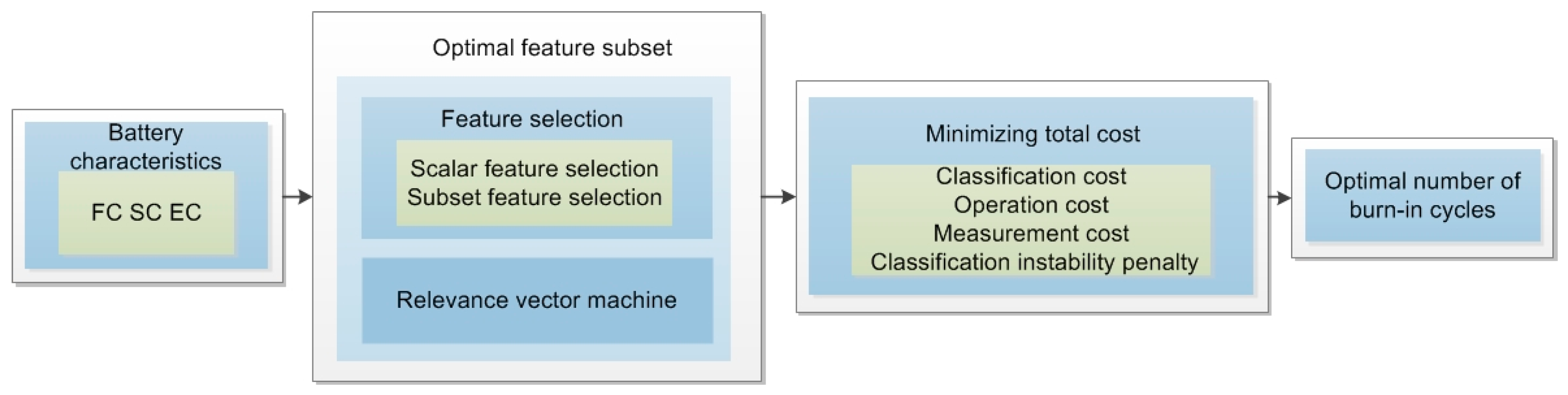
2. Framework of Optimal Burn-In Policy Design

Components designated for high-reliability applications are often subject to “burn-in” to weed out the weak items. For a traditional burn-in test during battery manufacturing, each battery goes through cycles until it meets a fixed threshold, such as the normal threshold value of 80% of the initial capacity. Thus, the traditional burn-in test is extremely costly and time-consuming. Instead of conducting long burn-in tests, this study focuses on the design of an optimal burn-in policy to differentiate between normal and weak batteries in short cycles prior to shipping them to a marketplace.

To intuitively illustrate the procedure of the optimal burn-in test design, a block diagram is shown in Figure 2. According to the analysis of real data, the capacity and a new characteristic equivalent internal resistance (EIR) are regarded as the main QCs presenting the degradation of batteries. The first derivatives and the second derivatives of the remaining capacity (FC and SC) and the EIR (EC) as battery characteristics represent the classier input, and they are then expressed as a vector. Prior to the classification, feature selection techniques are an essential step prior to classification for making use of the vector. Furthermore, the RVM combined with feature selection provides an optimal feature subset by minimizing the classification cost. Given a defined cost model, the optimal number of burn-in cycles is determined by minimizing the total cost. In the end, A case study utilizing cellular phones lithium-ion batteries randomly selected from manufactured lots is presented to illustrate the proposed methodology.

3. Battery Characteristics Selection

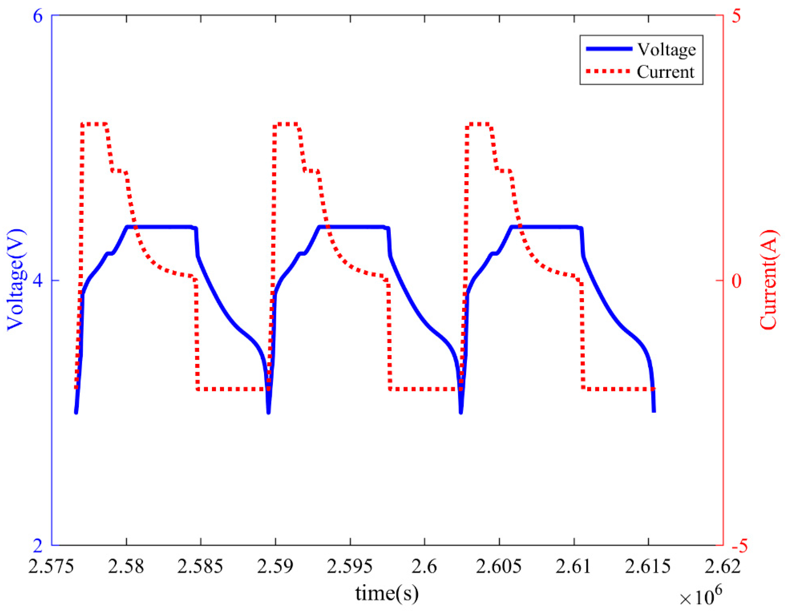
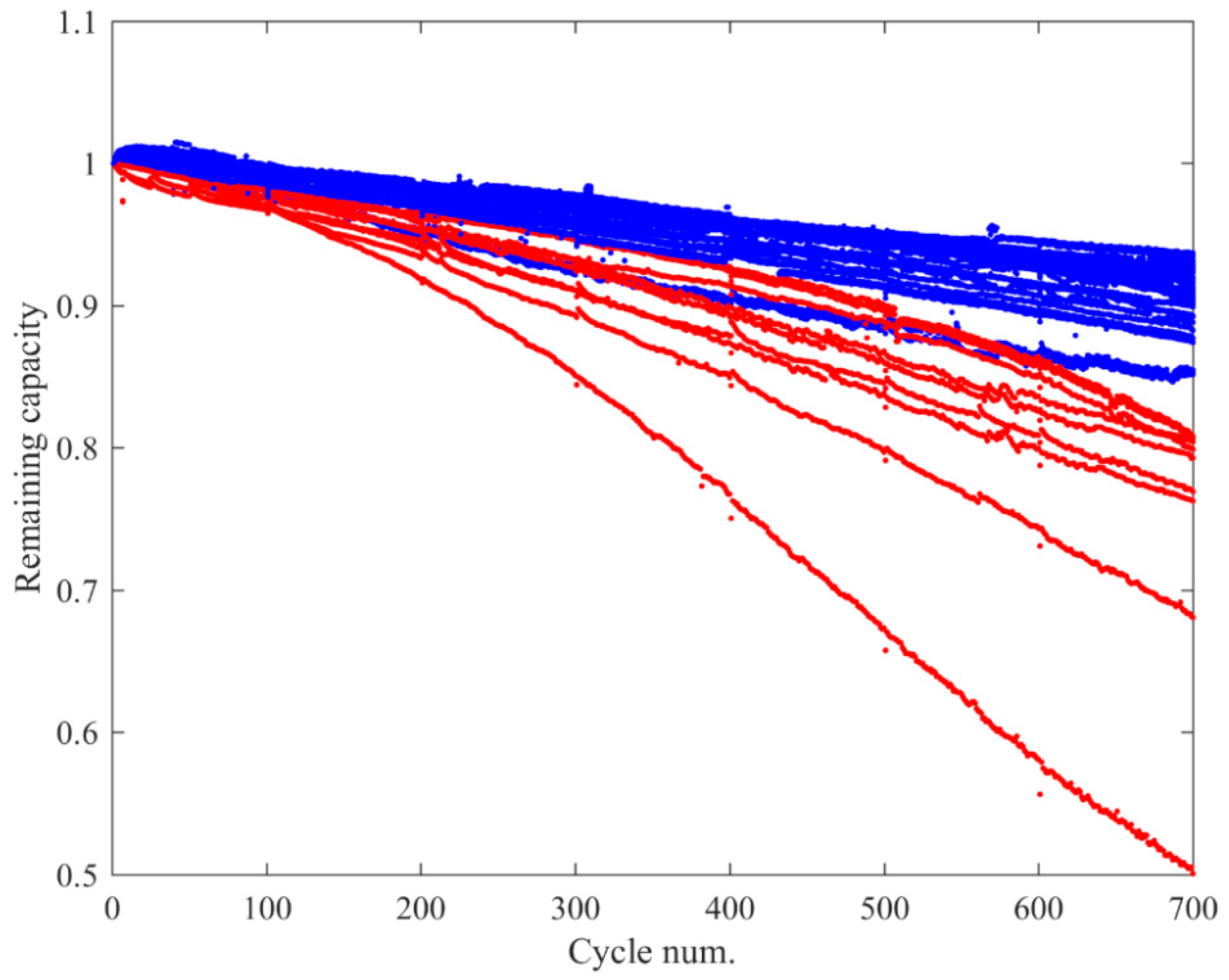
3.1. Data Description

In order to present our proposed optimal burn-in policy for cellular phone lithium-ion batteries, data consisting of randomly selected 45 sample profiles (33 profiles of normal samples and 12 profiles of weak samples) during a burn-in test were obtained from manufactured lots over several months. An experiment consisting of repeated iteration of a series of charging and discharging profiles followed by a full recharge to 4.4 V and cycling of these samples is conducted at a constant ambient temperature of 25 °C. In the experiment, 45 samples were aged with the same profile under equal conditions. The cut-off voltage and maximum charge voltage were 3 V and 4.4 V respectively.

The batteries were continuously operated by repeatedly charging them to 4.4 V and then discharging them to 3.0 V under a fixed load, as shown in Figure 3. During the charging cycles, the batteries were first charged at about 3.0 A (constant current) until they reached 4.4 V, at which time the charging was switched to a constant voltage mode and charging continued until the charging current fell below 0.01 A. Aside from the capacity, the basic characteristic of a lithium-ion battery that can be related to reliability was measured at every cycle. The batteries were continuously operated under a fixed load of up to 700 cycles. Figure 4 shows the remaining capacity degradation paths of 45 cells of lithium-ion batteries of cellular phones up to 700 cycles. Note that the true labels (normal items and weak items) of these batteries are determined by the remaining capacity in the 700th cycle. The 33 blue lines represent the remaining capacity degradation paths of normal items while the 12 red lines represent the normal items’ paths. It is evident that the capacity of the battery decreases as the number of cycles increases. Furthermore, the remaining capacity of the weak items degrades faster than that of the normal items. This provides an opportunity to differentiate between the normal and weak items as soon as possible. However, the weak and normal units start to diverge when the number of cycles increases to about 200. Similarly, it is riskier to determine the conditions of the batteries in the early cycles than to use a traditional burn-in test. Therefore, it is necessary to develop an efficient procedure to discriminate normal batteries from weak items in short cycles.

3.2. Battery Characteristics

The basic characteristic of a lithium-ion battery that can be related to reliability is its capacity, which is defined as the number of hours that a battery can provide a current at the discharge rate of the nominal voltage. As seen in Figure 4, it is clear that the capacity of the battery decreases as the number of cycles increases. In addition, the decline in the remaining capacity has a nonlinear function; the capacity degrades slowly during the initial cycles whereas it degrades sharply in the later cycles. This nonlinear property of capacity degradation increases the difficulty of determining the condition of the batteries in the early cycles. However, as mentioned earlier, the remaining capacity of the weak items degrades faster than that of the normal items. This provides an opportunity to differentiate between the normal and weak items as soon as possible. The boxplot in Figure 5 shows the distribution of the remaining capacity of the normal items (33 cells) and weak items (12 cells) for several fixed cycles. There are significant differences in the remaining capacity between the normal items and the weak items, except for the cycles before No. 30. Therefore, the remaining capacity is a useful characteristic. Note that there are some outliers owing to measurement errors or operations that do not cover a full cycle.

In order to provide a better separation of the two groups in the early cycles with less risk, a new characteristic is introduced in this study and is determined by analyzing the voltage and current in the discharge profile, as seen in Figure 6. A full cycle consists of two profiles, i.e., the charging profile and the discharging profile. In the charging profile, the voltage is charged to 4.4 V and remains in this state until the current decreases to 0.7 A at $t_1$. Then when the current drops to zero at $t_2$, the state of a battery switches to the discharging profile and simultaneously the voltage drops to $U_R$ due to the internal resistance of the battery. The characteristic $U_R$ is the voltage loss of the internal resistance and is called the equivalent internal resistance (EIR) hereafter. As shown in Figure 6, the voltage loss is very small during the charging and discharging process. However, since the EIR has been normalized, it represents a remarkable change in the battery’s cycle life, as shown in Figure 7 (normal items: blue lines and weak items: red lines). The new normalized characteristic EIR of 45 lithium-ion batteries decays as the cycle proceeds, reflecting the battery deterioration. In addition, As a whole, the EIR degradation paths of the weak items (red lines) decay faster than the normal items (blue lines). The EIR box plots of the normal and weak batteries are shown in Figure 8. Except for the early cycles, the two groups exhibit considerable differences in the distribution of the EIR. Therefore, it is concluded that the EIR is suitable to serve as an index of the battery’s degradation.

Based on these results, the remaining capacity and EIR are used as criteria for battery classification. We use the first derivatives and the second derivatives of the remaining capacity (FC and SC) and the EIR (EC) as battery characteristics. A cubic spline is used for interpolation to calculate the first derivatives and the second derivatives. This method avoids the sudden changes between given points and provides numerical stability in the direct computation.

4. Classifier Design with Feature Selection Strategy

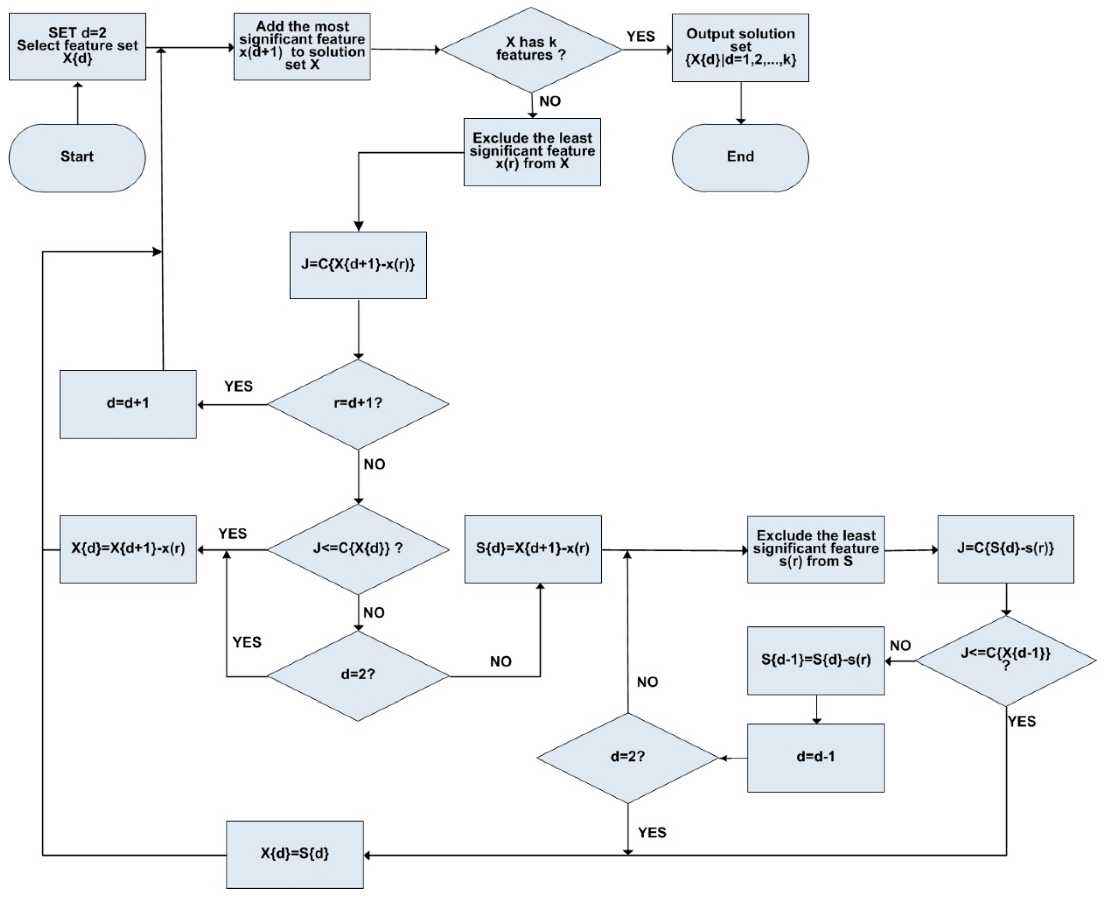
4.1. Feature Selection

Based on the results, the FC, SC, and EC are regarded as the battery degradation characteristics; they represent the classier input and are then ordered in a vector. However, prior to classification, feature selection is an essential step for making use of the vector. Feature selection is aimed at finding the optimal subset of features from a larger pool of available features. It aims to select those that are rich in discriminatory information for the classification design because features that are redundant and meaningless result in increased computational burden and influence the classifier performance. The SFFS method presented by Pudil et al. [36] is an effective feature selection method. Ashok and Aruna [37] determined that the SFFS method had better performance than the mutual information (IM), sequential forward search (SFS), and random subset feature selection (RSFS) methods. Moreover, in this study, the feature selection consists of two steps: scalar feature selection and subset feature selection. Scalar feature selection is used to eliminate redundant and meaningless features and subsequently, we use the features selected in the scalar feature selection step in the SFFS to obtain the optimal feature combination. The use of the scalar feature selection greatly reduces the computational complexity because a large number of features mixed with irrelevant features will result in an exponential increase in computations with an increasing number of features [38].

Considering the case of the training data set $\{{(Q_i,Z_i)}_{i=1,2,3,\dots ,n}\}$, $Q_i=\left\{q_i\left(1\right),q_i\left(1\right),\dots ,q_i\left(t\right)\right\}$ for the observed number of cycles t and a binary class index $Z_i\in \left\{0,1\right\}$, we search for the optimal number of features $d^{\ast }$ for the given number of cycles t. First, we perform the scalar feature selection, which uses the Fisher Discrimination Ratio (FDR) to rank m features in descending order {$f_1,f_2,\dots ,f_m$}. Subsequently, the correlation between the features to sort the features [39] is determined. Let $f_1$ be the index of the optimal feature $i_1$, then the second feature $i_l\left(l\ge 2\right)$ can be obtained by:

$$i_{l=}\{\begin{array}{c}\underset{j}{\max }\{a_1{C}_j-a_2\left|{\rho }_{i_1,j}\right|\},j\ne i_1,l=2;\\ \underset{j}{\max }\{a_1{C}_j-\frac{a_2}{l-1}{\displaystyle {\displaystyle \sum }_{r=1}^{l-1}}\left|{\rho }_{i_r,j}\right|\},j\ne i_r,r=1,2,\dots ,l-1,l=3,4,\dots ,m\end{array}$$

(1)

where $C_j$ is the FDR criterion of feature j, ${\rho }_{i_1,j}$ is the cross-correlation between feature $i_1$ and feature j, and $a_1$, $a_2$ are coefficients.

Then we use the top $k$ features as the input features for the SFFS, which is one of the most effective feature selection techniques. The method begins with an empty subset and then features are added or excluded based on the criterion function until the desired number of features is obtained. Scatter matrices are among the most popular performance measures for feature subset selection due to their rich physical meaning. Here, the SFFS method is employed to determine the optimal feature subset by maximizing the $J_3$ criteria function. The $J_3$ criteria function is defined as:

$$J_3=trace\left\{S_w^{-1}{S}_b\right\}$$

(2)

where $S_w$ is the within-class scatter matrix and $S_b$ is the between-class scatter matrix. The detailed procedure for the SFFS method is shown below Figure 9:

• Input: A set of $Q_i=\left\{x_j\right|2\le j\le k\}$, d is the desired number of features, $C\left\{d\right\}$ is the criterion function with the feature subset $X\left\{d\right\}$;
• Output: the optimal feature subsets $\left\{X\left\{d\right\}\right|2\le d\le k\}$
  Initialization: d = 2, using sequential forward selection, select the feature subset $X\left\{d\right\}$.

4.2. Classifier Design

The RVM is a Bayesian sparse kernel technique and provides posterior probabilities; it shares many properties with the SVM. For a binary classification, the RVM model is expressed as:

$$y\left(\mathit{x},\mathit{w}\right)=f\left({\mathit{w}}^T\mathbf{\varphi }\left(\mathit{x}\right)\right)$$

(3)

where f(•) is a logistic sigmoid function, $\mathbf{\varphi }\left(\mathit{x}\right)$ denotes a feature-space transformation, and $\mathit{w}$ is the parameter vector. Here we use the Laplace approximation [40] for this model. Beginning with initializing a hyperparameter vector $\mathbf{\alpha }$, we then create a Gaussian approximation of the posterior distribution and maximize an approximation log marginal likelihood to update the value of $\mathbf{\alpha }$; this process repeats until convergence or the maximum number of iterations is reached. The steps of the procedure are as follows:

• Given a fixed value of $\mathbf{\alpha }$, the posterior distribution over $\mathit{w}$ is obtained by maximizing

  $$lnp\left(\mathit{w}|\mathit{z},\mathbf{\alpha }\right)={\displaystyle \sum }_{i=1}^N\left\{t_{i}ln\left(y_i\right)+\left(1-t_i\right)ln\left(1-y_i\right)\right\}-\frac{1}{2}{\mathit{w}}^T\mathit{A}\mathit{w}$$

  (4)

  where A = diag($\mathbf{\alpha }$) and $\mathit{z}$ is a target value vector. The iterative reweighted least squares (IRLS) method [41] is applied to solve this problem. Then the mean and covariance of the Gaussian approximation is expressed as:

  $${\mathit{w}}^{\ast }={\mathit{A}}^{-1}{\mathit{\Psi }}^{\mathit{T}}\left(\mathit{z}-\mathit{y}\right)$$

  (5)

  $$\Sigma ={({\mathit{\Psi }}^{\mathit{T}}\mathit{B}\mathit{\Psi }+\mathit{A})}^{-1}$$

  (6)

  where $\mathit{\Psi }$ is the design matrix with elements ${\mathit{\Psi }}_{ni}={\mathbf{\varphi }}_i\left({\mathit{x}}_n\right)$; B is an N × N diagonal matrix with $b_{ii}=y_i\left(1-y_i\right)$.
• Suppose $\widehat{\mathit{z}}=\mathit{\Psi }{\mathit{w}}^{\ast }+{\mathit{B}}^{-1}\left(\mathit{z}-\mathit{y}\right)$, then the approximate log marginal likelihood in the form is obtained by:

  $$lnp\left(\mathit{z}|\mathbf{\alpha }\right)=-\frac{1}{2}\left\{Nln\left(2\pi \right)+ln\left|\mathit{C}\right|\right\}+{\widehat{\mathit{z}}}^T{\mathit{C}}^{-1}\widehat{\mathit{z}}$$

  (7)

  where $\mathit{C}=\mathit{B}+{\mathit{\Psi }}^T\mathit{A}\mathit{\Psi }$. Then $\mathbf{\alpha }$ can be updated by:

  $${\alpha }_i^{new}=\frac{{\gamma }^i}{{(w_i^{\ast })}^2}$$

  (8)

  where ${\gamma }^i=1-{\alpha }_i{\Sigma }_{ii}$.
• The previous two steps are repeated until convergence or a maximum number of iterations is reached.
• Then the output $y$ is calculated by $y\left(\mathit{x},\mathit{w}\right)=f\left({\mathit{w}}^T\mathbf{\varphi }\left(\mathit{x}\right)\right)$; assuming that the threshold of the posterior probabilities is $\xi$, then $z=1\mathrm{if}y\ge \xi \mathrm{and}0\mathrm{otherwise}.$

Given a subset of k features, the RVM is applied to distinguish the normal and weak batteries. Due to the limited data set of the capacity degradation sample, the leave-one-out (LOO) method is used to determine the optimal $d^{\ast }$ feature subset. Considering that the desired number of features is given by d, the SFFS is used to find the optimal d feature subset $\left\{X_d\right|2\le d\le k\}$ with $J_3$ criteria. Therefore, for the observed number of cycles t, the $d^{\ast }$ feature subset is calculated as:

$$d^{\ast }=\underset{2\le d\le k}{\min }MC\left(t,d\right)$$

(9)

$$MC\left(t,d\right)=\frac{1}{n}({{\displaystyle \sum }}_{i=1}^n\left(1-g_i\right)\left(c_1{h}_i+c_2\left(1-h_i\right)\right)+{\displaystyle \sum }_{i=1}^n{g}_i{F}_i)$$

(10)

$$F_i=-(c_1{h}_i\log \left(p_i\right)+c_2\left(1-h_i\right)\log \left(p_i\right))$$

(11)

where $MC\left(t,d\right)$ denotes the per unit cost of the classification; $c_1$ is the cost of the Type I error (the normal unit is classified as a weak unit); $c_2$ is the cost of the Type II error (the weak unit is classified as a normal unit); n is the total number of samples; $g_i=1$ if the RVM returns the correct output of sample i and 0 otherwise; $h_i=1$ if the target output of sample i is 1 and 0 otherwise; $p_i$ is the posterior probability of (${\mathit{z}}_i=1$). The classification cost expressed in Equation (10) is based on the definition of the misclassification cost used in many studies and in addition, a new type of a classification cost $F(•)$ inspired by a likelihood function, first presented in [42], is proposed. The classification cost consists of two kinds of cost; one is the misclassification cost when the RVM classifier returns the wrong output, and the other is the penalty cost according to the posterior probability when the classifier obtains the correct output. The second cost aims to obtain higher posterior probabilities of P($z_i=1$) when the target output is 1 and lower posterior probabilities of P($z_i=1$) when the target output is 0. At the number of test cycle t, the average error rate is given by:

$$erro{r}_t=\frac{1}{n}{\displaystyle \sum }_{i=1}^{n}I[\Theta \left(X\left\{t,d\right\},z_i\right]$$

(12)

where $\Theta (X\left\{t,d\right\}$ is the RVM classifier with the feature subset X{$t,d$}; $I\left[b_1,b_2\right]=1$ if $b_1=b_2$ and 0 otherwise.

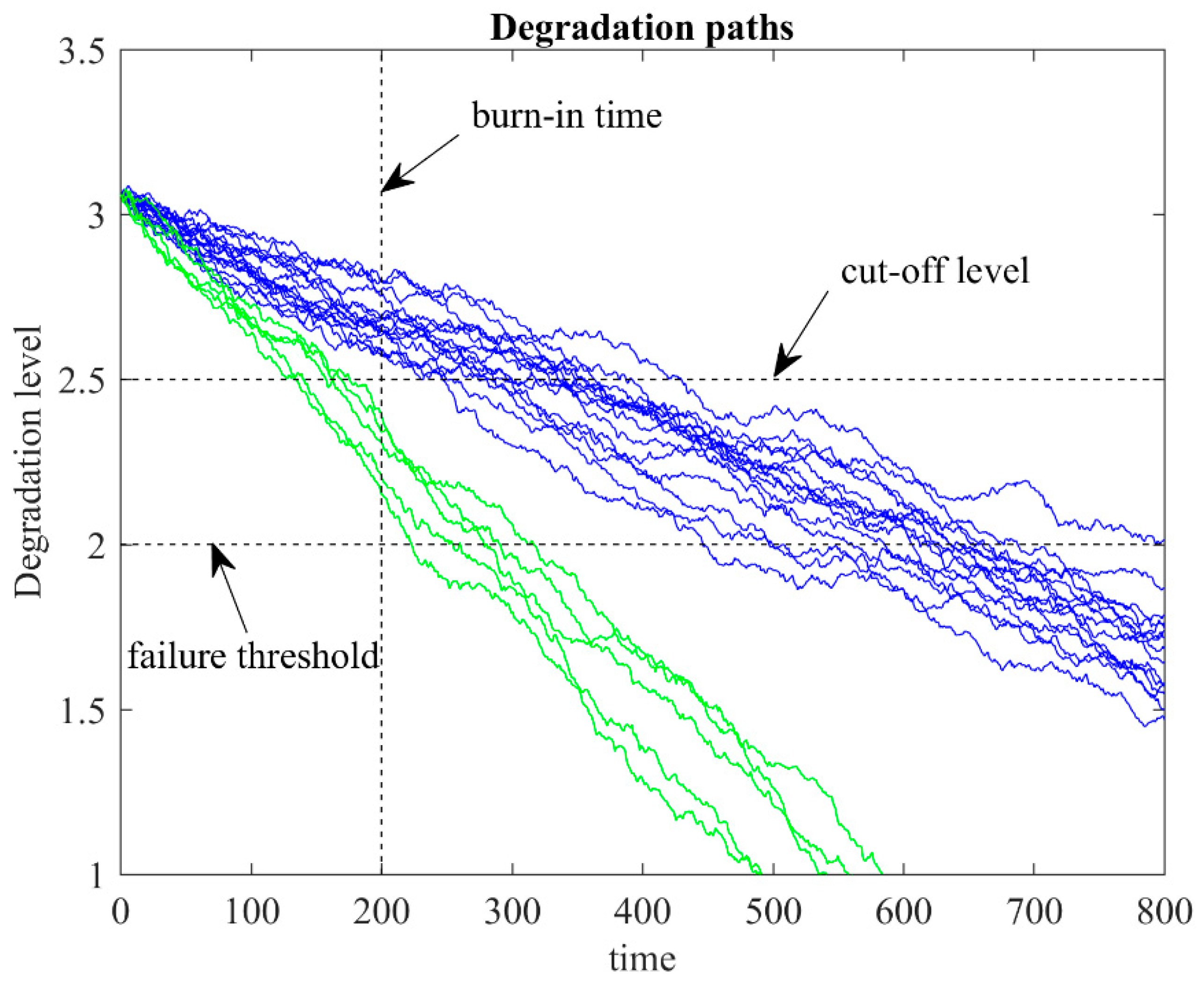
5. Optimal Number of Burn-In Cycles

A cost model is used to determine the optimal number of burn-in cycles. The cost model can be assessed in terms of the cost of the classification, the operation cost, the measurement cost, and the penalty of classification instability. A trade-off between the performance of the classifier and the number of burn-in cycles is obtained by the cost model. The developed cost model is expressed as:

$$TC\left(t,d^{\ast }\right)=MC\left(t,d^{\ast }\right)+C_{ope}\times t\times l+C_{mea}\times t+PC\left(t,d^{\ast }\right)$$

(13)

where $C_{ope}$ and $C_{mea}$ denote the per unit cost of operating a cycle life test per unit of time and the cost of measuring the data of a unit, respectively. l is the average discharge time. $PC\left(t,d^{\ast }\right)$ is the function of the penalty of classification instability given the test cycle $t$. Assuming that $PC\left(t,d^{\ast }\right)$ is an exponential function, $PC\left(t,d^{\ast }\right)$ can be calculated as:

$$PC\left(t,d^{\ast }\right)=C_{pen}\times \exp \left(S\left(t\right)\times n\right),t>p$$

(14)

$$S\left(t\right)=\sqrt{\frac{1}{2p}{\displaystyle \sum }_{i=t-p}^{t+p}{(err{o}_i-\mu )}^2},t>p$$

(15)

where $C_{pen}$ is the cost penalty of the classification instability per unit; p is the window size; $\mu$ is the mean of the average classification error rate between the test cycle ($t-p$) and ($t+p$). Given the window size p, $S\left(t\right)$ denotes the standard deviation of the average classification error rate of the test cycle ($t-p$) to ($t+p$). The penalty of classification instability is introduced to avoid random values and to ensure the reliability of the selected optimal number of burn-in cycles.

Finally, the optimal number of burn-in cycles $t^{\ast }$ can be directly obtained by enumerating $t\in \mathit{t}$ to minimize the total cost TC function:

$$t^{\ast }=\underset{t\in \mathit{t}}{min}TC\left(t,d^{\ast }\right)$$

(16)

6. Results and Discussion

6.1. Results

To illustrate our proposed procedure, we use 45 sample profiles (33 profiles of normal samples and 12 profiles of weak samples) randomly selected from manufactured lots. As shown in Figure 1, the weak units degrade faster than the normal units. If these weak batteries are not removed, not only does it affect the customer’s goodwill but it also affects then warranty and increases the replacement costs. The proposed optimal burn-in policy for the burn-in test is thus necessary to eliminate the weak units. To demonstrate our proposed method, the following cost profile is used:

• The cost of a Type I error $c_1=\$100$
• The cost of a Type II error $c_2=\$150$
• Operational cost $C_{ope}=\$0.02/\mathrm{h}$
• Measurement cost $C_{mea}=\$0.1$
• Classification instability penalty cost $C_{pen}=\$5$

To determine the effect of a combination of features, the changes in the selected optimal feature subsets using the RVM and the SFFS method are observed. With regard to this, we should note that the characteristics including the FC, SC, and EC are regarded as the classifier input, which is ordered in a vector of features. For example,

Table 1. Selected feature subsets.

Cycle Num.	Selected Feature Subsets (d = 10)
	FC	SC	EC
10	[2, 3, 6, 9]	[11, 12, 13]	[21, 23, 25]
20	[4, 7, 10]	[32, 35]	[42, 43, 46, 54, 57]
30	[10, 13, 21, 23]	[43, 48, 50, 53]	[60, 61]
40	[4, 10, 13, 21]	[53, 58, 63, 73]	[83, 86]
50	[10, 13]	[54, 73, 92]	[101, 122, 125, 132, 147]
60	[10, 13]	[64, 83, 102]	[121, 142, 145, 152, 167]

shows each selected feature subset (d = 10) from the 10th cycle to the 60th cycle, given a vector of features. The results demonstrate that each feature does work in different periods but has different weights. As seen in Table 1, the selected features of the FC may be relatively more successful in the earlier cycles than the later cycles. In contrast, half of the features belonging to the EC are selected in the later cycles, such as the 50th cycle and 60th cycle. This implies that the three selected characteristics (FC, SC, and EC) are rich in discriminatory information for the classification design.

Figure 10 shows the error rates of different combinations of battery characteristics for discriminating between normal and weak batteries using the RVM and the SFFS method. The error rate exhibits a monotonic function although there are some fluctuations. The third combination of characteristics has better classification performance than the second combination of characteristics, indicating that the proposed new characteristic EC is more effective for classification than the SC. Furthermore, our proposed combination of characteristics (FC, SC, and EC) is the optimal combination. Note that the proposed method with the combination still has tolerable error rates, even for the 20th cycle.

The selection of battery characteristics is a key issue in implementing our proposed method. Furthermore, the developed cost model is applied to determine the optimal number of burn-in cycles. Given the aforementioned cost profile, the optimal number of burn-in cycles is 35, and $T{C}^{\ast }=22.11\$$. Figure 11 shows the total classification cost versus the cycle number. The results show that in our proposed burn-in policy, the cost of the burn-in can be decreased significantly. Although the optimal number of burn-in cycles is 35, the error rate is still low at 0.044. This represents a good trade-off between the classifier performance and the number of burn-in cycles.

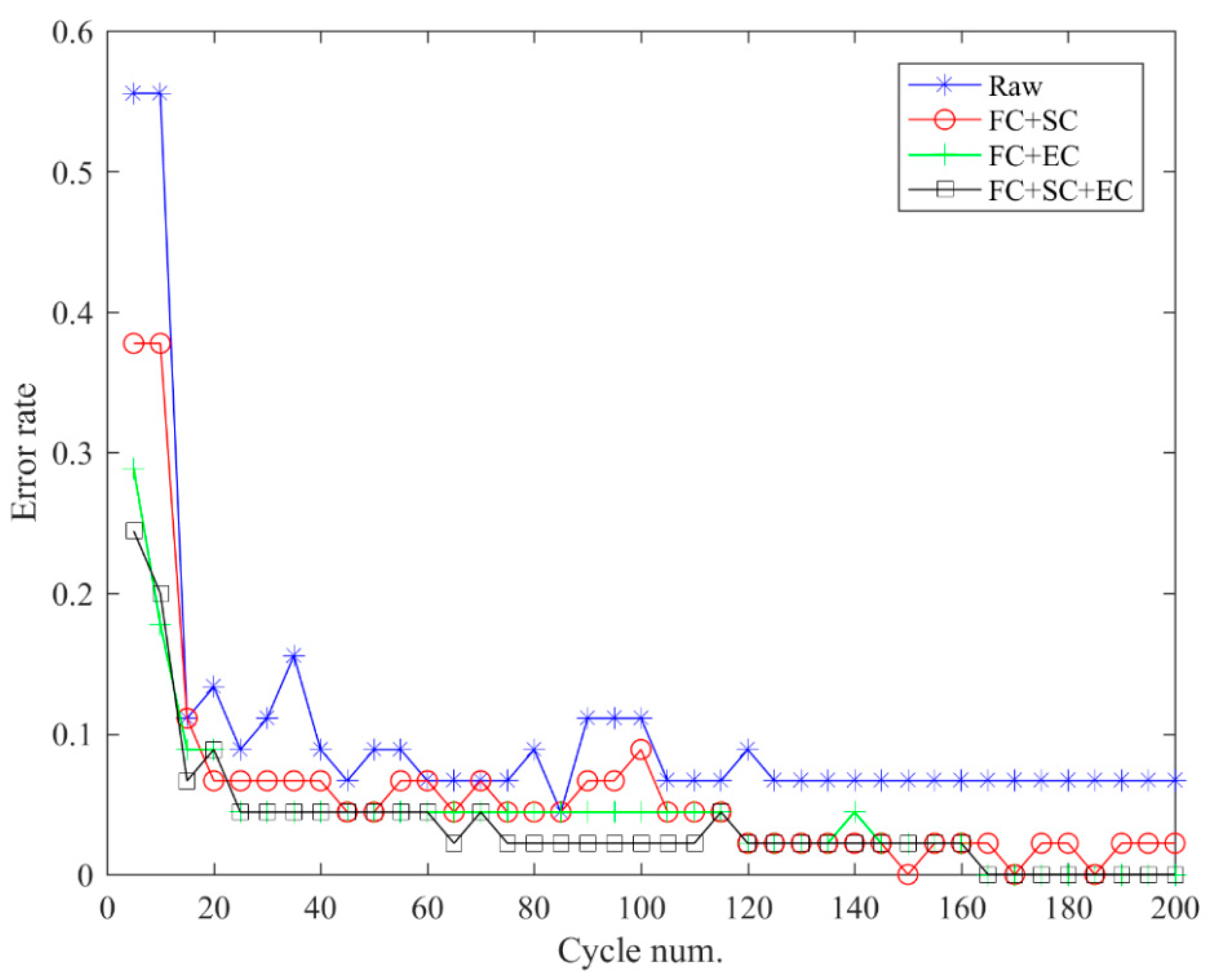
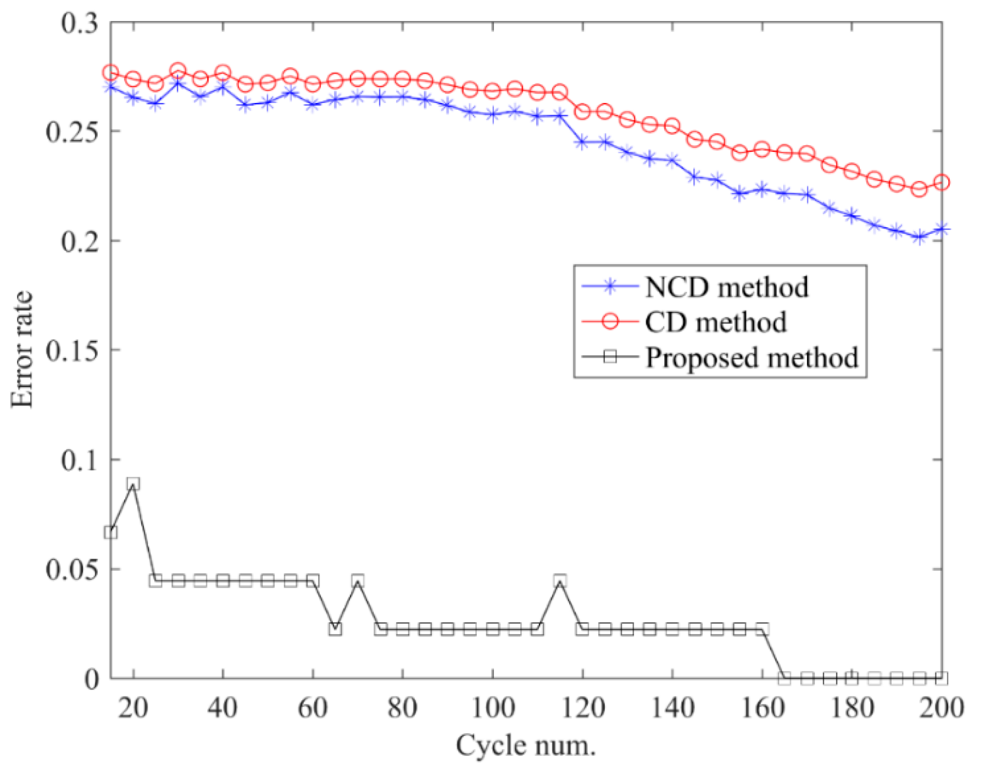
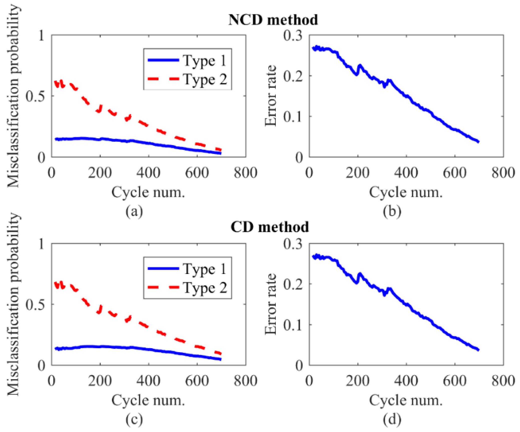
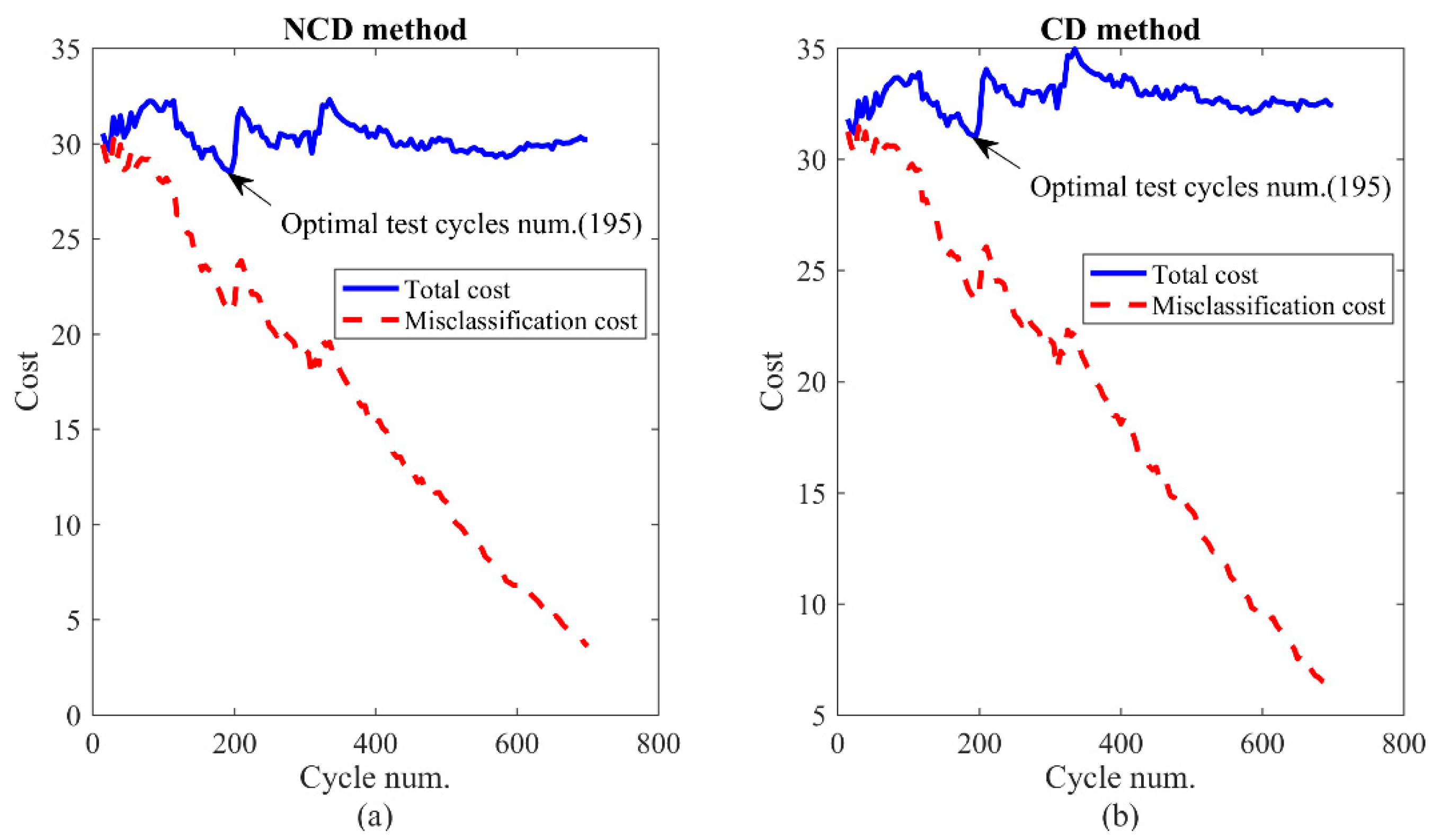
6.2. Comparison with Other Methods

In this section, a comparison between our proposed method and other typical methods used for a burn-in test is conducted to illustrate the advantage of our proposed methodology; we use the following criteria:

(a)

The error rate of the classification

(b)

The optimal number of burn-in cycles

Commonly used methods are the CD method proposed by Tseng et al. [8] and the NCD method proposed by Tseng and Peng [7]. The degradation model is based on the Wiener process of the NCD and CD methods and other details are shown in

Table 2. Comparison of the proposed method with the NCD and CD methods.

	NCD Method	CD Method	Proposed Method
Model	$L\left(t\right)=\{\begin{array}{c}{\Lambda }_1\left(t\right)+\sigma B\left(t\right),fornormalitems\\ {\Lambda }_2\left(t\right)+\sigma B\left(t\right),forweakitems\end{array}$	${{\displaystyle \int }}_0^{t}L\left(t\right)=\{\begin{array}{c}{{\displaystyle \int }}_0^t{\Lambda }_1\left(s\right)ds+\sigma {{\displaystyle \int }}_0^{t}B\left(s\right)ds,fornormalitems\\ {{\displaystyle \int }}_0^t{\Lambda }_2\left(s\right)ds+\sigma {{\displaystyle \int }}_0^{t}B\left(s\right)ds,forweakitems\end{array}$	$y\left(\mathit{x},\mathit{w}\right)=f\left({\mathit{w}}^T\mathbf{\varphi }\left(\mathit{x}\right)\right)$
Error rate	$error={\alpha }_1\left(1-p\right)+{\beta }_{1}p$	$error={\alpha }_2\left(1-p\right)+{\beta }_{2}p$	$error=\frac{1}{n}{\displaystyle {\displaystyle \sum }_{i=1}^n}I[\Theta \left(X\left\{t,d\right\},z_i\right]$
Misclassification cost	$MC\left(\xi \left(t\right),t\right)=\left(1-p\right)c_1\alpha +p\beta$		$\begin{array}{c}MC\left(t,d\right)=\frac{1}{n}({\displaystyle {{\displaystyle \sum }}_{i=1}^n}\left(1-g_i\right)(c_1{h}_i\\ +c_2\left(1-h_i\right))+{\displaystyle {\displaystyle \sum }_{i=1}^n}{g}_i{F}_i))\end{array}$
Optimal cut-off level	$\begin{array}{c}{\xi }_1\left(t\right)={\Lambda }_2\left(t\right)+\sqrt{{\sigma }^{2}t}(\frac{{\Delta }_1\left(t\right)}{2}\\ +\frac{ln\left(c_{2}p/\left(c_1\left(1-p\right)\right)\right)}{{\Delta }_1\left(t\right)})\end{array}$	$\begin{array}{c}{\xi }_2\left(t\right)={{\displaystyle \int }}_0^t{\Lambda }_2\left(s\right)ds+\sqrt{2{\sigma }^2{{\displaystyle \int }}_0^t\left(t-s\right)sds}(\frac{{\Delta }_2\left(t\right)}{2}\\ +\frac{ln\left(c_{2}p/\left(c_1\left(1-p\right)\right)\right)}{{\Delta }_2(t)})\end{array}$	$\xi$is determined as requested
Total cost	$TC(t)=MC(\xi (t),t)+C_{ope}\times t\times l+C_{mea}\times t$		$TC(t,d^{\ast })=MC(\mathrm{t},d^{\ast })+C_{ope}\times \mathrm{t}\times l+C_{mea}\times \mathrm{t}+PC(\mathrm{t},d^{\ast })$
Optimal test cycle num.	$t^{\ast }=minTC(t)$

where, $\Lambda (t)=\eta t$, $\eta$ is the drift parameter, $\sigma$ is the variance coefficient, and B(t) is the standard Brownian motion; p: proportion of the weak items in n unit; ${\Delta }_1=\frac{{\Lambda }_1(t)-{\Lambda }_2(t)}{\sqrt{{\sigma }^{2}t}},{\Delta }_2=\frac{{{\displaystyle \int }}_0^t{\Lambda }_1(s)ds-{{\displaystyle \int }}_0^t{\Lambda }_2(s)ds}{\sqrt{2{\sigma }^2{{\displaystyle \int }}_0^t(t-s)sds}}$; Type I error: $\alpha$; Type II error: $\beta$; ${\alpha }_1=\Phi (\frac{{\xi }_1(t)-{\Lambda }_1(t)}{\sqrt{{\sigma }^{2}t}})$, ${\beta }_1=1-\Phi (\frac{{\xi }_1(t)-{\Lambda }_2(t)}{\sqrt{{\sigma }^{2}t}})$, ${\alpha }_2=\Phi (\frac{{\xi }_2(t)-{{\displaystyle \int }}_0^t{\Lambda }_1(s)ds}{\sqrt{2{\sigma }^2{{\displaystyle \int }}_0^t(t-s)sds}})$, ${\beta }_2=1-\Phi (\frac{{\xi }_2(t)-{{\displaystyle \int }}_0^t{\Lambda }_2(s)ds}{\sqrt{2{\sigma }^2{{\displaystyle \int }}_0^t(t-s)sds}})$.

. The Wiener process describes the degradation path of the capacity. As observed in Figure 12, these results demonstrate that our proposed method of using the RVM and SFFS outperforms the commonly used classification methods. As shown in Figure 1, the weak units degrade faster than the normal units, providing an opportunity to differentiate them. However, the capacity degradation curves are very close to each other in the early cycles so that it is difficult to differentiate the units by a univariate degradation model with only one QC. In contrast, we use two QCs for a better discrimination of the batteries; one of them is extracted from the voltage and current during the discharge profile. Given the improved selection of the batteries’ QCs, we use the RVM and SFFS for the classification. In this approach, features are selected that are rich in discriminatory information for the classification and make full use of the entire sequence of the batteries’ QCs. In addition, the RVM is a Bayesian sparse kernel technique and provides posterior probabilities that ensure higher classification accuracy and better generalization ability. Thus, it performs better than the typical methods. Since in NCD and CD methods, they always need to obtain the misclassification probability to calculate the misclassification cost, the misclassification probability is provided in Figure 13a,c. And the error rate is also obtained in Figure 13b,d, which has been described in Figure 12.

Furthermore, the cost versus cycle number of NDC and CD methods is shown in Figure 14a,b respectively. As seen from Figure 14, the optimal number of burn-in cycles in these methods are 195, which is higher than for our proposed method. Besides, in the 195th cycle, both error rates are about 0.202, which is higher than 0.044 obtained by the proposed method. The comparison of the three methods verifies our method’s effectiveness. As mentioned earlier, the typical methods result in poor performance when the degradation paths are close to each other in the earlier cycles. In addition, the weak and normal units start to diverge when the number of cycles increases to about 200. At this point, the typical methods are not very effective for reducing the cost of the burn-in test.

7. Conclusions

In this paper, we have proposed an optimal burn-in policy to differentiate batteries into normal and weak units in short cycles before shipping the batteries to a marketplace. The combination of the RVM and SFFS algorithms results in excellent performance regarding the early detection of weak batteries. The hybrid method makes full use the entire sequence of the observation of batteries and ensures higher classification accuracy and better generalization ability. Instead of a univariate degradation model with only one QC, two QCs are proposed for a better discrimination of the batteries. One of them is the EC extracted from the discharge profile and, to some extent, it also enhances the classifier performance although the degradation curves of the two groups are very similar in the early cycles. In addition, a cost model is developed and includes a penalty for the classification instability that ensures the stability of an optimal number of burn-in cycles. The results show that the cost of the burn-in can be decreased significantly using our proposed burn-in policy. Although the optimal number of burn-in cycles is 35, the error rate is still low at 0.044. Furthermore, we compare the NCD and CD methods with our proposed method. The results show that our proposed method for the burn-in test performs better than the typical methods.

In future studies, we plan to expand this research. The degradation paths and measurement errors require further investigation. The measurement error should be considered in a classification method because it impacts the classification accuracy and decision making. Additionally, the quality loss is a factor worth exploring. Therefore, the classifier design and the development of cost models will be further investigated.

References

1. Mankowski, P.J.; Kanevsky, J.; Bakirtzian, P.; Cugno, S. Cellular phone collateral damage: A review of burns associated with lithium battery powered mobile devices. Burns 2016, 42, 61–64. [Google Scholar] [CrossRef] [PubMed]
2. Yu, J.; Liang, S.; Tang, D.; Liu, H. Remaining Discharge Time Prognostics of Lithium-Ion Batteries Using Dirichlet Process Mixture Model and Particle Filtering Method. IEEE Trans. Instrum. Meas. 2017, 66, 2317–2328. [Google Scholar] [CrossRef]
3. Yu, J.; Mo, B.; Tang, D.; Yang, J.; Wan, J.; Liu, J. Indirect State-of-Health Estimation for Lithium-Ion Batteries under Randomized Use. Energies 2017, 10, 2012. [Google Scholar] [CrossRef]
4. Patil, M.; Panchal, S.; Kim, N.; Lee, M.-Y. Cooling Performance Characteristics of 20 Ah Lithium-Ion Pouch Cell with Cold Plates along Both Surfaces. Energies 2018, 11, 2550. [Google Scholar] [CrossRef]
5. Panchal, S.; McGrory, J.; Kong, J.; Fraser, R.; Fowler, M.; Dincer, I.; Agelin-Chaab, M. Cycling degradation testing and analysis of a LiFePO4 battery at actual conditions. Int. J. Energy Res. 2017, 41, 2565–2575. [Google Scholar] [CrossRef]
6. Shafiee, M.; Chukova, S.; Yun, W.Y. Optimal burn-in and warranty for a product with post-warranty failure penalty. Int. J. Adv. Manuf. Technol. 2013, 70, 297–307. [Google Scholar] [CrossRef]
7. Shiau, J.J.H.; Lin, H.H. Analyzing accelerated degradation data by nonparametric regression. IEEE Trans. Reliab. 1999, 48, 149–158. [Google Scholar] [CrossRef]
8. Rohner, M.; Kerber, A.; Kerber, M. Voltage Acceleration of TBD and Its Correlation to Post Breakdown Conductivity of N- and P-Channel MOSFETs. In Proceedings of the 2006 IEEE International Reliability Physics Symposium Proceedings, San Jose, CA, USA, 26–30 March 2006; pp. 76–81. [Google Scholar]
9. Ye, Z.S.; Xie, M. Stochastic modelling and analysis of degradation for highly reliable products. Appl. Stoch. Models Bus. Ind. 2015, 31, 16–32. [Google Scholar] [CrossRef]
10. Tseng, S.T.; Tang, J. Optimal burn-in time for highly reliable products. Int. J. Ind. Eng. 2001, 8, 329–338. [Google Scholar]
11. Tseng, S.T.; Tang, J.; Ku, I.H. Determination of burn-in parameters and residual life for highly reliable products. Nav. Res. Logist. 2003, 50, 1–14. [Google Scholar] [CrossRef]
12. Tseng, S.T.; Peng, C.Y. Optimal burn-in policy by using an integrated Wiener process. IIE Trans. 2004, 36, 1161–1170. [Google Scholar] [CrossRef]
13. Wang, W.; Carr, M.; Xu, W.; Kobbacy, K. A model for residual life prediction based on Brownian motion with an adaptive drift. Microelectron. Reliab. 2011, 51, 285–293. [Google Scholar] [CrossRef]
14. Huang, Z.; Xu, Z.; Wang, W.; Sun, Y. Remaining Useful Life Prediction for a Nonlinear Heterogeneous Wiener Process Model with an Adaptive Drift. IEEE Trans. Reliab. 2015, 64, 687–700. [Google Scholar] [CrossRef]
15. Wang, D.; Tsui, K.L. Brownian motion with adaptive drift for remaining useful life prediction: Revisited. Mech. Syst. Signal Process. 2018, 99, 691–701. [Google Scholar] [CrossRef]
16. Tsai, C.; Tseng, S.; Balakrishnan, N. Optimal Burn-In Policy for Highly Reliable Products Using Gamma Degradation Process. IEEE Trans. Reliab. 2011, 60, 234–245. [Google Scholar] [CrossRef]
17. Zhang, M.; Ye, Z.; Xie, M. Optimal Burn-in Policy for Highly Reliable Products Using Inverse Gaussian Degradation Process. In Proceedings of the Engineering Asset Management–Systems, Professional Practices and Certification, Hong Kong, China, 30 October–1 November 2013; pp. 1003–1011. [Google Scholar]
18. Peng, C.Y. Optimal Classification Policy and Comparisons for Highly Reliable Products. Indian J. Stat. 2015, 77, 321–358. [Google Scholar] [CrossRef]
19. Chen, Z.; Xia, T.; Pan, E. Optimal multi-level classification and preventive maintenance policy for highly reliable products. Int. J. Prod. Res. 2016, 55, 2232–2250. [Google Scholar] [CrossRef]
20. Park, J.I.; Baek, S.H.; Jeong, M.K.; Bae, S.J. Dual Features Functional Support Vector Machines for Fault Detection of Rechargeable Batteries. IEEE Trans. Syst. Man Cybern. Part C Appl. Rev. 2009, 39, 480–485. [Google Scholar] [CrossRef]
21. Fisher, W.D.; Camp, T.K.; Krzhizhanovskaya, V.V. Anomaly detection in earth dam and levee passive seismic data using support vector machines and automatic feature selection. J. Comput. Sci. 2017, 20, 143–153. [Google Scholar] [CrossRef]
22. Ma, S.; Li, X.; Wang, Y. Classification of Gene Expression Data Using Multiobjective Differential Evolution. Energies 2016, 9, 1061. [Google Scholar] [CrossRef]
23. Ebrahimi, M.A.; Khoshtaghaza, M.H.; Minaei, S.; Jamshidi, B. Vision-based pest detection based on SVM classification method. Comput. Electron. Agric. 2017, 137, 52–58. [Google Scholar] [CrossRef]
24. Jaramillo, F.; Orchard, M.; Muñoz, C.; Antileo, C.; Sáez, D.; Espinoza, P. On-line estimation of the aerobic phase length for partial nitrification processes in SBR based on features extraction and SVM classification. Chem. Eng. J. 2018, 331, 114–123. [Google Scholar] [CrossRef]
25. Li, J.; Weng, Z.; Xu, H.; Zhang, Z.; Miao, H.; Chen, W.; Liu, Z.; Zhang, X.; Wang, M.; Xu, X.; et al. Support Vector Machines (SVM) classificationof prostate cancer Gleason score in central gland using multiparametric magnetic resonance images: A cross-validated study. Eur. J. Radiol. 2018, 98, 61–67. [Google Scholar] [CrossRef] [PubMed]
26. Xiang, Q.; Yuan, Y.; Yu, Y.; Chen, K. Rotor Position Self-Sensing of SRM Using PSO-RVM. Energies 2018, 11, 66. [Google Scholar] [CrossRef]
27. Tsai, T.R.; Lin, C.W.; Sung, Y.L.; Chou, P.T.; Chen, C.L.; Lio, Y. Inference from Lumen Degradation Data Under Wiener Diffusion Process. IEEE Trans. Reliab. 2012, 61, 710–718. [Google Scholar] [CrossRef]
28. Ye, Z.S.; Shen, Y.; Xie, M. Degradation-based burn-in with preventive maintenance. Eur. J. Oper. Res. 2012, 221, 360–367. [Google Scholar] [CrossRef]
29. Ye, Z.S.; Xie, M.; Tang, L.C.; Shen, Y. Degradation-Based Burn-In Planning Under Competing Risks. Technometrics 2012, 54, 159–168. [Google Scholar] [CrossRef]
30. Liu, B.; Zhao, X.; Yeh, R.H.; Kuo, W. Imperfect Inspection Policy for Systems with Multiple Correlated Degradation Processes. IFAC-Pap. OnLine 2016, 49, 1377–1382. [Google Scholar] [CrossRef]
31. Zhai, Q.; Ye, Z.S.; Yang, J.; Zhao, Y. Measurement errors in degradation-based burn-in. Reliab. Eng. Syst. Saf. 2016, 150, 126–135. [Google Scholar] [CrossRef]
32. Bebbington, M.; Lai, C.D.; Zitikis, R. Optimum Burn-in Time for a Bathtub Shaped Failure Distribution. Methodol. Comput. Appl. Probab. 2007, 9, 1–20. [Google Scholar] [CrossRef]
33. Cha, J.H.; Finkelstein, M. Stochastically Ordered Subpopulations and Optimal Burn-In Procedure. IEEE Trans. Reliab. 2010, 59, 635–643. [Google Scholar] [CrossRef]
34. Ye, Z.S.; Tang, L.C.; Xie, M. A Burn-In Scheme Based on Percentiles of the Residual Life. J. Qual. Technol. 2017, 43, 334–345. [Google Scholar] [CrossRef]
35. Yu, H.F.; Peng, C.Y. Designing a Degradation Test with a Two-Parameter Exponential Lifetime Distribution. Commun. Stat. Simul. Comput. 2014, 43, 1938–1958. [Google Scholar] [CrossRef]
36. Pudil, P.; Novovičová, J.; Kittler, J. Floating search methods in feature selection. Pattern Recognit. Lett. 1994, 15, 1119–1125. [Google Scholar] [CrossRef]
37. Ashok, B.; Aruna, P. Comparison of Feature selection methods for diagnosis of cervical cancer using SVM classifier. Int. J. Eng. Res. Appl. 2016, 6, 94–99. [Google Scholar]
38. Kohavi, R.; John, G.H. Wrappers for feature subset selection. Artif. Intell. 1997, 97, 273–324. [Google Scholar] [CrossRef]
39. Theodoridis, S.; Pikrakis, A.; Koutroumbas, K.; Cavouras, D. Feature Selection. In Introduction to Pattern Recognition, 1st ed.; Theodoridis, S., Pikrakis, A., Koutroumbas, K., Cavouras, D., Eds.; Academic Press: Boston, MA, USA, 2010; Chapter 4; pp. 107–135. ISBN 978-0-12-374486-9. [Google Scholar]
40. Tipping, M.E. Sparse bayesian learning and the relevance vector machine. J. Mach. Learn. Res. 2001, 1, 211–244. [Google Scholar] [CrossRef]
41. Nabney, I.T. Efficient training of RBF networks for classification. In Proceeding of the 9th International Conference on Artificial Neural Networks (ICANN), Edinburgh, UK, 7–10 September 1999; pp. 210–215. [Google Scholar]
42. Platt, J. Probabilistic Outputs for Support Vector Machines and Comparisons to Regularized Likelihood Methods. Adv. Large Margin Classif. 1999, 10, 64–74. [Google Scholar]
Figure 1. A demonstration of a degradation-based burn-in test.
Energies 11 03021 g001
Figure 2. Block diagram of the proposed optimal burn-in policy.
Energies 11 03021 g002
Figure 3. Repetitive charging and discharging profiles.
Energies 11 03021 g003
Figure 4. Remaining capacities of selected battery samples.
Energies 11 03021 g004
Figure 5. Box plots of remaining capacity.
Energies 11 03021 g005
Figure 6. Discharge profile to calculate the EIR; (a): voltage and current curves of a full cycle; (b): partial magnification of (a).
Energies 11 03021 g006
Figure 7. EIR of selected battery samples.
Energies 11 03021 g007
Figure 8. Box plots of the EIR.
Energies 11 03021 g008
Figure 9. Flowchart of the SFFS method.
Energies 11 03021 g009
Figure 10. Error rate versus cycle number.
Energies 11 03021 g010
Figure 11. Cost versus cycle number.
Energies 11 03021 g011
Figure 12. Error rate versus cycle number.
Energies 11 03021 g012
Figure 13. NCD and CD misclassification probability and error rate.
Energies 11 03021 g013
Figure 14. Cost versus cycle number of NCD and CD methods.
Energies 11 03021 g014