Gas–Liquid Two-Phase Upward Flow through a Vertical Pipe: Influence of Pressure Drop on the Measurement of Fluid Flow Rate


Abstract
:1. Introduction
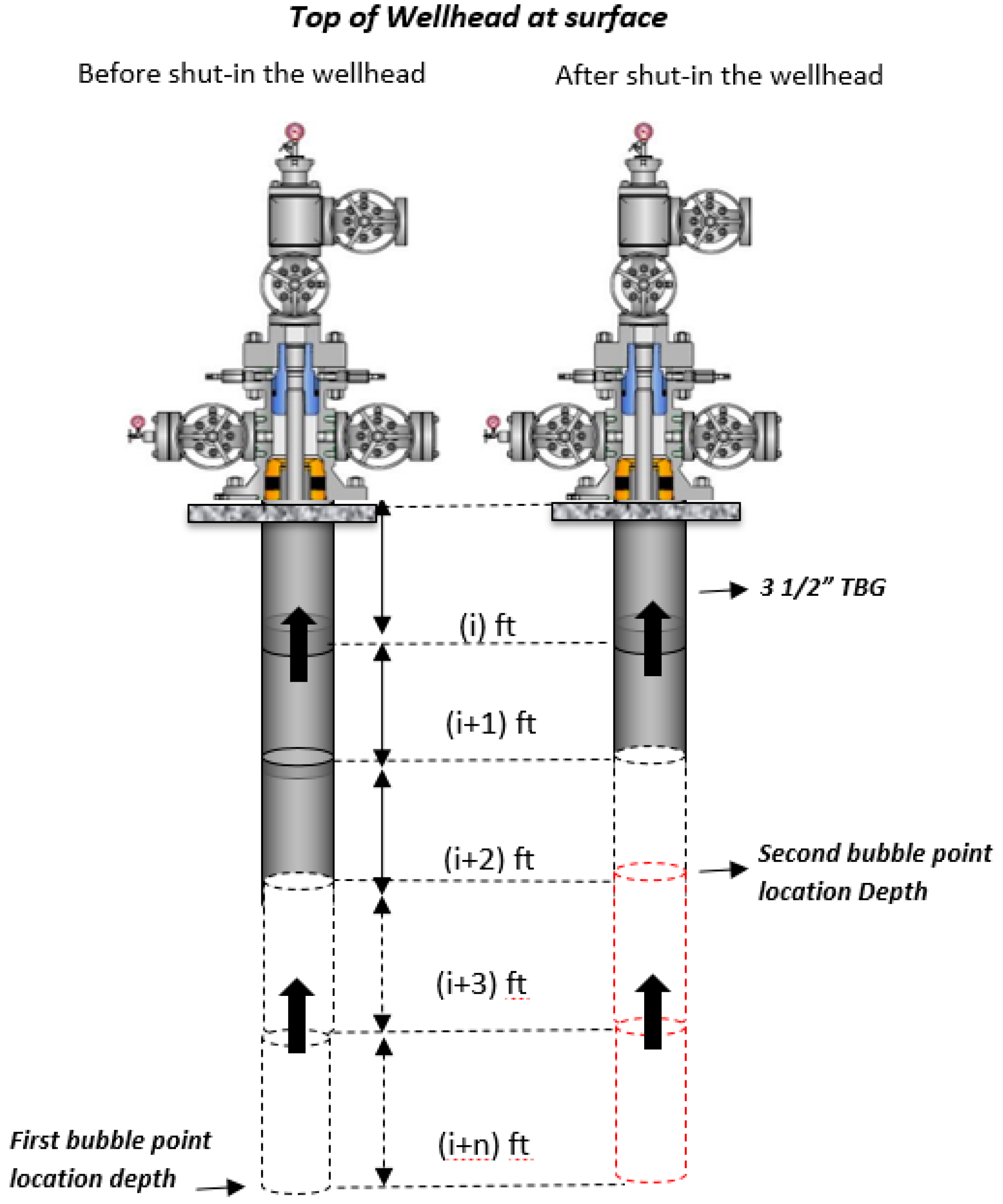
2. Experimental Arrangements and Measurement Procedure
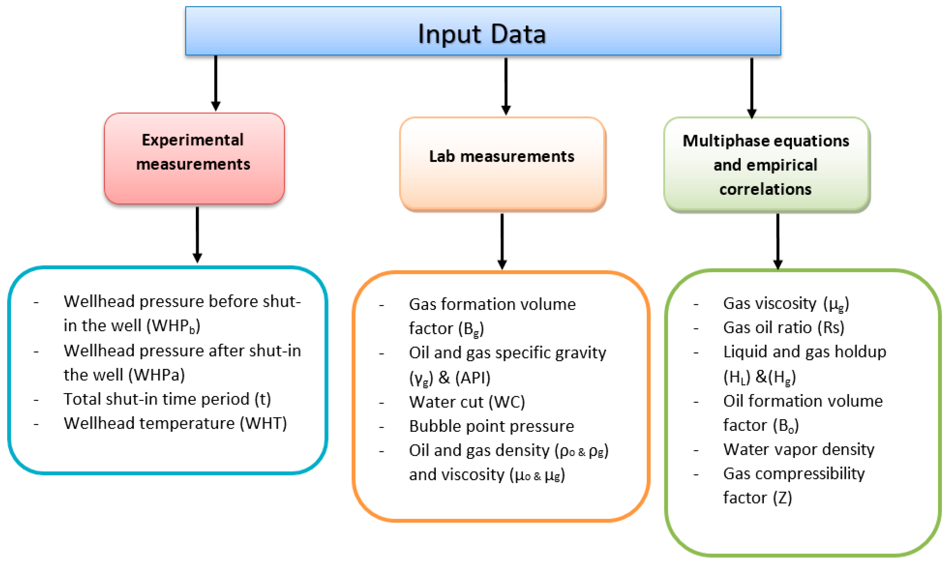
2.1. Required Input Data
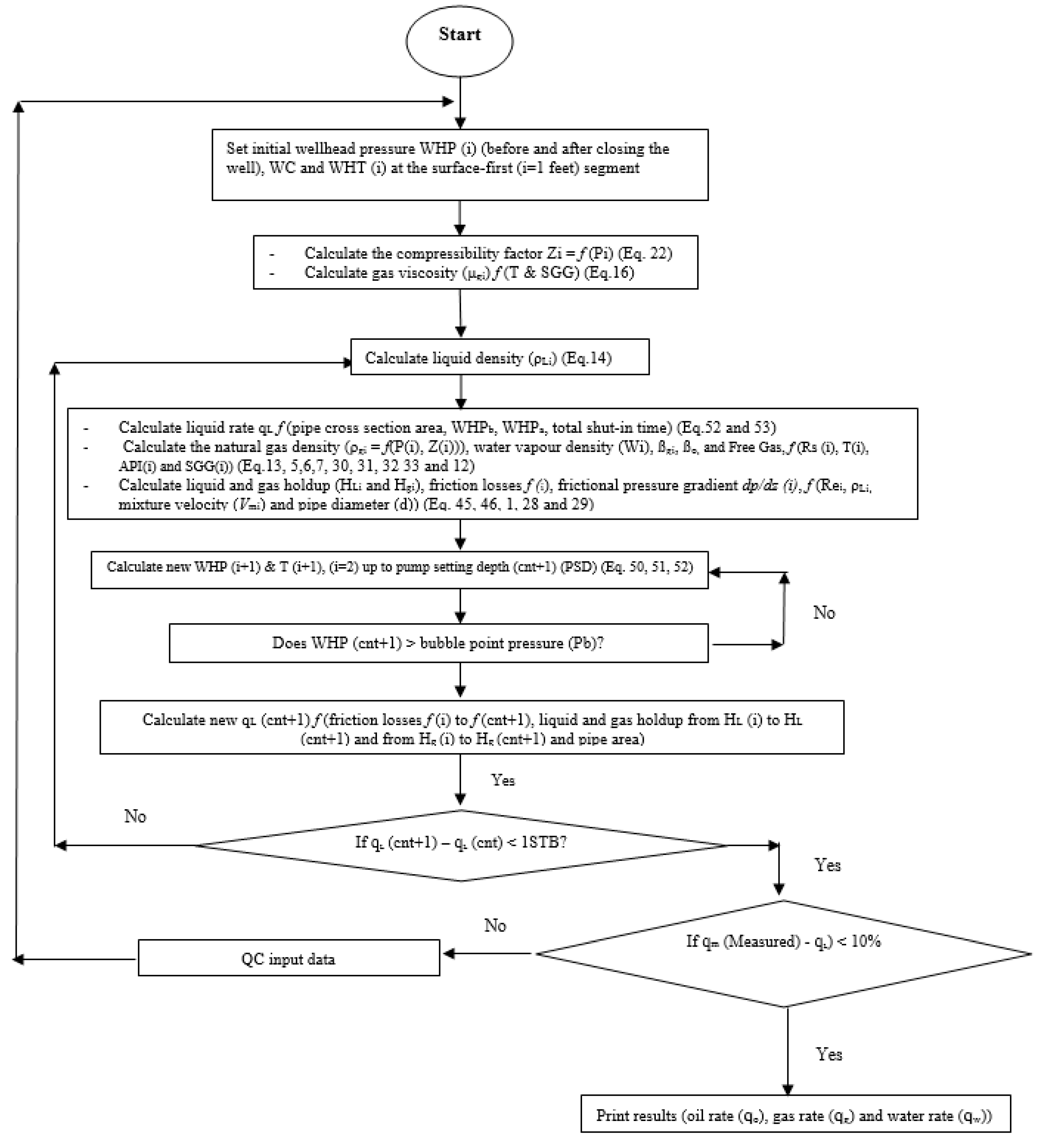
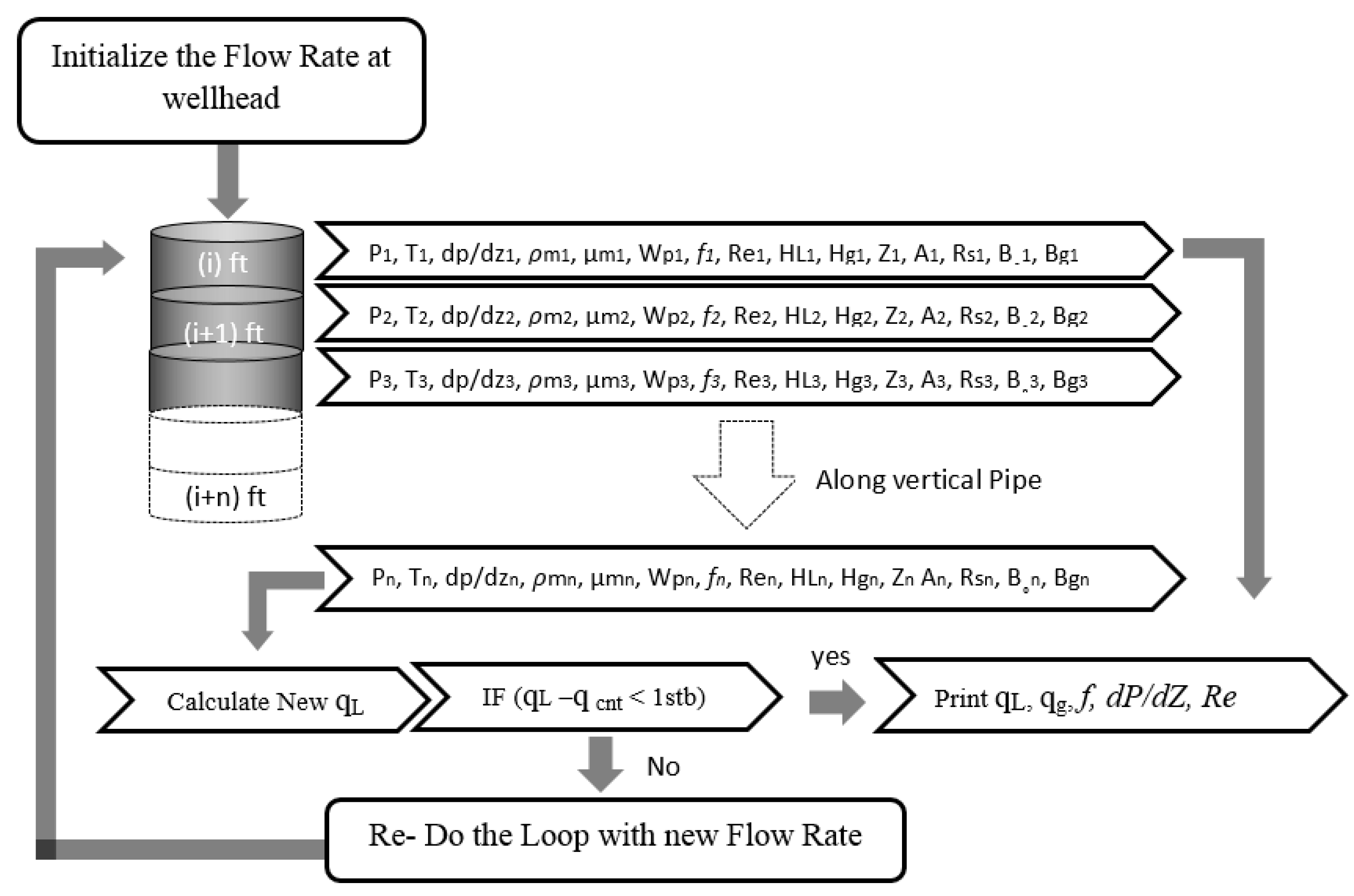
2.2. Computational Algorithm
| Coefficient | °API ≤ 30 | °API ≥ 30 |
| C1 | 27.64 | 56.060 |
| C2 | 1.0937 | 1.187 |
| C3 | 11.172 | 10.393 |
3. Results and Discussion
4. Summary and Conclusions
Author Contributions
Funding
Acknowledgments
Conflicts of Interest
Nomenclature
| A | cross-sectional area, (sq ft) |
| API | American Petroleum Institute |
| Bo | oil formation volume factor, (bbl/stb) |
| Bob | oil formation volume (at bubble point pressure), (bbl/STB) |
| Bg | gas formation volume factor, (cf/scf) |
| Cnt | count |
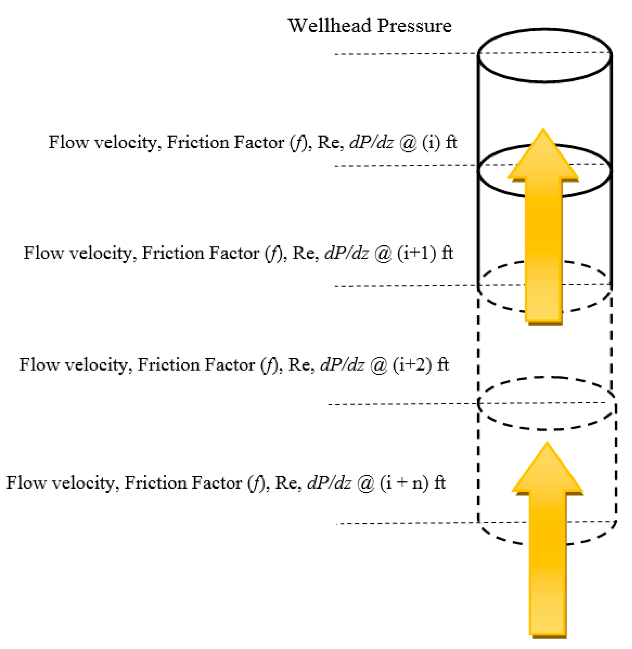
| dp/dz | pressure gradient, (psi/ft) |
| d | inside diameter, (ft) |
| ESP | electrical submersible pump |
| f | friction factor, (unitless) |
| g | Gravity, (ft/s2) |
| HL | liquid hold-up |
| HG | gas hold-up |
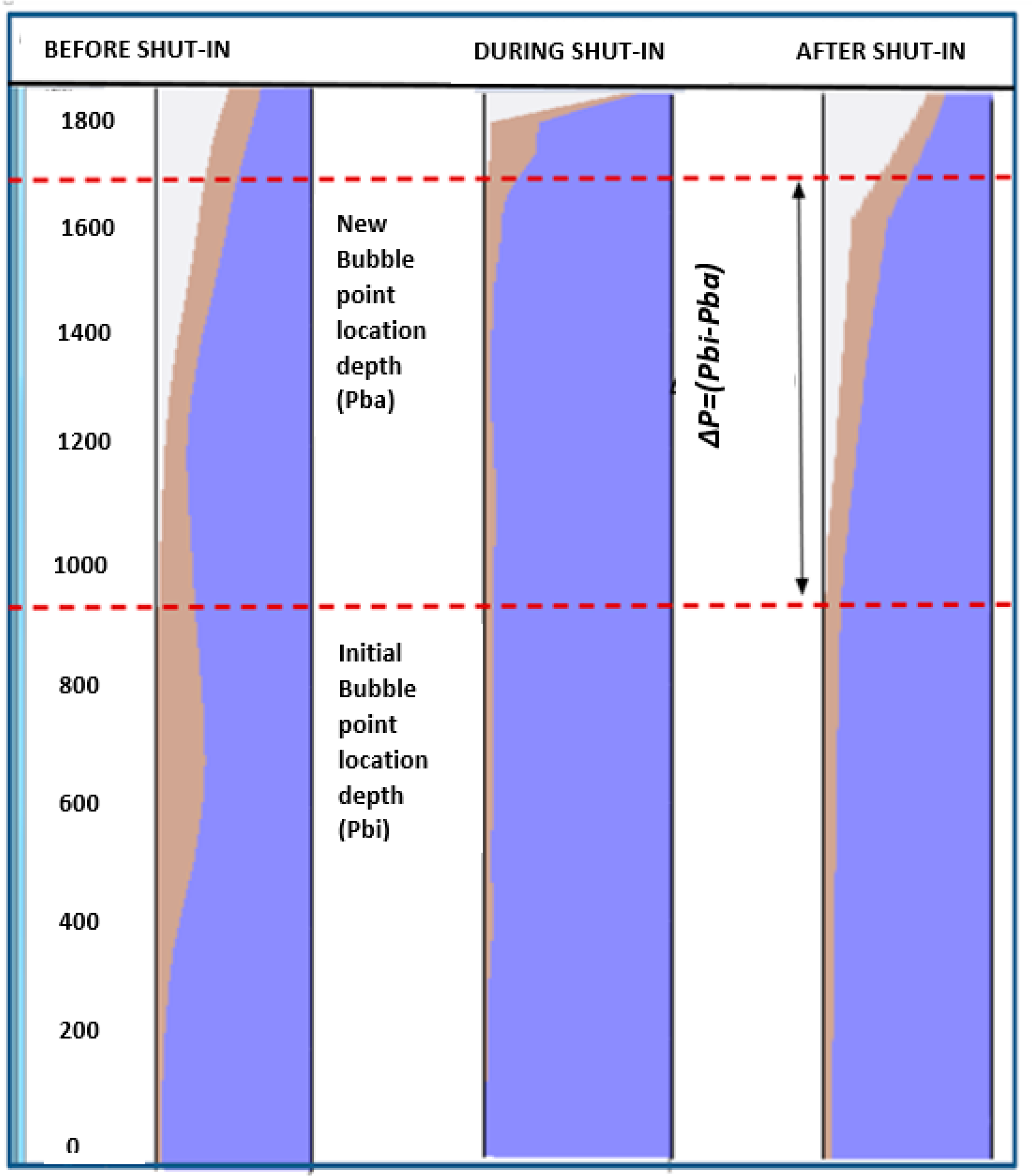
| H1 | bubble point pressure (at location depth before shut-in the well head valve), (ft) |
| H2 | bubble point pressure (at location depth after shut-in the well head valve), (ft) |
| mt | mass flow rate, (lb/day) |
| Ngv | gas velocity number, (unitless) |
| NLv | liquid velocity number, (unitless) |
| Nd | pipe diameter number, (unitless) |
| NCL | coefficient number of viscosity correction, (unitless) |
| NL | liquid viscosity number, (unitless) |
| qo | oil rate, (stb/day) |
| qg | gas rate, (stb/day) |
| qw | water rate, (stb/day) |
| qL | liquid rate, (stb/day) |
| qm | measured flow rate, (stb/day) |
| QC | quality check |
| P | pressure, (psia) |
| Pr | pseudo-critical pressure (for gas mixture), (psia) |
| Pb | bubble point pressure, (psia) |
| Psc | pressure at standard conditions (P = 14.7 atm, T = 60 °F), (psia) |
| PSD | pump setting depth |
| SGG | gas specific gravity |
| STB | stock tank barrel (for liquid) |
| rw | wellbore radius, (ft) |
| Rs | gas-oil ratio, (scf/stb ) |
| Rsb | gas oil ratio at bubble point pressure, (cf/scf) |
| Re | Reynolds number, (unitless) |
| T | temperature, (°F) |
| t | total shut-in time, (min) |
| Tr | pseudo-critical temperature (for gas mixture), (psia) |
| Tsc | temperature at standard condition, (°R) |
| Tr | reservoir fluid temperature, (°F) |
| VR | gas volume at reservoir conditions, (ft3) |
| Vsc | gas volume at standard condition, (ft3) |
| VSL | superficial velocity for liquid, (ft/sec) |
| VSg | superficial velocity for gas, (ft/sec) |
| Vm | total mixture velocity, (ft/sec) |
| WHPa | well head pressure (after shut-in the well), (psia) |
| WHPb | well head pressure (before shut-in the well), (psia) |
| WC | water cut (unitless) |
| WHT | well head temperature, (°F) |
| W | water vapor density, (unitless) |
| Z | gas compressibility factor (unitless) |
| Greek Symbols | |
| ΔP | pressure drop, (psia) |
| HL/ψ | hold-up correlation factor |
| γo | oil gravity |
| γw | water gravity |
| γg | gas gravity |
| σ | surface tension, (dyne/m) |
| ΔH | differences between bubble point pressure location depths (before and after shut-in the well head valve), (ft) |
| ρo | oil density, (lbm/ft3) |
| ρg | gas density, (lbm/ft3) |
| ρw | water density, (lbm/ft3) |
| ρL | liquid density, (lb/ft3) |
| ρm | mixture density, (lbm/ft3) |
| µo | oil viscosity, cP |
| µg | gas viscosity, cP |
| µL | liquid viscosity, cP |
| Subscripts | |
| gsc | gas (at standard condition) |
| h | hydrostatic |
| L | liquid |
| m | mixture (liquid and gas) |
| o | oil |
| sc | standard condition |
| w | water |
References
- Saeb, M.B.; Philip, D.M.; David, C.C.; Ali, J. Modeling friction factor in pipeline flow using a GMDH-type neural network. Cogent Eng. 2015, 2. [Google Scholar] [CrossRef]
- Shannak, B.A. Frictional pressure drop of gas liquid two-phase flow in pipes. Nuclear Eng. Des. 2008, 238, 3277–3284. [Google Scholar] [CrossRef]
- Jiang, J.Z.; Zhang, W.M.; Wang, Z.M. Research progress in pressure-drop theories of gas-liquid two-phase pipe flow. In Proceedings of the China International Oil & Gas Pi (CIPC 2011), Langfang, China, 5 September 2011. [Google Scholar]
- Xu, Y.; Fang, X.D.; Su, X.H.; Zhou, Z.R.; Chen, W.W. Evaluation of frictional pressure drop correlations for two-phase flow in pipes. Nuclear Eng. Des. 2012, 253, 86–97. [Google Scholar] [CrossRef]
- Mittal, G.S.; Zhang, J. Friction factor prediction for Newtonian and non-Newtonian fluids in pipe flows using neural networks. Int. J. Food Eng. 2007, 3, 1–18. [Google Scholar] [CrossRef]
- Fadare, D.A.; Ofidhe, U.I. Artificial neural network model for prediction of friction factor in pipe flow. J. Appl. Sci. 2009, 5, 662–670. [Google Scholar]
- Bilgil, A.; Altun, H. Investigation of flow resistance in smooth open channels using artificial neural networks. Flow Meas. Instrum. 2008, 19, 404–408. [Google Scholar] [CrossRef]
- Özger, M.; Yildirim, G. Determining turbulent flow friction coefficient using adaptive neuro-fuzzy computing techniques. Adv. Eng. Softw. 2009, 40, 281–287. [Google Scholar] [CrossRef]
- Shayya, W.H.; Sablani, S.S.; Campo, A. Explicit calculation of the friction factor for non-Newtonian fluids using artificial neural networks. Dev. Chem. Eng. Miner. Process. 2005, 13, 5–20. [Google Scholar] [CrossRef]
- Yuhong, Z.; Wenxin, H. Application of artificial neural network to predict the friction factor of open channel flow. Commun. Nonlinear Sci. Numer. Simul. 2009, 14, 2373–2378. [Google Scholar] [CrossRef]
- Yazdi, M.; Bardi, A. Estimation of friction factor in pipe flow using artificial neural networks. Can. J. Autom. Control Intell. Syst. 2011, 2, 52–56. [Google Scholar]
- Sablani, S.S.; Shayya, W.H. Neural network based non-iterative calculation of the friction factor for power law fluids. J. Food Eng. 2003, 57, 327–335. [Google Scholar] [CrossRef]
- Griffith, P. Two-Phase Flow in Pipes. In Special Summer Program; Massachusetts Institute of Technology: Cambridge, MA, USA, 1962. [Google Scholar]
- Raxendell, P.B. The Calculation of Pressure Gradients in High-Rate Flowing Wells. J. Pet. Technol. 1961, 13, 1023. [Google Scholar] [CrossRef]
- Fancher, G.H.; Brown, K.E. Prediction of Pressure Gradients for Multiphase Flow in Tubing. Soc. Pet. Eng. J. 1963, 3, 59. [Google Scholar] [CrossRef]
- Hagedorn, A.R.; Brown, K.E. The Effect of Liquid Viscosity in Vertical Two-Phase Flow. J. Pet. Technol. 1964, 16, 203. [Google Scholar] [CrossRef]
- Poettmann, F.H.; Carpenter, P.G. The Multiphase Flow of Gas, Oil and Water through Vertical Flow Strings with Application to the Design of Gas-Lift Installations. In Proceedings of the Drilling and Production Practice, New York, NY, USA, 1 January 1952; Volume 52, p. 257. [Google Scholar]
- Tek, M.R. Multiphase Flow of Water, Oil and Natural Gas Through Vertical Flow Strings. J. Pet. Technol. 1961, 13, 1029. [Google Scholar] [CrossRef]
- Shaban, H.; Tavoularis, S. Identification of flow regime in vertical upward air–water pipe flow using differential pressure signals and elastic maps. Int. J. Multiph. Flow 2014, 61, 62–72. [Google Scholar] [CrossRef]
- Daev, Z.A.; Kairakbaev, A.K. Measurement of the Flow Rate of Liquids and Gases by Means of Variable Pressure Drop Flow Meters with Flow Straighteners. Meas. Tech. 2017, 59, 1170–1174. [Google Scholar] [CrossRef]
- Cai, B.; Guo, D.X.; Jing, F.W. Study on gas-liquid two-phase flow patterns and pressure drop in a helical channel with complex section. In Proceedings of the 23rd International Compressor Engineering Conference, West Lafayette, IN, USA, 11–14 July 2016. [Google Scholar]
- Oliveira, J.L.G.; Passos, J.C.; Verschaeren, R.; Van der Geld, C. Mass flow rate measurements in gas-liquid flows by means of a venturi or orifice plate coupled to a void fraction sensor. Exp. Therm. Fluid Sci. 2009, 33, 253–260. [Google Scholar] [CrossRef]
- Brown, G.O. The history of the Darcy-Weisbach equation for pipe flow resistance. Environment. Available online: https://ascelibrary.org/doi/abs/10.1061/40650 (accessed on 17 September 2018).
- Blasius, H. Das Ähnlichkeitsgesetz bei Reibungsvorgängen in Flüssigkeiten, Mitteilung 131 über Forschungsarbeiten auf dem Gebiete des Ingenieurwesens; Springer: Berlin, Germany, 1913. [Google Scholar]
- Colebrook, C.F. Turbulent flow in pipes, with particular reference to the transition region between the smooth and rough pipe laws. J. Inst. Civ. Eng. 1939, 11, 133–156. [Google Scholar] [CrossRef]
- Lee, A.L.; Gonzalez, M.H.; Eakin, B.E. The Viscosity of Natural Gases. J. Pet. Technol. 1966, 18, 997–1000. [Google Scholar] [CrossRef]
- Beggs, D.H.; Brill, J.P. A study of two-phase flow in inclined pipes. J. Pet. Technol. 1973, 25, 607–617. [Google Scholar] [CrossRef]
- Standing, M.B.; Katz, D.L. Density of natural gases. Trans. AIME 1942, 146, 140–149. [Google Scholar] [CrossRef]
- Sloan, E.; Khoury, F.; Kobayashi, R. Measurement and interpretation of the water content of a methane-propane mixture in the gaseous state in equilibrium with hydrate. Ind. Eng. Chem. Fundam. 1982, 21, 391–395. [Google Scholar]
- Vazquez, M.; Beggs, H.D. Correlations for Fluid Physical Property Prediction. J. Pet. Technol. 1980, 32, 968–970. [Google Scholar] [CrossRef]
- Hagedorn, A.R.; Brown, K.E. Experimental Study of Pressure Gradients Occurring during Continuous Two-Phase Flow in Small Diameter Vertical Conduit. J. Pet. Technol. 1965, 17, 475–484. [Google Scholar] [CrossRef]
- Duns, H., Jr.; Ros, N. Vertical Flow of Gas and Liquid Mixtures in Wells. In Proceedings of the 6th World Petroleum Congress, Frankfurt am Main, Germany, 19–26 June 1963; p. 451. [Google Scholar]
- Orkiszewski, J. Predicting Two-Phase Pressure Drops in Vertical Pipe. J. Pet. Technol. 1967, 19, 829–838. [Google Scholar] [CrossRef]
- Aziz, K.; Govier, G.; Fogarasi, M. Pressure Drop in Wells Producing Oil and Gas. J. Can. Pet. Technol. 1972, 11, 38. [Google Scholar] [CrossRef]


| Well Name | WHPb | WHPa | WHT | GOR | WC | Total Shut-in Time |
|---|---|---|---|---|---|---|
| (PSIA) | (PSIA) | (F) | (SCE/STB) | (%) | (min) | |
| A33 | 140 | 200 | 98 | 360.92 | 93 | 1.55 |
| A125 | 100 | 200 | 95 | 360.92 | 91.62 | 0.83 |
| A64 | 180 | 250 | 107 | 360.92 | 81.52 | 1.06 |
| A29 | 250 | 270 | 107 | 360.92 | 84.88 | 0.80 |
| A23 | 210 | 260 | 127.7 | 360.92 | 82.11 | 0.24 |
| A135 | 210 | 250 | 100 | 360.92 | 59.88 | 0.56 |
| A126 | 250 | 300 | 98 | 360.92 | 66.91 | 0.20 |
| A12 | 175 | 270 | 107 | 360.92 | 82.9 | 0.84 |
| A108 | 260 | 300 | 97 | 360.92 | 81.31 | 0.28 |
| 5J5 | 150 | 300 | 95 | 360.92 | 4 | 3.36 |
| 5J2 | 100 | 170 | 101 | 360.92 | 52 | 1.39 |
| 5J4 | 250 | 300 | 101.6 | 360.92 | 58.95 | 0.27 |
| 5J7 | 250 | 300 | 98 | 360.92 | 30 | 0.47 |
| E89 | 150 | 190 | 140 | 300 | 79 | 0.27 |
| E210 | 80 | 120 | 110 | 300 | 83 | 0.33 |
| E211 | 80 | 120 | 129 | 300 | 74 | 0.96 |
| E286 | 70 | 100 | 146 | 300 | 90 | 0.25 |
| E192 | 80 | 110 | 146 | 300 | 83 | 0.24 |
| E327 | 80 | 110 | 115.5 | 300 | 77 | 0.35 |
| E325 | 70 | 110 | 124.6 | 300 | 83 | 0.44 |
| E197 | 90 | 110 | 146.1 | 300 | 82 | 0.11 |
| E208 | 95 | 110 | 146.8 | 300 | 81 | 0.07 |
| E226 | 80 | 110 | 138.4 | 300 | 91 | 0.25 |
| E284 | 80 | 120 | 124.5 | 300 | 76 | 0.33 |
| E258 | 65 | 90 | 142 | 300 | 86 | 0.23 |
| E326 | 60 | 100 | 113 | 300 | 82 | 0.48 |
| E227 | 100 | 150 | 142 | 300 | 84 | 0.36 |
| 4E_3 | 130 | 300 | 146 | 300 | 87 | 1.18 |
| B56 | 120 | 170 | 120 | 384 | 42 | 2.3 |
| B70 | 160 | 230 | 120 | 384 | 29.9 | 2.9 |
| B121 | 100 | 160 | 120 | 364 | 67.29 | 0.5 |
| B119 | 100 | 160 | 120 | 364 | 76.18 | 1.1 |
| B50 | 180 | 250 | 110 | 364 | 68.65 | 0.55 |
| B88 | 100 | 160 | 110 | 364 | 63.59 | 2.1 |
| B14 | 250 | 270 | 110 | 364 | 76.28 | 0.15 |
| B151 | 180 | 230 | 110 | 364 | 55.78 | 0.66 |
| B164 | 100 | 170 | 120 | 364 | 26.3 | 2.1 |
| B51 | 240 | 310 | 120 | 364 | 59.05 | 0.44 |
| Q89 | 100 | 150 | 120 | 364 | 0 | 3.7 |
| Q21 | 80 | 150 | 120 | 364 | 79.22 | 2.1 |
| Q53 | 80 | 150 | 120 | 364 | 71.41 | 2.3 |
| Q14 | 75 | 130 | 120 | 364 | 74.83 | 1.4 |
| Q100 | 80 | 130 | 110 | 364 | 78.27 | 0.55 |
| Q12 | 80 | 150 | 110 | 364 | 80.33 | 0.58 |
| Q85 | 100 | 150 | 110 | 364 | 18.18 | 2.5 |
| Q82 | 100 | 150 | 110 | 364 | 75.3 | 0.5 |
| Q78 | 80 | 150 | 120 | 364 | 37.27 | 2.5 |
| Q76 | 80 | 150 | 120 | 364 | 80.5 | 1.3 |
| Constants | Value |
|---|---|
| c1 | 28.911 |
| c2 | −9668.146 |
| c3 | −1.663 |
| c4 | −130,823.5 |
| c5 | 205.323 |
| c6 | 0.0385 |
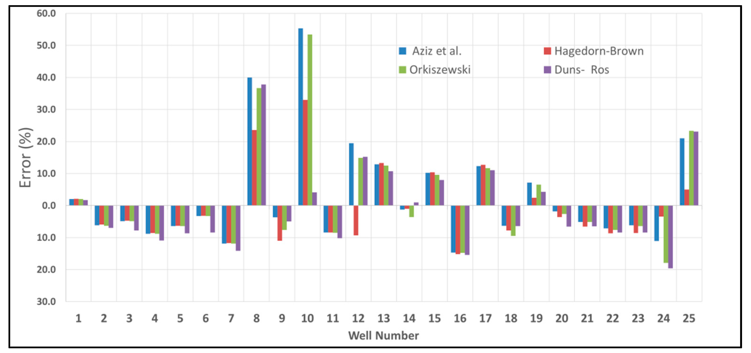
| Prediction Method | Average Error | Standard Deviation |
|---|---|---|
| (%) | (%) | |
| Duns and Ros | −1.06 | 13.06 |
| Hagedorn and Brown | −0.86 | 11.57 |
| Orkiszewski | 1.8 | 16.52 |
| Aziz et al. | 2.9 | 16.66 |
© 2018 by the authors. Licensee MDPI, Basel, Switzerland. This article is an open access article distributed under the terms and conditions of the Creative Commons Attribution (CC BY) license (http://creativecommons.org/licenses/by/4.0/).
Share and Cite
Ganat, T.A.; Hrairi, M. Gas–Liquid Two-Phase Upward Flow through a Vertical Pipe: Influence of Pressure Drop on the Measurement of Fluid Flow Rate. Energies 2018, 11, 2937. https://doi.org/10.3390/en11112937
Ganat TA, Hrairi M. Gas–Liquid Two-Phase Upward Flow through a Vertical Pipe: Influence of Pressure Drop on the Measurement of Fluid Flow Rate. Energies. 2018; 11(11):2937. https://doi.org/10.3390/en11112937
Chicago/Turabian StyleGanat, Tarek A., and Meftah Hrairi. 2018. "Gas–Liquid Two-Phase Upward Flow through a Vertical Pipe: Influence of Pressure Drop on the Measurement of Fluid Flow Rate" Energies 11, no. 11: 2937. https://doi.org/10.3390/en11112937
APA StyleGanat, T. A., & Hrairi, M. (2018). Gas–Liquid Two-Phase Upward Flow through a Vertical Pipe: Influence of Pressure Drop on the Measurement of Fluid Flow Rate. Energies, 11(11), 2937. https://doi.org/10.3390/en11112937