One-Hour Prediction of the Global Solar Irradiance from All-Sky Images Using Artificial Neural Networks

Abstract

We present a method to predict the global horizontal irradiance (GHI) one hour ahead in one-minute resolution using Artificial Neural Networks (ANNs). A feed-forward neural network with Levenberg–Marquardt Backpropagation (LM-BP) was used and was trained with four years of data from all-sky images and measured global irradiance as input. The pictures were recorded by a hemispheric sky imager at the Institute of Meteorology and Climatology (IMuK) of the Leibniz Universität Hannover, Hannover, Germany (52.23° N, 09.42° E, and 50 m above sea level). The time series of the global horizontal irradiance was measured using a thermopile pyranometer at the same site. The new method was validated with a test dataset from the same source. The irradiance is predicted for the first 10–30 min very well; after this time, the length of which is dependent on the weather conditions, the agreement between predicted and observed irradiance is reasonable. Considering the limited range that the camera and the ANN can “see”, this is not surprising. When comparing the results to the persistence model, we observed that the forecast accuracy of the new model reduced both the Root Mean Square Error (RMSE) and the Mean Absolute Error (MAE) of the one-hour prediction by approximately 40% compared to the reference persistence model under various weather conditions, which demonstrates the high capability of the algorithm, especially within the first minutes.

1. Introduction

The production of solar energy is subject to strong spatial and temporal fluctuations due to the dependence on meteorological boundary conditions. This leads to uncertainties in the planning of energy supplies and, thus, to economic inefficiencies. With a reliable solar performance forecast, uncertainty is minimized while load and storage management can be optimized. Thus, prediction of solar irradiation makes an important contribution to efficient and economical applications for many areas of solar energy use, while high-quality one-minute data series are key to understanding the dynamic interaction of photovoltaic (PV) systems, loads, and grids [1].

Worldwide, the installed PV power increases by a double-digit percentage per year [2]. This trend makes photovoltaics an even more important alternative for global power supply. New models for the forecast of solar energy production can help to reduce the difficulties of integrating PV systems into existing power supply structures. In order to optimally manage the power supply, electricity producers are compelled to provide a forecast of the expected delivery quantities [3]. With the help of reliable predictive models, the market price of the solar energy is then determined by supply and demand.

Many solar applications such as PV systems and grid regulation depend critically on the ability to predict cloud movement [4,5]; therefore, sky cover information is a potentially useful input for improving the prediction accuracy of the energy feed-in of solar power systems [6].

Other techniques for predicting solar irradiation are methodologies employing the temporal evolution of all-sky images. Most prediction methodologies focus on cloud identification and motion. Alonso-Montesinos et al. [7] and Marquez and Coimbra [8] achieved this by detecting cloud motion vectors from all-sky images for forecasting short-term predictions of solar radiation. Sky coverage information provided by all-sky images has been successfully used for forecasting minutes ahead of solar irradiance. The results of this investigation showed an accuracy above 17% over the persistence model [9]. In addition, a study by Chow et al. [10] showed that the maximum possible forecast horizon with all-sky images was highly dependent on cloud speed.

Wu and Chan [11] compared a linear statistical autoregressive–moving-average (ARMA) model, a nonlinear artificial neural network (ANN) model, and a hybrid model between both, and they found that the deviation of the data in the ARMA was higher than that in the ANN. ARMA provided a better result for linear components, while the ANN showed a smaller deviation for nonlinear components. ARMA showed better predictions at very low irradiance, while the neural network performed better at high irradiance. The study by Kamadinata et al. [12] developed and compared two different simple methodologies utilizing two ANNs. The first one predicted cloud movement direction, while the second ANN predicted solar radiation using the output of the first ANN as input.

The persistence model is the most common reference model for short-term forecasting of solar irradiance [13,14]. This model supposes that the data at x_t+1 equals the data at x_t. Generally, for solar irradiation predictions, the persistence model is unreliable for forecasting more than one hour in advance [15,16].

The study we present here shows that by applying our method, the solar irradiance can be estimated in one-minute resolution by simulating one hour ahead at the Institute of Meteorology and Climatology (IMuK), Leibniz Universität Hannover, Hannover, Germany. In addition, this study does not require meteorological inputs such as, e.g., humidity, wind speed, or air temperature. Therefore, in further studies the new algorithm could be applied under diverse weather conditions elsewhere.

2. Methods

We developed a new algorithm to predict future data based on observed data, i.e., time series of 60 one-minute values of the global horizontal irradiance and, as their sum, the total amount of energy one hour ahead. It was based on a four-year dataset of all-sky images and the respective thermopile pyranometer measurements that were used as input to machine learning methods.

The algorithm consisted of three main steps. The first part comprised the data preparation for an image processing program and the creation of a program to export pyranometer measurements for the input parameters (Section 2.1). Figure 1 shows the forecast process of the global horizontal irradiance (GHI) with all-sky images and an ANN.

The second part of the study was the creation of three different ANN programs. The Cloud Locating and Cloud Movement Program (Section 2.2), the AllPicture Program, and the RingPicture Program (Section 2.3). The third part consisted of the validation of the new model (Section 2.4).

Table 1. Summary of data preparation and methodology. Step I-selected inputs and the Cloud Movement program. Step II-two different ANNs with their respective inputs and output parameters. Step III-comparison of the neural network and the persistence model. The sun zenith angle (SZA) is the angle between the zenith and the centre of the sun’s disc.

Step	Task	Input	Output
Step 1 (a)	Extraction of parameters from all-sky images as input for next steps.	RGB channel statistics ○ Average ○ Mode ○ Median ○ Standard deviation Sky cover (%) Clouds in the sky (%)
	Extraction of two extra inputs for next steps	GHIMea SZA
Step 1 (b)	Cloud Locating and Cloud Movement program (works with an ANN)	All-sky images Current position of the clouds	Cloud position one minute ahead
Step 2 (a)	Creation of the AllPicture program (preconditioning for seasonal and diurnal variations)	For each image: RGB channel statistics ○ Average ○ Mode ○ Median ○ Standard deviation Sky cover (%) Clouds in the sky (%) GHIMea SZA Cloud position one minute ahead	GHISim
Step 2 (b)	Creation of the RingPicture program	For each ring: RGB channel statistics ○ Average ○ Mode ○ Median ○ Standard deviation Sky cover (%) Clouds in the sky (%) GHISim SZA Cloud position one minute ahead	GHISimFinal
Step 3	Validation	ANN model output Persistence model output	60 one-minute values Hourly sum Deviations

shows the preparation and methodology of these three steps.

2.1. Setup of the ANN

Different numbers of neurons for the input parameters for the three ANN programs were used; see

Table 2. The neural network structure used to carry out this investigation.

ANN Programs	No. of Input Parameters	No. of Hidden Layers	No. of Neurons in the First Hidden Layer	No. of Neurons in the Second Hidden Layer	No. of Output Neurons
Cloud Locating and Cloud Movement program	8	2	4	2	1
AllPicture program	9	2	7	5	1
RingPicture program	9	2	7	5	1

. The Cloud Locating and Cloud Movement program used eight inputs and one output, while the AllPicture and the RingPicture programs each used nine inputs and one output.

Finally, two hidden layers with varying numbers of neurons were necessary for each network. The number of hidden neurons in a single hidden layer was calculated by Equation (1):

$$m=\sqrt{n+l}+\alpha ,$$

(1)

where $n$ is the number of input parameters and $l$ is the number of output neurons; $\alpha$ is a constant ranging between 1 and 10.

In an ANN, the connection between input, hidden, and output neurons was established by synaptic weights and transfer Equation (2). The input information $x_j$ flows through connections that multiply its strength by a weight $w_{i,j}$ to reach a product $w_{i,j}{x}_j$. This product is the argument for a transfer function $f$ that gives the output $y_i$.

$$y_i=f({\displaystyle \sum _{j=1}^n}{w}_{i,j}{x}_j)$$

(2)

The activation function $f$ defines the output of a neuron in terms of the induction of the linear field $y_i$. The activation function calculates the state of activation of a neuron, transforming the global input into a state of activation.

The Levenberg–Marquardt (LM) algorithm, a combination of the Grade and the Gauss–Newton method, was used as learning algorithm. It was used as it is less time consuming and also has the local convergence of the Gauss–Newton method and the complete properties of the Grade method [17].

2.2. Image Acquisitition and Data

The results of Toshing et al., 2013 [18] demonstrated the development of a camera system at IMuK, where the projection of the camera system was found to be nearly equidistant. The pictures for this study were recorded with both a Canon G10 and a Canon EOS 700D, using an exposure time of 1000/s. The Hemispherical Sky Imager (HSI), installed on the roof of IMuK, comprises commercial compact CCD (charge-coupled device) cameras equipped with a fish-eye lens providing a 183° field of view. The maximum image size is 4416 × 3312 pixels, corresponding to 3.5 million pixels for the hemispherical image with a radius of 1060 pixels. In addition, the global irradiance was measured simultaneously using a CMP11 pyranometer (Kipp & Zonen, Delft, The Netherlands), [19].

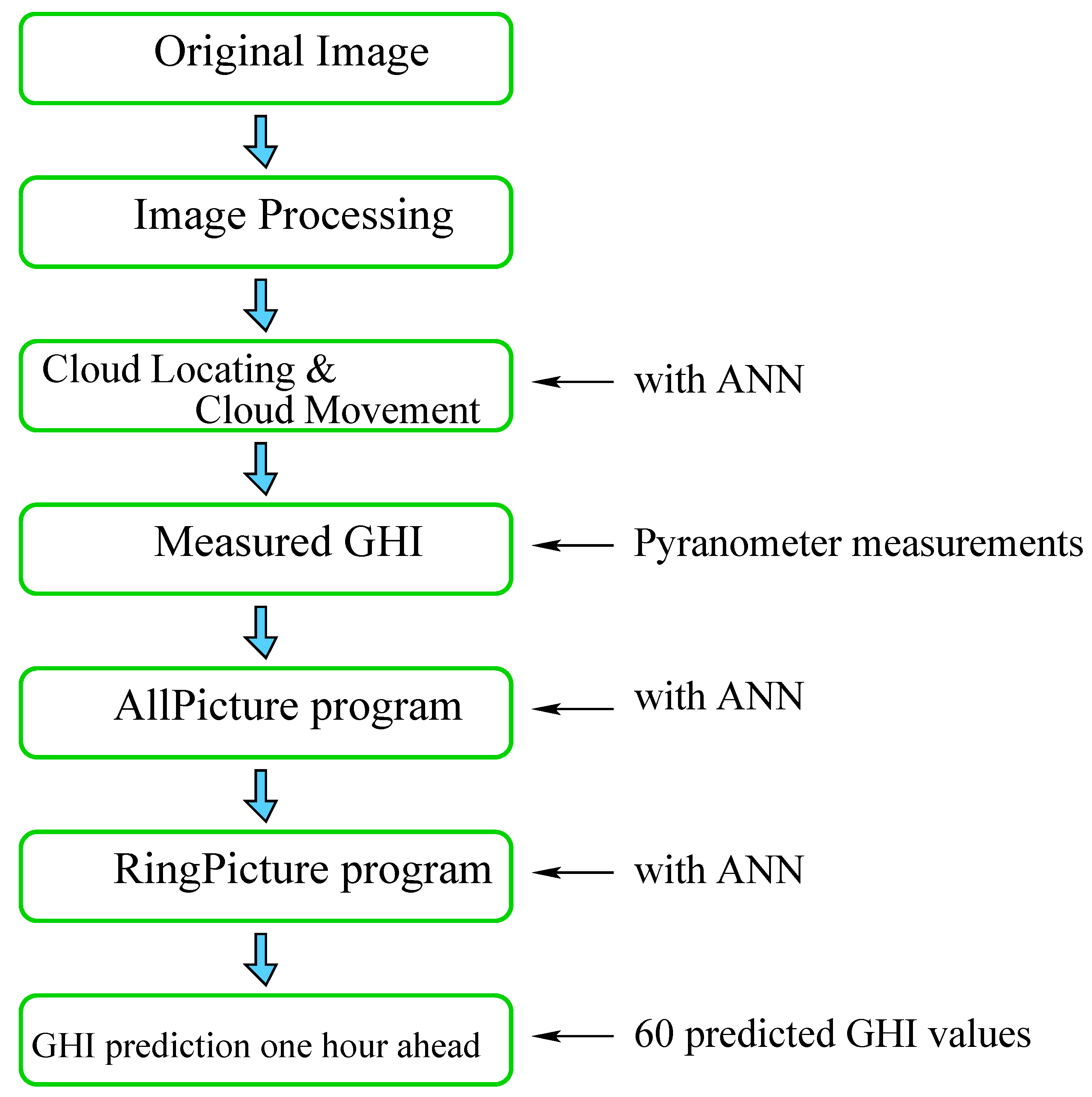
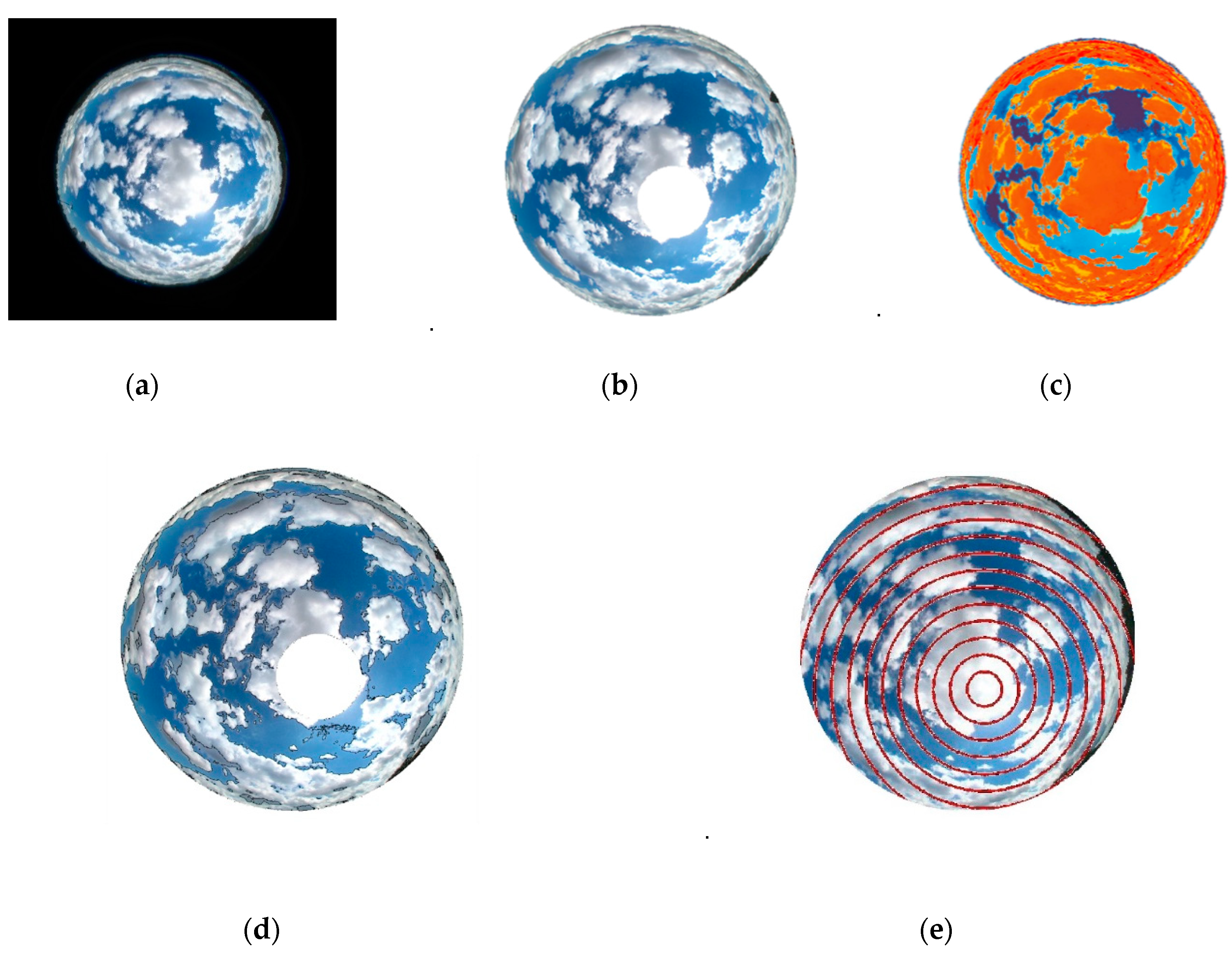
2.3. Images Preprocessing

A software program capable of identifying the area of the sky covered by clouds was developed and used at IMuK. The work of Yamashita et al. [20] permitted the calculations of the sky index from an original picture. However, in this study we calculated the Haze Index (Equation (3)), as stated by Schrempf [21], to improve the cloud identification on the basis of the sky index. An example of the haze index is displayed in Figure 2c.

$$HazeIndex=\frac{\frac{coun{t}_{red}+coun{t}_{blue}}{2}-coun{t}_{green}}{\frac{coun{t}_{red}+coun{t}_{blue}}{2}+coun{t}_{green}}$$

(3)

The Sun Zenith Angle (SZA) algorithm (a free Matlab (Matlab_R2016b) code sample [22]) was extended at IMuK for this study. The output of this program was one-minute solar position values for the location at IMuK. The SZA was the most important input parameter for training the network and for delivering the output parameters in the simulation phase.

2.4. Cloud Locating and Cloud Movement Program

To obtain two new input parameters for the next steps, it was necessary to create an algorithm capable of detecting clouds and predicting their movements. A cloud detection algorithm was used to determine the percentage of clouds in the sky. This method provided automated cloud detection operating in the red and blue channels [23] using super-pixel segmentation [24].

The total sky and cloud area were calculated followed by the percentage of clouds present, i.e., with help of the Haze Index. The cloud pixels were then identified as they were needed to find the cloud locations. If cloud pixels were high, the algorithm drew a contour around the cloud area until the density decreased in the side areas. At low cloud pixels, the algorithm recognized this as a boundary of the cloud.

In our system, as the output parameter, the ANN learned to predict the position of the clouds one minute ahead by combining the movement between Figure 2d,e. The idea was to predict when the clouds would appear in front of the sun, as shown in Figure 2d. The algorithm follows the clouds from the horizon to the center of the sun, taking information from each ring.

Accordingly, the input parameters for the Cloud Locating and Cloud Movement program were the SZA; measured global horizontal irradiance (GHI_Mea); current cloud position (derived from the actual image as described before); percentage of clear sky; percentage of clouds in the sky; and the mathematical average, mode, median, and standard deviation of the RGB channels. The output parameter was the cloud position for the next minute. This output parameter was introduced as an input parameter for the next ANN. The statistical information of each channel and the percentage of clear sky and cloud cover were obtained without taking into consideration the sun’s circumference to avoid oversaturation of the pixels (Figure 2b). In addition, the extraction of the statistical information from the pictures was limited to the time from sunrise to sunset.

2.5. Creation and Training of the AllPicture Program and RingPicture Program

In this step, we created two new ANNs with respective training and simulation processes. A comparison between the different models in terms of training time and prediction deviation indicated that the LM algorithm was the most efficient prediction model. The selection of this learning algorithm was especially important for the training and simulation time processes. The input datasets were divided into 36 months for the training phase and 6 months for the validation.

The simulation of the AllPicture program was preconditioned with training runs on whole images. The input parameters of this ANN were SZA; GHI_Mea; percentage of clear sky; percentage of cloud cover; average, mode, median, and standard deviation of the RGB channels; and cloud position for the next minute. The output of this ANN was the GHI_Sim, and it was used as input to the next ANN, the RingPicture program. Since no time-based information was used in this algorithm, the aim of this ANN preconditioning was to allow it to learn the seasonal and diurnal variations of the solar irradiance.

The second step was the simulation of the RingPicture program, where the actual simulation of the 60 one-minute values takes place. The input parameters of this ANN were SZA; GHI_Sim; percentage of clear sky; percentage of cloud cover; average, mode, median, and standard deviation of the RGB channels; and cloud position for the next minute. The training target and, hence, the most important output of the algorithm was the hourly GHI_SimFinal, calculated as the sum of the 60 one-minute values. Thus, while the AllPicture program worked over the whole picture, the RingPicture program worked over each ring of the picture, i.e., the program considered each ring as a picture (see Figure 2e).

For the simulation of the 60 one-minute values and the resulting hourly GHI_SimFinal, only one image was needed. The image was subdivided into concentric rings around the sun (Figure 2e). The rings had a temporal resolution of one minute; the width depended on the distance from the horizon due to the equidistant projection. For each ring, the same statistical information from the first step was extracted, while the SZA was also adjusted according to the progress in time that the ring represents. With these inputs and the GHI_Sim of the whole image from the first step of Part 2, the ANN simulated the GHI of each ring. Ring after ring was simulated subsequently, starting from the center of the sun and moving to the horizon. The number of simulated minutes, $\mathrm{n}$, depended on the cloud position and the position of the sun.

After the last ring was processed, the calculation method changed in order to calculate the missing one-minute values from $n$ to 60. The statistical information of the last ring was taken and searched for in the database of recorded images. The image that best matched the statistical information was selected, taking into consideration the sun position, time of year, and time of day. To simulate GHI_SimFinal at n + 1, the image was processed. This process was repeated until all 60 values had been generated.

The total GHI_SimFinal for one hour was calculated as the sum of the 60 one-minute values and compared to the measured GHI_Mea value. The deviation was fed back to the ANN until the deviation reached a defined minimum threshold.

2.6. Validation of the New Model

The persistence model assumes that the global irradiation data at x_t is similar to the global irradiation data at x_t-24h, This model was very useful for benchmarking other methods [25]. We assumed that an average of seven days was sufficient to predict the irradiance with the persistence model. When considering only one day, the persistence model would be influenced too much by the current variability. When considering more than seven days, the simulation did not improve any further.

Figure 3 shows the persistence model’s forecast for two days in more detail. This model processed the information to the end time of the desired simulation. On the day of the simulation, the persistence model processed the information just until the simulation began, thus delivering the simulated hour.

3. Results

The following days were selected for validating the new algorithm: 18 September 2014; and 10 January, 14 August and 21 August, 2015. The selected days represented different weather conditions with high solar irradiance variability. The root-mean-square error (RMSE) (Equation (4)), mean absolute error (MAE) (Equation (5)), and the coefficient of determination (R²) (Equation (6)) were used to evaluate the performance of the new model for these four days. In addition, 17 July 2015 was selected to simulate 13 h from 05:01 to 18:00. Definitions are expressed as follows:

$$\mathrm{RMSE}=\sqrt{{\sum }_{i=1}^N\frac{\Vert y_i-x_i\Vert }{N}},$$

(4)

$$\mathrm{MAE}=\frac{{\sum }_{i=1}^N\left|y_i-x_i\right|}{N},$$

(5)

$${\mathrm{R}}^2={\sum }_{i=1}^N\left(y_i-\overline{y}\right)\left(x_i-\overline{x}\right)/{[({\sum }_{i=1}^N{\left(y_i-\overline{y}\right)}^2)({\sum }_{i=1}^N{\left(x_i-\overline{x}\right)}^2)]}^{1/2},$$

(6)

where y_i is the forecast value, x_i is the measured value, and N is the number of samples. Additionally, $\overline{x}={\sum }_{i=1}^N{x}_i$ and $\overline{y}={\displaystyle \sum _{i=1}^N}{y}_i$. Finally, to validate our model, i.e., for knowing how many simulations we had to carry out for the validation of the new model, statistical sampling (Equation (7)) was utilized, and the results are presented as a boxplot. The definition of the statistical sampling is expressed as follows:

$$x=\left(Z^{2}Npq\right)/\left(e^2\left(N-1\right)Z^{2}pq\right),$$

(7)

where N is the total of the set, p = 0.95, q = 0.05, and Z = 1.96 (this value corresponds to the confidence level of 95%).

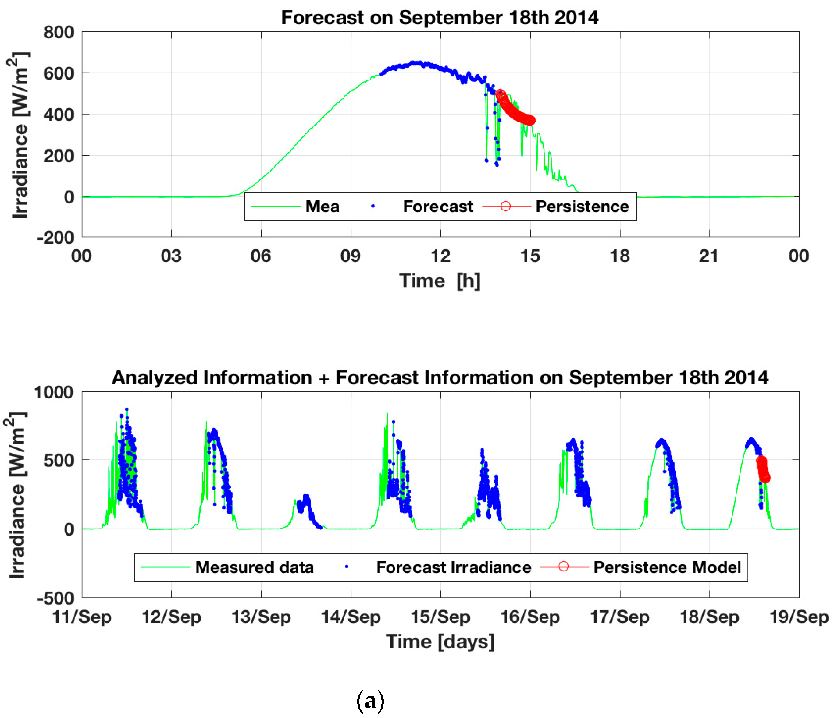
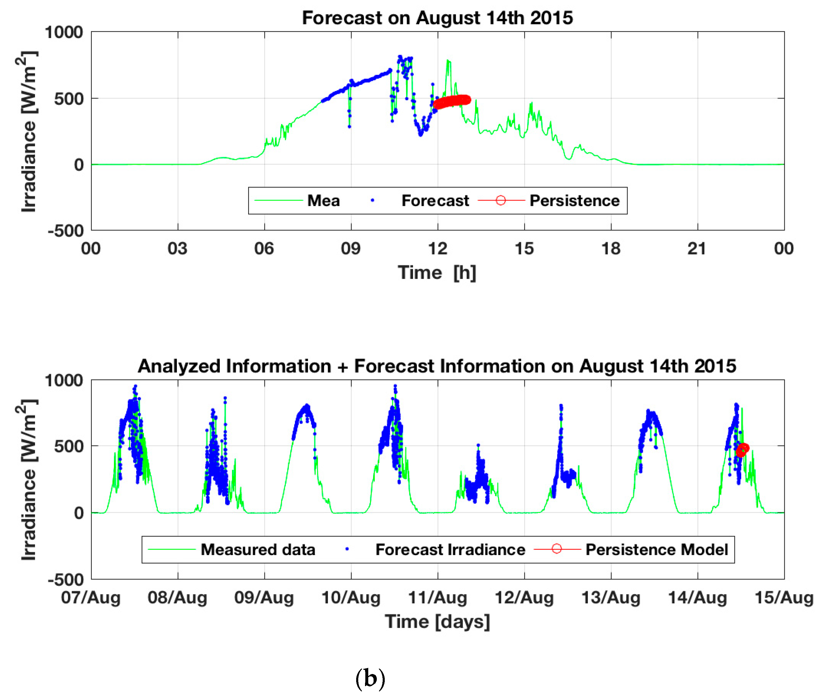
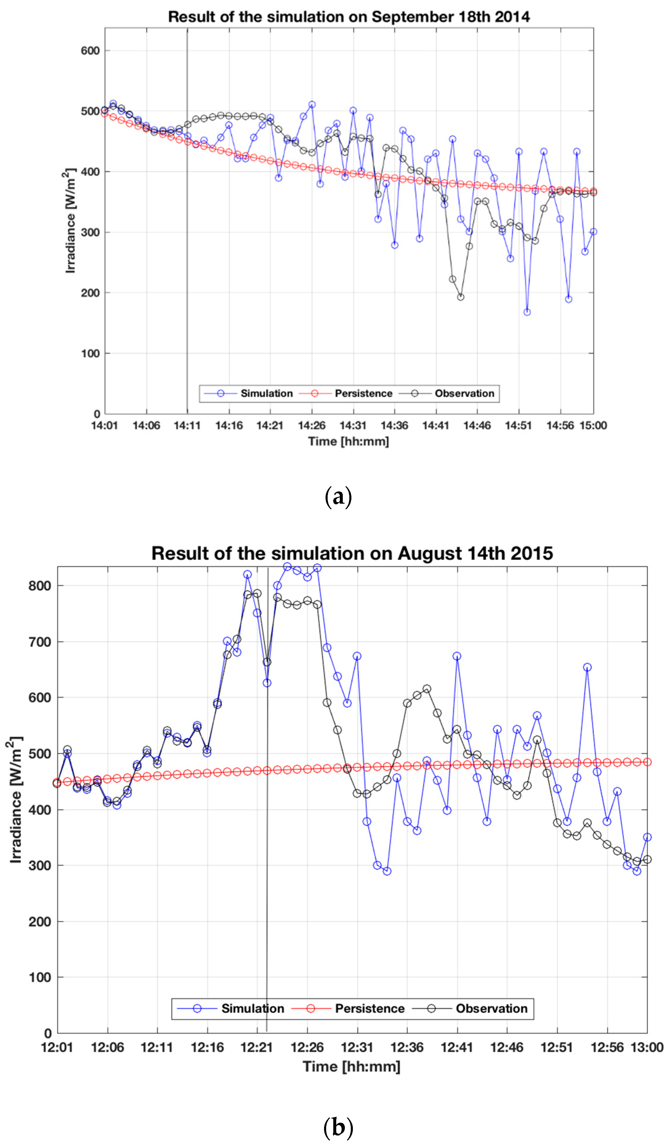
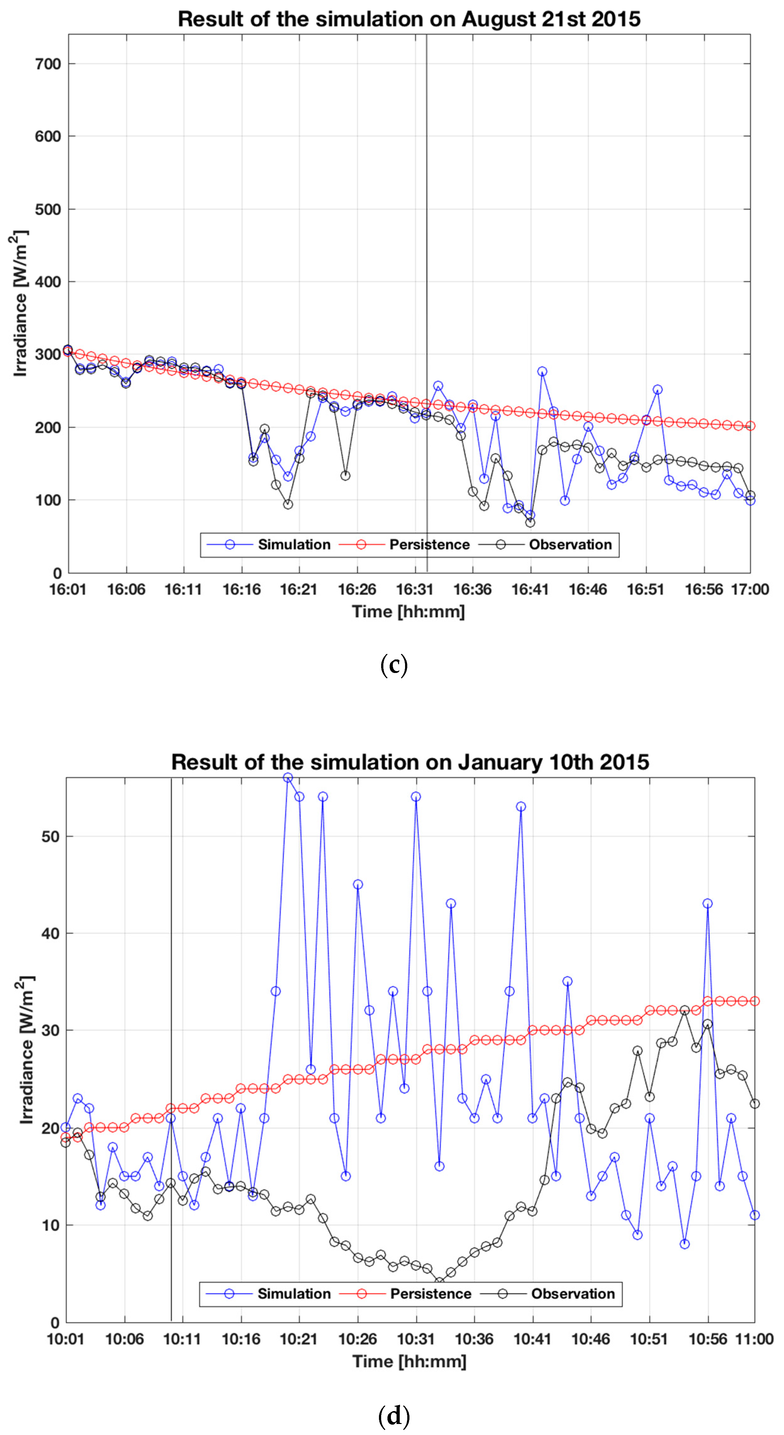
3.1. Analysis of One-Hour-Ahead Results

Figure 4 shows the forecasts of one-hour-ahead simulation for four days using the new algorithm and the persistence model. These values were compared with the measured data. The results show that the forecast values of the ANN model closely matched the measured values, and both the RMSE and the MAE were smaller in the new ANN model than in the persistence model for the entire simulated hour (see

Table 3. Comparison of the statistical indicators of the new ANN forecast model against the persistence forecast model on four different days. The table compares the information until the last picture with the information after the last picture.

Simulation day	Models to compare	With Information from the Last Picture				When the Last Picture Does Not Provide Information Anymore
Day	Model	Minutes	RMSE (Wh/m2)	R2	MAE (Wh/m2)	Minutes	RMSE (Wh/m2)	R2	MAE (Wh/m2)
18 Sepetember 2014	ANN	11	7	0.92	5	49	77	0.52	61
	Persist		14	0.85	12		69	0.38	98
14 August 2015	ANN	22	12	0.99	8	38	111	0.77	90
	Persist		111	0.77	74		149	0.13	116
21 August 2015	ANN	32	21	0.92	10	28	49	0.55	39
	Persist		51	0.58	29		72	0.17	65
10 Jane 2015	ANN	10	4	0.78	3	50	20	0.42	16
	Persist		7	0.71	6		14	0.64	13

and

Table 4. Summary of the statistical indicators of the new ANN forecast model for four different days.

Day	Hour	Total Measured Energy (Wh/m2)	Total Simulated Energy (Wh/m2)	Difference (Wh/m2)	RMSE (Wh/m2)	R2	MAE (Wh/m2)
18 September 2014	14:01–15:00	414.8	412.3	2.5	69	0.61	50
14 August 2015	12:01–13:00	510	521	11	91	0.79	62
21 August 2015	16:01–17:00	197	203	6	37	0.84	24
10 January 2015	10:01–11:00	15	24	9	19	0.38	14

).

The new algorithm was able to produce forecasts of higher quality compared to the reference persistence model, even when it stopped receiving information from the last picture. The last pictures were taken at 14:00 on 18 September 2014, at 12:00 on 14 August 2015, at 16:00 on 21 August 2015 and at 10:00 on 10 January 2015 and provided the algorithm with 11, 22, 32, and 10 min of future information, respectively. The most important improvement was the decrease in RMSE and MAE of the total energy received at the surface over one hour. Figure 4d shows a particular simulation case where the measured irradiance was very low—between 4 W/m² and 32 W/m². Under low irradiance conditions, the network did not predict adequately when it stopped receiving information from the last taken picture; see Table 3. The measured irradiation value at IMuK on 10 January, 2015 was 15 Wh/m² between 10:01 and 11:00. Our model simulated a total of 24 Wh/m², i.e., a difference of 9 Wh/m² (54%). In comparison, the persistence model predicted a total of 27 Wh/m², a difference of 12 Wh/m², which corresponds to 76%. The new model does not significantly outperform the persistence model. For very small irradiance levels, the ANN does not have the same effectiveness as for high irradiance levels. However, forecasts with very low irradiance levels were of minor relevance for solar energy forecasts. On September 18, 2014, from 16:01 to 17:00, the irradiation measured at IMuK was 414.8 Wh/m² and the new model simulated 412.3 Wh/m², which corresponds to a difference of 2.5 Wh/m² (0.06%). The persistence model predicted 408.3 Wh/m² with a difference of 6.5 Wh/m², corresponding to 1.6% (Table 3 and Table 4).

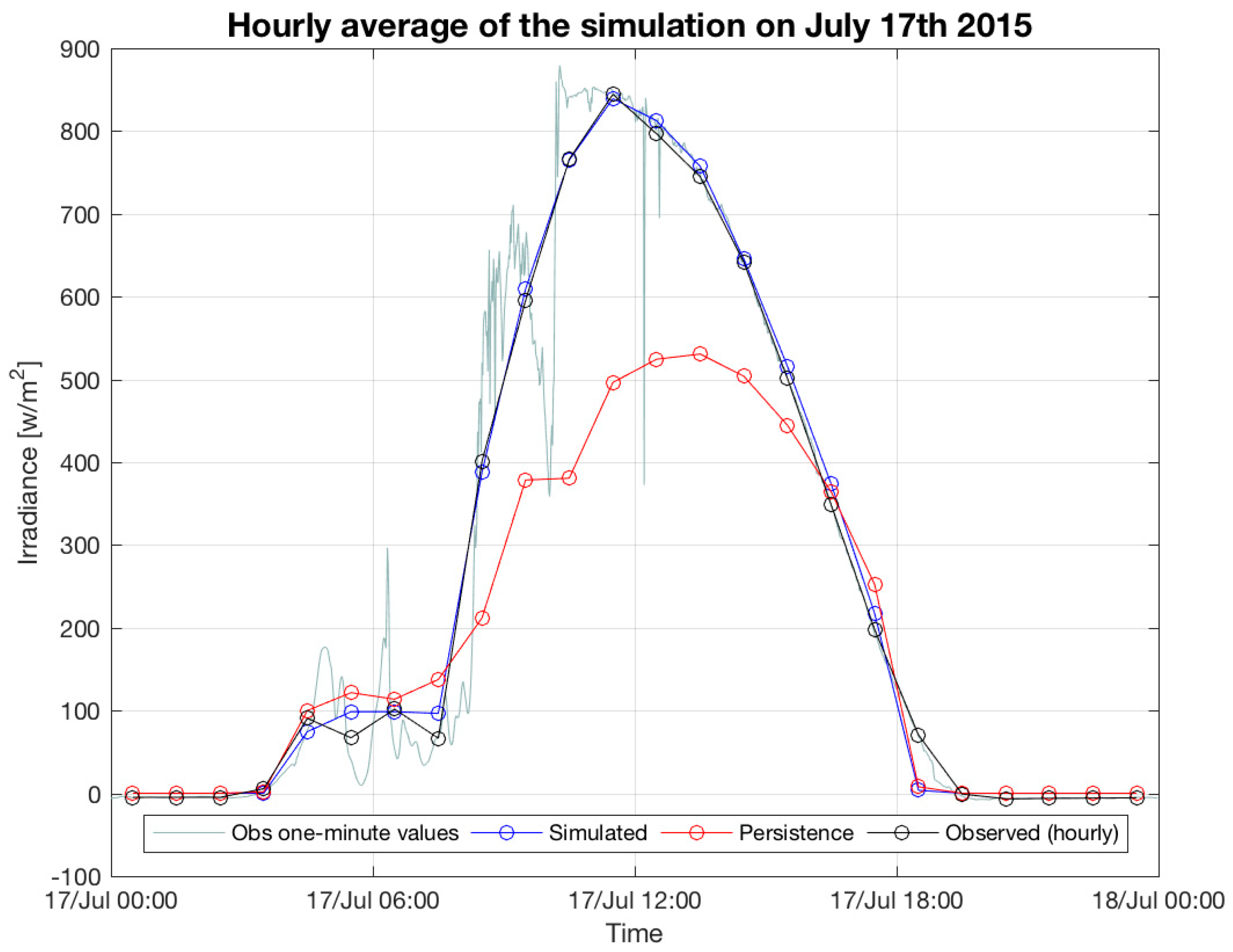
3.2. Analysis of the Daily Integrated Irradiation

The hourly average of the simulation for one day on 17 July 2015 from 05:01 to 18:00 is shown in Figure 5. When making a prediction for an entire day, it was necessary to take a picture every 60 min.

In Figure 5 we see that the persistence model, as a linear statistical model, cannot describe the performance for days with broken clouds as accurately as the new ANN model can.

Table 5. Comparison of the statistical indicators of the ANN forecast model against the persistence forecast model on 17 July 2015 at 05:01 to 18:00.

Model	RMSE (Wh/m2)	R2	MAE (Wh/m2)
ANN	65	0.98	30
Persistence	91	0.91	63

compares the statistical indicators of the global irradiance for the one-hour prediction on 17 July 2015 from 05:01 to 18:00 using the new ANN model and the persistence model.

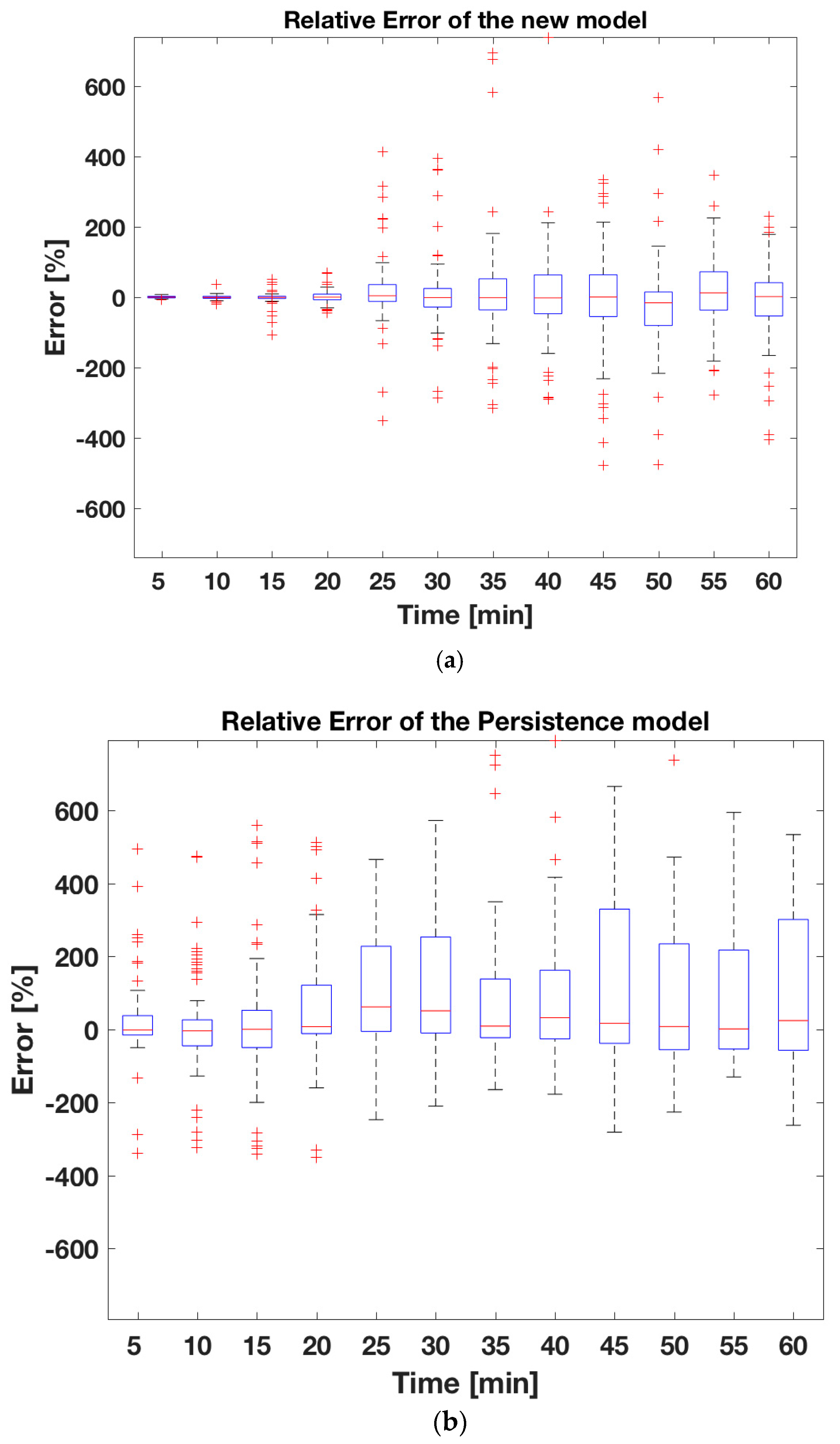
3.3. Analysis of the Statistical Sampling

Figure 6 shows the distribution of the relative deviations as boxplots. The results of Figure 6a suggest that the new model shows a symmetrical approach for 50% of the sample rate for the first several simulation minutes. Nevertheless, Figure 6b shows an asymmetrical distribution of outliers and a decreasing number of outliers for higher sample sizes, leading to higher uncertainties in the simulation of the data. As expected, the uncertainty of the new model decreased as soon as more simulation data were introduced and remained constant with the increase of sample sizes. It is worth noting that in the persistence model, the uncertainty increased as soon as more simulation data were introduced.

In order to estimate how many simulations were needed to carry out the validation of our model, statistical sampling was performed. Over 6 months of validation periods and assuming that we could simulate an average of 8 h every day, we got 1440 valid cases. In these 6 months, 80 cases were not considered because the irradiance level was under 100 W/m². Hence, our final valid cases numbered 1360 and, to validate our algorithm, we applied statistical sampling. Thus, taking into consideration a confidence level of 95% with a margin of error of 6%, our simulated cases numbered 288 (i.e., 288 h). Therefore, each interval time corresponded to one hour of simulation, and from these 288 cases, 96 cases corresponded to cloudless hours, 96 cases to overcast hours, and 96 cases to broken cloud hours. For the new method, if on the horizon the presence of clouds is zero, it is very likely that in the next few minutes, near the sun, there will be no cloud, as well. Thus, for clear sky days, the deviations varied 8% compared to the measurement values. Overcast days and days with broken clouds represented a very important challenge for the neural network. The deviations varied approximately 24% according to the type of clouds and the amount of clouds on the horizon compared to the measurement values. In addition, on days with broken clouds, the deviations varied 32% according to the percentage of clouds and blue sky between the horizon and the center of the sun compared to the measurement values. Applying the new ANN model to the 288 cases, our model achieved an average 22% deviation compared to the measurement values for all sky conditions. In contrast, the persistence model shows a 52% deviation for the three cases.

4. Conclusions

A new method developed to forecast solar irradiance one hour ahead has been presented. This new model combines the advantages of using all-sky images and an LM-ANN. The GHI predicted by the proposed methodology improves the forecast for the total amount of energy one hour ahead by reducing both the RMSE and MAE of the simulation by approximately 40% when compared to the persistence model. Furthermore, we showed here that the new model is capable of reproducing the nonlinear nature of the solar irradiance more reliably than statistical linear models.

According to the simulation results, for the first minutes of simulation, the new algorithm outperforms the persistence model. For irradiation levels under 80–100 W/m², the new algorithm does not accurately predict one hour ahead. However, such low irradiances are usually not relevant for the production of solar energy. Nevertheless, for higher irradiance the new algorithm can predict one hour ahead under diverse weather conditions with an average deviation of 22% within the next hour.

The model presented here has only been tested at IMuK. The neural network may be trained with datasets from other places. To achieve this, only the pictures of the desired place with the respective pyranometer measurements are sufficient. This work could be especially relevant for implementing strategies in decisions for the balance of supply and demand of electricity. Additionally, this study will be of interest for energy markets concerned with mitigating utility cost by acquiring more accurate weather predictions. It may also be important for the estimation of power output and to avoid damage to the electrical grid.

References

1. Hofmann, M.; Riechelmann, S.; Crisosto, C.; Mubarak, R.; Seckmeyer, G. Improved synthesis of global irradiance with one-minute resolution for PV system simulations. Int. J. Photoenergy 2014. [Google Scholar] [CrossRef]
2. Statistiken. 2007. Available online: https://www.volker-quaschning.de/datserv/pv-welt/index.php (accessed on 9 February 2018).
3. Bundesnetzagentur (2013). Available online: https://www.bundesnetzagentur.de/DE/Sachgebiete/ElektrizitaetundGas/Unternehmen_Institutionen/ErneuerbareEnergien/ZahlenDatenInformationen/zahlenunddaten-node.html (accessed on 17 February 2018).
4. Mathiesen, P.; Kleissl, J. Evaluation of numerical weather prediction for intra-day solar forecasting in the continental United States. Sol. Energy 2011, 85, 967–977. [Google Scholar] [CrossRef]
5. Martínez, L.M.; Vargas, M.; Rubio, F.R. Vision-Based System for the Safe Operation of a Solar Power Tower Plant; Springer: Berlin, Germany, 2002. [Google Scholar]
6. Zhen, Z.; Wang, Z.; Wang, F.; Mi, Z.; Li, K. Research on a cloud image forecasting approach for solar power forecasting. Energy Procedia 2017, 142, 362–368. [Google Scholar] [CrossRef]
7. Alonso, M.J.; Batlles, F.J.; Portillo, C. Solar irradiance forecasting at one-minute intervals for different sky conditions using sky camera images. Energy Convers. Manag. 2015, 105, 1166–1177. [Google Scholar] [CrossRef]
8. Marquez, R.; Coimbra, C.F.M. Intra-hour DNI forecasting based on cloud tracking image analysis. Sol. Energy 2013, 91, 327–336. [Google Scholar] [CrossRef]
9. Chu, Y.; Pedro, H.T.C.; Nonnenmacher, L.; Inman, R.H.; Liao, Z.; Coimbra, C.F.M. A Smart image-based cloud detection system for intrahour solar irradiance forecasts. J. Atmos. Ocean. Technol. 2014, 31, 1995–2007. [Google Scholar] [CrossRef]
10. Chi, W.C.; Bryan, U.; Matthew, L.; Anthony, D.; Jan, K.; Janet, S.; Byron, W. Intra-hour forecasting with a total sky imager at the uc san diego solar energy testbed. Sol. Energy 2011, 85, 2881–2893. [Google Scholar]
11. Wu, J.; Keong, C.C. Prediction of hourly solar radiation using a novel hybrid model of arma and tdnn. Sol. Energy 2011, 85, 808–817. [Google Scholar]
12. Kamadinata, J.O.; Tan, L.K.; Tohru, S. Global Solar Radiation Prediction Methodology using Artificial Neural Networks for Photovoltaic Power Generation Systems. Smartgreens 2017. [Google Scholar] [CrossRef]
13. Almeida, M.P.; Perpinán, O.; Navarrete, L. PV power forecast using a nonparametric PV model. Sol. Energy 2015, 115, 354–368. [Google Scholar] [CrossRef] [Green Version]
14. Wilks, D.S. Statistical Methods in the Atmospheric Sciences; Academic Press: Cambridge, MA, USA, 2011. [Google Scholar]
15. Richard, P.; Sergey, K.; James, S.; Karl, H.J.; David, R.; Thomas, E.H. Validation of short and medium term operational solar radiation forecasts in the US. Sol. Energy 2010, 84, 2161–2172. [Google Scholar] [Green Version]
16. Mellit, A.; Kalogirou, S.A. Artificial intelligence techniques for photovoltaic applications: A review. Prog. Energy Combust. Sci. 2008, 34, 547–632. [Google Scholar] [CrossRef]
17. Yang, H.Y.; Ye, H.; Wang, G.Z. Applications of chaos theory to load forecasting in power system. Relay 2005, 33, 26–30. [Google Scholar]
18. Tohsing, K.; Schrempf, M.; Riechelmann, S.; Schilke, H.; Seckmeyer, G. Measuring high-resolution sky luminance distributions with a CCD camera. Appl. Opt. 2013, 52, 1564–1573. [Google Scholar] [CrossRef] [PubMed]
19. Anon. Available online: http://www.kippzonen.com/Product/13/CMP11-Pyranometer#.WXi1sK3qh-U (accessed on 23 May 2018).
20. Yamashita, M.; Yoshimura, M.; Nakashizuka, T. Cloud Cover Estimation using Multitemporal Hemisphere Imageries. Inter. Arch. Photogramm. Remote Sens. Spat. Inf. Sci. 2004, 35, 826–829. [Google Scholar]
21. Schrempf, M. Entwicklung eines Algorithmus zur Wolkenerkennung in Digitalbildern des Himmels. Master’s Thesis, Institut für Meteorologie und Klimatologie, Hanover, Germany, 2012. [Google Scholar]
22. Estimation, F. Full Vectorization of Solar Azimuth and Elevation Estimation-File Exchange-MATLAB Central. Available online: https://de.mathworks.com/matlabcentral/fileexchange/48594-full-vectorization-of-solar azimuth-and-elevation-estimation (accessed on 21 July 2015).
23. Yang, J.; Lu, W.; Ma, Y.; Yao, W. An automated cirrus cloud detection method for a ground-based cloud image. J. Atmos. Ocean. Technol. 2012, 29, 527–537. [Google Scholar] [CrossRef]
24. Liu, S.; Zhang, L.; Zhang, Z.; Wang, C.; Xiao, B. Automatic cloud detection for all-sky images using superpixel segmentation. IEEE Geosci. Remote Sens. Lett. 2015, 12, 354–358. [Google Scholar]
25. Hadja, M.D.; Philippe, L.; Mathieu, D. Solar irradiation forecasting: State-of-the-art and proposition for future developments for small-scale insular grids. In Proceedings of the WREF 2012-World Renewable Energy Forum, Denver, CO, USA, 13–17 May 2012; pp. 1–8. [Google Scholar]
Figure 1. Process of the forecast of the global horizontal irradiance (GHI) with all-sky images and an artificial neural network (ANN).
Energies 11 02906 g001
Figure 2. (a) Original image. (b) Cropped black area of the picture and coverage of the sun. (c) Haze Index image. (d) The picture from the Cloud Locating and Cloud Movement program. In addition, the black contour around the clouds show the possible clouds that could appear over the sun in the next minutes. (e) The picture shows the circles from the center of the sun with uniform distance to the horizon.
Energies 11 02906 g002
Figure 3. Prediction from the reference persistence model for two different days: (a) 18 September 2014 from 14:01 to 15:00. (b) 14 August 2015 from 12:01 to 13:00. The red dots on the lower part of both images indicate the simulated time. The blue dots indicate that the data employed for the simulation was one hour previous to this from the last seven days. The upper part shows a zoom of the simulation day.
Energies 11 02906 g003aEnergies 11 02906 g003b
Figure 4. Comparison of new ANN model and persistence model for one-hour-ahead simulation. The vertical black lines in the graphs represent the border of minutes of future information from the last taken picture. (a) shows a good prediction of the total amount of energy with R2 = 0.92. (b) shows a good prediction especially for the first minutes of simulation. (c) shows a good prediction for the first 32 min of simulation. (d) shows a very important deviation with respect to the measured data; R2 = 38. However, irradiance values of under 80 W/m2 are of minor importance for the overall energy forecast.
Energies 11 02906 g004aEnergies 11 02906 g004b
Figure 5. The hourly average of simulation on 17 July 2015 from 05:01 to 18:00. The grey line shows the measured one-minute values.
Energies 11 02906 g005
Figure 6. The relative deviation boxplot of the simulation derived for different time horizons. The symmetry in 50% of the data decreases as soon as the program receives information from the last picture and increases when the program does not receive information from the last picture. (a) corresponds to the new ANN. Here, there are narrower interquartile ranges for higher sample sizes, but the numbers of outliers (+) are lower than in (b). (b) corresponds to the persistence model. Of the data, 50% is not exactly located in the middle, and the 25% and 75% levels of the data deviation are higher than in (a).
Energies 11 02906 g006