Short-Term Load Interval Prediction Using a Deep Belief Network

Abstract

In load predication, point-based forecasting methods have been widely applied. However, uncertainties arising in load predication bring significant challenges for such methods. This therefore drives the development of new methods amongst which interval predication is one of the most effective. In this study, a deep belief network-based lower–upper bound estimation (LUBE) approach is proposed, and a genetic algorithm is applied to reinforce the search ability of the LUBE method, instead of simulated an annealing algorithm. The approach is applied to the short-term load prediction on some realistic electricity load data. To demonstrate the effectiveness and efficiency of the proposed method, it is compared with three state-of-the-art methods. Experimental results show that the proposed approach can significantly improve the predication accuracy.

1. Introduction

Load prediction plays an important role in the planning of power systems, building reliable power systems and so on. In general there are four types of load predication, that is, long-term, medium-term, short-term, and ultra-short-term forecasting. The short-term load prediction (STLP) is crucially important on the daily operation and scheduling of power systems such as economical dispatching and optimal unit commitment.

To date, there has been a number of studies proposed for STLP. These methods can be loosely categorized as point predication and interval prediction. Representative point predication-based methods include the following: (i) methods based on statistical models, such as state space model [1], regression analysis model [2], autoregressive integrated moving average (ARIMA) [3], Kalman filtering [4], and exponential smoothing (ES) models [5]; (ii) artificial intelligence-based methods, e.g., neural networks (NNs) [6], expert systems [7], support vector machines (SVM) [8], deep learning [9]; and (iii) hybrid models such as neuro-fuzzy systems [10]. However, the main issue of point predication is that it only provides a single value as an output without considering the accuracy or reliability of the predication [11]. Given the increasing uncertainties of the power grid caused by self-powered users and independent microgrids (based on renewable energies) [12], point predication-based methods now face great challenges.

Interval predication-based methods, as the name says, output an interval as the predication results to cover the future observations with a certain confidence level of expectation probability, which is more suitable to deal with uncertainties [13,14]. The upper and lower bounds in interval predication can not only highly cover the fallen objectives, but they also provide an accurate coverage probability as an indication, which obviously brings more quantitative information than point prediction.

Table 1. The features of four traditional neural network (NN)-based predication interval (PI) construction methods [15].

Method	Advantage	Disadvantage
Delta method	NN is enhanced by the nonlinear regression technique	The use of linearization in NN
Bayesian method	Strong theoretical foundation of Bayesian concepts	Large computational burden required for the calculation of a Hessian matrix
Bootstrap method	Ease of implementation	The need of a large data set to support training and calculation
Mean-variance estimation-based method	The low calculation cost of the training process	The low empirical coverage probability

listed several representative interval predication methods. The delta method adopts a nonlinear regression technique to enhance the generalization performance of the neural network (NN) models [15]. First, the method linearized the neural network model by a set of parameters generated by minimizing the sum of the squared error cost functions. Then, the linearization model applied the standard asymptotic theory to construct predication intervals (PIs) [16]. The main issue of the above method is the use of the linearization that simplifies the approach but that may lose effect when the dataset shows strong non-linearity. Bayesian techniques are used to train neural networks, and they allow the predicted value to have a certain error range [17]. However, the need to calculate the Hessian matrix of the cost function constructed makes the calculation of this method expensive. The Bootstrap method is perhaps the most widely used technique for NN-based interval predication, due to its simplicity and ease of implementation [18]. Compared with the aforementioned methods, the Bootstrap method does not need to calculate the derivative and the Hessian matrix. However, it requires a large data set to support the training process. The mean-variance estimation-based method can enhance the ability of the NN model to estimate the distribution characteristics of conditional objectives [19]. The most striking feature of this approach is that it greatly reduces the calculation cost of the training process. However, the low empirical coverage probability is the biggest drawback of this approach.

In addition to the above methods, an alternative interval predication method, namely, the lower upper bound estimation (LUBE), is proposed in 2011 [20]. Compared to existing NN-based interval predication methods, the LUBE does not make any assumption about the distribution of the training data sets or the prediction errors. Also, it avoids mass computational calculation of complex derivatives. In this study a single-objective LUBE framework is adopted, though its multi-objective framework has also been proposed [21,22].

The NN-based LUBE approach has many demonstrated applications [23,24,25]; however, the traditional NN model has its own limitations such as the requirement for a long training time for good performance, and the ease of the model to be trapped in local optima. These limitations have greatly restricted the performance of the NN-based LUBE method. The deep belief network (DBN) has attracted a great deal of attention in the last decade [26]. The DBN adopts a layer-by-layer training method, by which the whole network can be effectively trained. One notable feature of DBN is that it can hierarchically display multiple characteristics of the patterns of data.

In the last decade, there is a growing appeal for using DBN to predict time series data [27]. For example, an empirical mode decomposition (EMD) algorithm is incorporated into DBN to improve the algorithm performance [28]. The particle swarm optimization (PSO) approach was introduced to enhance the learning and extraction capability of the restricted Boltzmann machine (RBM) in DBN [29]. In [30] an adaptive DBN learning architecture is proposed to autonomously generate/eliminate RBM neurons based on the training data patterns. A fast meta-heuristic algorithm was applied to make the parameter settings of DBN more suitable and accurate [31]. The nearest neighbor classification algorithm was combined with the dynamic time warping (DTW) method to obtain first-class prediction performance [32].

In the study, a single-objective framework LUBE method using the DBN is proposed to perform short-term load predication. In addition, a genetic algorithm is applied to reinforce the search ability of the LUBE method, instead of a simulated annealing algorithm. The rest of the paper is organized as follows. Section 2 introduces the background knowledge related to the deep belief network model and the LUBE method; Section 3 elaborates the proposed novel interval prediction framework combing DBN and LUBE; experimental setup, results, and discussions are presented in Section 4; Section 5 concludes the paper and identifies some future directions.

2. Background

This section introduces some necessary background knowledge i.e., the evaluation metrics of the interval predication and the LUBE method.

2.1. Evaluation Metrics of Interval Prediction

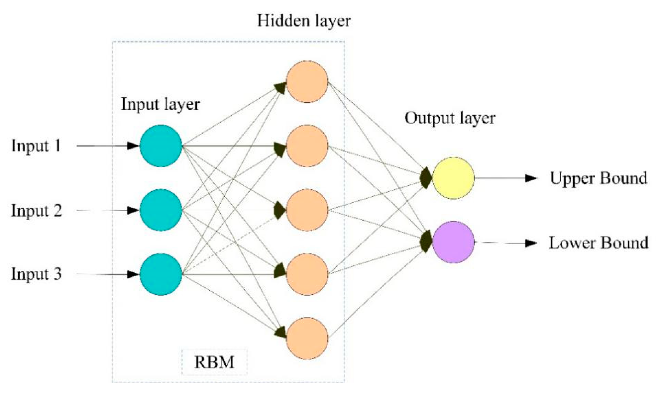
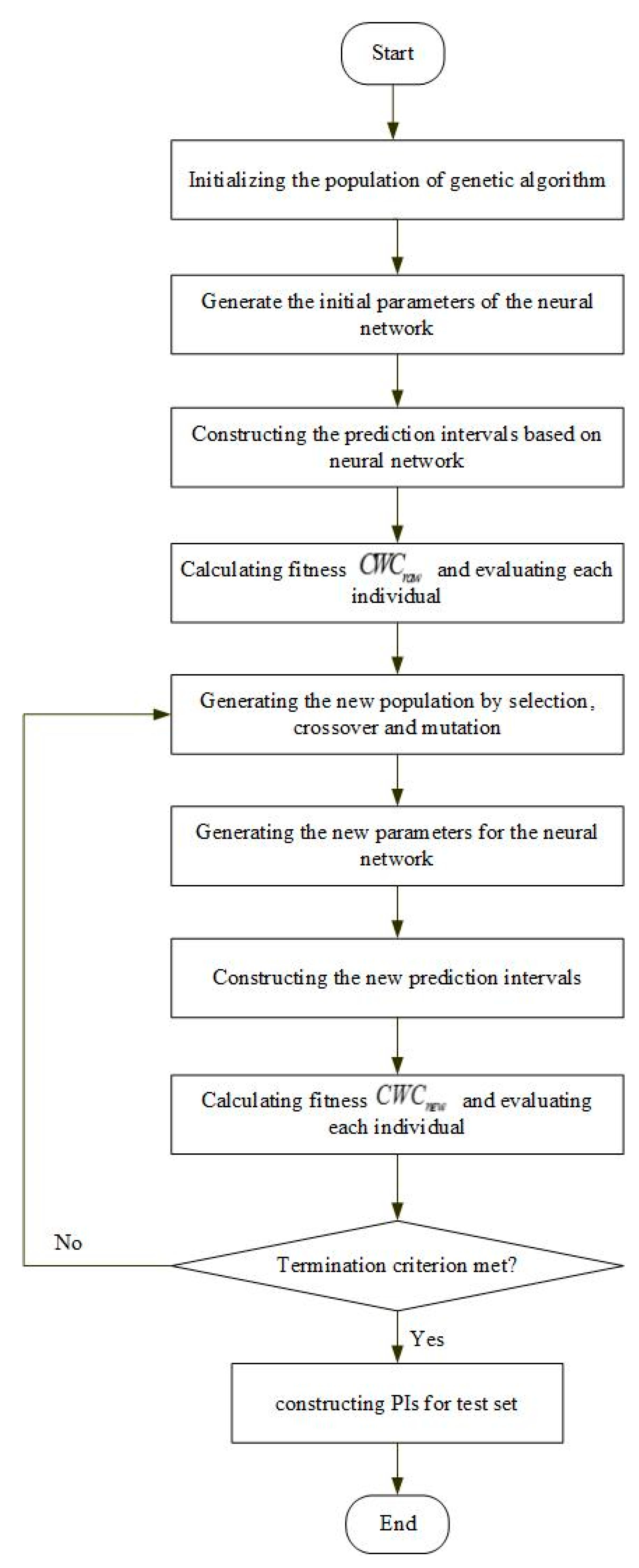
As is well known, the mean absolute percentage error (MAPE) and the mean square error (MSE) are two widely used metrics in point prediction. Likewise, the PI coverage probability (PICP) and the PI-normalized average width (PINAW) are two important metrics in interval predication. Notably, the metrics have to be optimized simultaneously so as to obtain an interval with narrow range but good coverage (i.e., reliability).

Specifically, the PICP measures the number of objective values that are within the predicted interval. The larger the PICP, the better the predication results. Mathematically, the PICP can be defined as follows:

$$\mathrm{PICP}=\frac{1}{n}{\displaystyle \sum _{i=1}^n{c}_i}$$

(1)

where $n$ denotes the number of objective sets, and $c_i$ is a Boolean variable defined by:

$$c_i=\{\begin{array}{l}1,if{y}_i\in \left[L_i,U_i\right];\\ 0,if{y}_i\notin \left[L_i,U_i\right].\end{array}$$

(2)

The variable $c_i$ describes the coverage degree of predicated interval (PI). If the objective value $y_i$ lies within the lower bound $L_i$ and the upper bound $U_i$, then $c_i=1$; Otherwise, $c_i=0$. The ideal case, $\mathrm{PICP}=100\%$, indicates that all objective values are within the predication interval.

A little more thought can reveal that a sufficiently wide PI would result in $\mathrm{PICP}=100\%$. However, this is obviously not applicable. Therefore, another metric has to be introduced, the PINAW, which is expect to be minimized; see Equation (3):

$$\mathrm{PINAW}=\frac{1}{N\cdot S}{\displaystyle \sum _{i=1}^N\left(U\left(X_i\right)-L\left(X_i\right)\right)}$$

(3)

where $S$ measures the range of the objective values, i.e., the maximum objective value minus the minimum. It is used to standardize the average width of the PI as a percentage. In this way, PINAW can be applied to quantitatively examine the performance of the constructed PI by different methods.

Obviously, the PICP and PINAW are in conflict with one another. A narrow interval (a small PINAW) has a large probability to result in a small PICP. Thus, to assess the overall performance of the interval predication methods, a comprehensive cost function is required to consider both the coverage probability and the width of the predication interval. Moreover, as PICP is the basic feature of interval predication methods, the proposed cost function is designed to give more weight to the variation of PICP. In short, the coverage width-based criterion (CWC) is as follows:

$$\mathrm{CWC}=\mathrm{PINAW}+\gamma \left(\mathrm{PICP}\right)e^{-\eta \left(\mathrm{PICP}-\mu \right)}$$

(4)

where $\gamma \left(\mathrm{PICP}\right)$ is a Boolean function:

$$\gamma =\{\begin{array}{l}1,if\mathrm{PICP}<\mu ;\\ 0,if\mathrm{PICP}\ge \mu .\end{array}$$

(5)

where $\eta$ is used to penalize the invalid PI, while $\mu$ can be determined by the confidence level of PI.

2.2. LUBE Approach

Different from traditional interval predication methods, the LUBE approach directly approximates the upper and lower bounds of the PI by unsupervised learning methods. As is mentioned in the last section, the LUBE aims to achieve a narrow predication interval and a high coverage probability of objective values, which is a typical bi-objective optimization problem. By Equation (4), the bi-objective problem is reasonably transformed into a single-objective problem, minimizing the unified indicator, CWC.

The proposed metric, CWC, is therefore used to train an NN, so as to construct PI. The NN model has two outputs, the upper bound and the lower bound. A genetic algorithm is applied to reinforce the search ability of the LUBE method. Figure 1 illustrates a typical flowchart of the NN-based LUBE approach. The main steps are described as follows.

Step 1

Population initialization: randomly initialize the population of the genetic algorithm (GA). The weights and thresholds of the NN models are generated based on the population.

Step 2

PI construction and ${\mathrm{CWC}}_{raw}$ calculation: an NN with two outputs is applied to construct PIs for the training data. PICP, PINAW, and CWC are then calculated, which are taken as the initial fitness of the genetic algorithm.

Step 3

Generation of a new population: the selection, crossover, and mutation operators are performed on the parent population to produce new offspring.

Step 4

PIs construction: a new PI is constructed by using new selected NN parameters. Accordingly, the new metric ${\mathrm{CWC}}_{new}$ is calculated by Equation (4).

Step 5

Each individual evaluation: The index CWC is considered as the fitness in the GA optimal process. The individual with the minimum fitness is recorded as the global optimal solution. The individual also represents the best model parameters.

Step 6

Termination and Results: usually there are frequently used termination criteria, i.e., the maximum number of iterations is reached, or the evaluation indicator remains unchanged for a number of interactions. If the criteria is not met, then the algorithm returns to Step 3.

3. Single-Objective LUBE Framework for DBN-Based Interval Predication

As mentioned previously, the LUBE method directly constructs a predication interval. This is of low computational cost, and it is easy to implement. At present, most studies are based on a NN model to build prediction intervals. However, compared with the NN model, a DBN with RBM structure can discover inherent features of data which is therefore more suitable in predicting time series data. This section thus elaborates the use of DBN-based model for interval prediction.

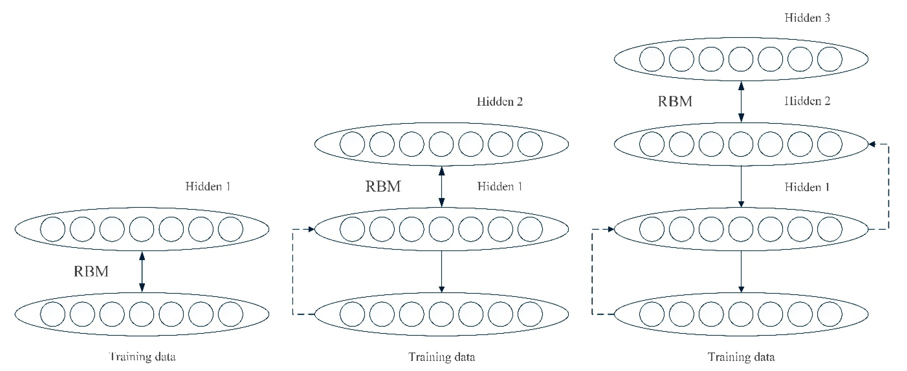
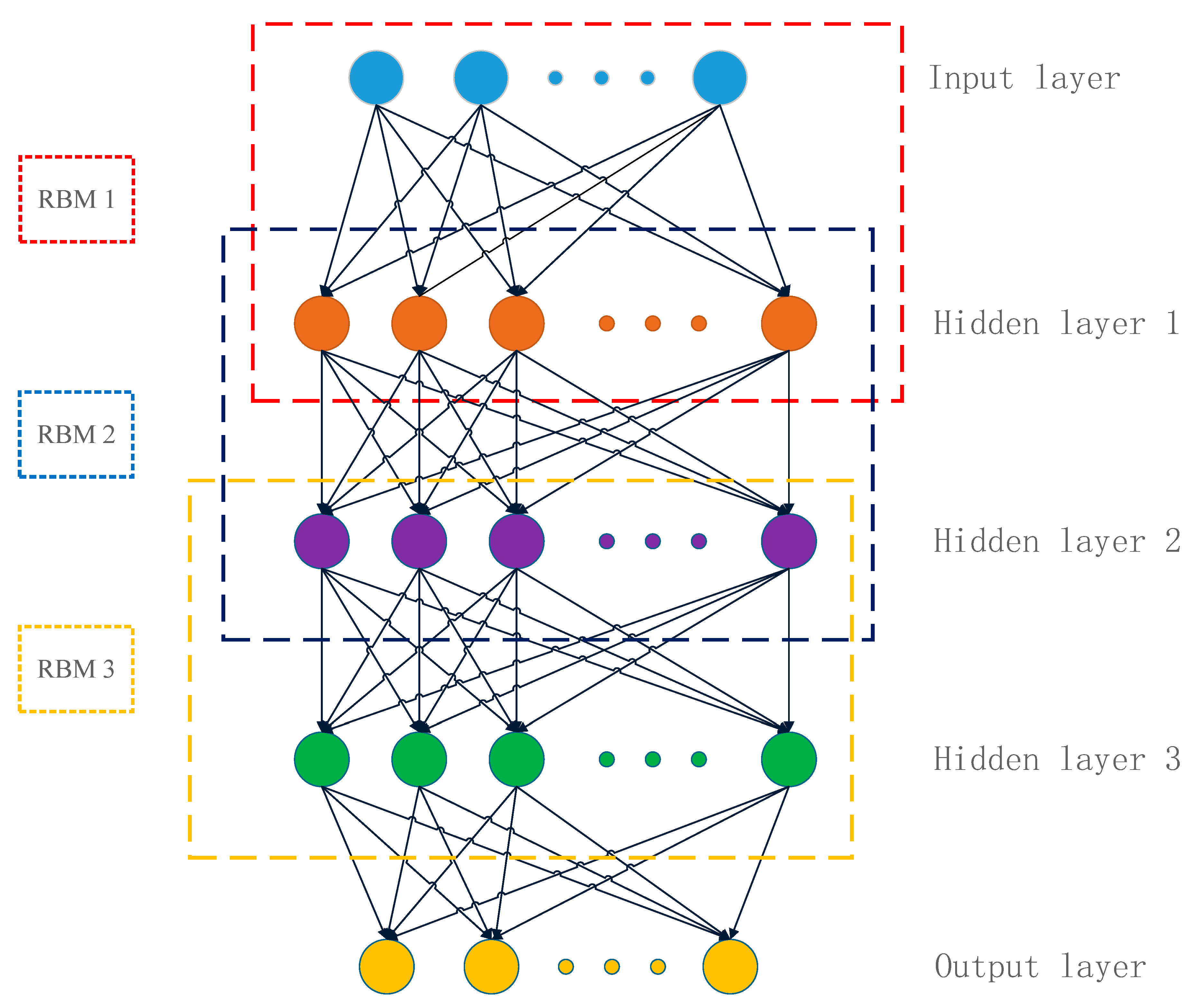
3.1. Deep Belief Network Model

The DBN model generally consists of several restricted Boltzmann machines (RBM), stacking, and a layer of NN [33]. The training process of DBN contains two phases: a layer-wise pre-training process and a fine-tuning process. The former provides better initial values of the network parameters, and the latter searches optimal parameters of the network. A typical DBN is illustrated in Figure 2.

3.1.1. Pre-Training Process

The goal of the pre-training process is to generate a good set of network parameters for the DBN model. The configuration of parameters is obtained through an unsupervised greedy optimization algorithm by using the (RBM).

RBM, a stochastic binary structure, can learn the distribution characteristics of sample data [34,35]. This binary structure consists of visible layers and hidden layers. There are connections between the visible layer and the hidden layer, while there is no connection within the layer. These connections are bidirectional and symmetrical. Figure 3 shows the typical structure of RBM.

The RBM is an energy-based model. The energy of the joint configuration of the visible and hidden layers can be expressed as below:

$$E\left(v,h\right)=-{\displaystyle \sum _i{\displaystyle \sum _j{w}_{ij}{h}_i{v}_j}}-{\displaystyle \sum _i{b}_i{h}_i}-{\displaystyle \sum _j{a}_j{v}_j}$$

(6)

where $h_i$ represents the state of the hidden layer unit $i$, and $v_j$ represents the state of the visible layer unit $j$. $w_{ij}$ is the weight between the units. $b_i$ and $a_j$ represent the thresholds of the units. The energy function is applied to calculate the probability that is assigned to each pair of visible and hidden vectors. The lower the energy, the closer the network is to the desired goal. The probability distribution between the visible layer and the hidden layer is defined as follows:

$$p\left(v,h\right)=\frac{1}{M}{e}^{-E\left(v,h\right)}$$

(7)

where $M$ is a partition function that counts $e^{-E\left(v,h\right)}$ over all possible configurations, and regularizes it as below:

$$M={\displaystyle \sum _{v,h}{e}^{-E\left(v,h\right)}}$$

(8)

Given the activation unit of the visible layer, the activation probability of the hidden layer unit is:

$$p_{h_i}=p\left(H_i=1|v\right)=\sigma \left({\displaystyle \sum _j{w}_{ij}{v}_j}+b_i\right)$$

(9)

where $\sigma$ is the logistic sigmoid function:

$$\sigma \left(x\right)=\frac{1}{\left(1+\exp \left(-x\right)\right)}$$

(10)

Accordingly, for a given hidden unit vector, the state probability of the visible layer specific unit can be expressed as:

$$p_{v_j}=p\left(V_j=1|h\right)=\sigma \left({\displaystyle \sum _i{w}_{ij}{h}_i}+a_j\right)$$

(11)

The update process of the RBM is described below. The number of units selected for the visible layer is the same as the number of training data given, and then Equation (10) is used to calculate the state of the corresponding hidden layer. Similarly, based on the state obtained by the hidden layer unit, the state of the visible layer unit is calculated by Equation (11). After a number of such loops, the resulting unit is denoted as $h_i{}^{\prime }$ and $v_j{}^{\prime }$. Related parameters of RBM are updated as follows:

$$\Delta b_i=\eta \left(\langle h_i\rangle -\langle h_i{}^{\prime }\rangle \right)$$

(12)

$$\Delta a_j=\eta \left(\langle v_j\rangle -\langle v_j{}^{\prime }\rangle \right)$$

(13)

$$\Delta w_{ij}=\eta \left(\langle v_j{h}_i\rangle -\langle v_j{}^{\prime }{h}_i{}^{\prime }\rangle \right)$$

(14)

where $\langle \cdot \rangle$ epresents the expectation of training data, and $\eta$ refers to the learning rate.

3.1.2. Fine-Tuning Process

After the pre-training, the DBN network adjusts its connection weights by the back propagation (BP) algorithm. This process is called fine-tuning, which enables the DBN to have better discriminant performance. Based on the loss function of the network, a gradient descent algorithm is adopted to adjust the network parameters, wherein the loss function defined in Equation (15) is applied to find the optimal parameter setting:

$$L\left(y,y^{\prime }\right)={\Vert y-y^{\prime }\Vert }_2^2$$

(15)

where $y^{\prime }$ defines the forecast point and $y$ defines the actual point.

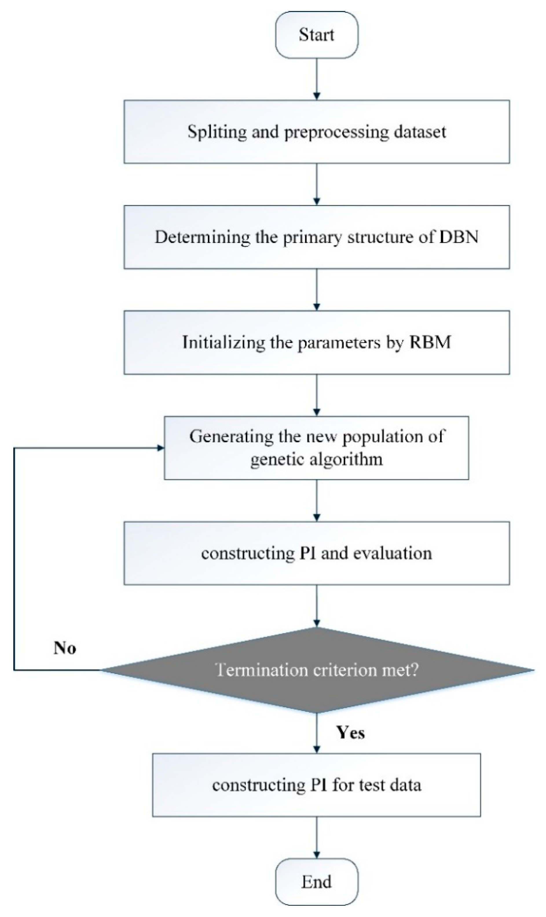
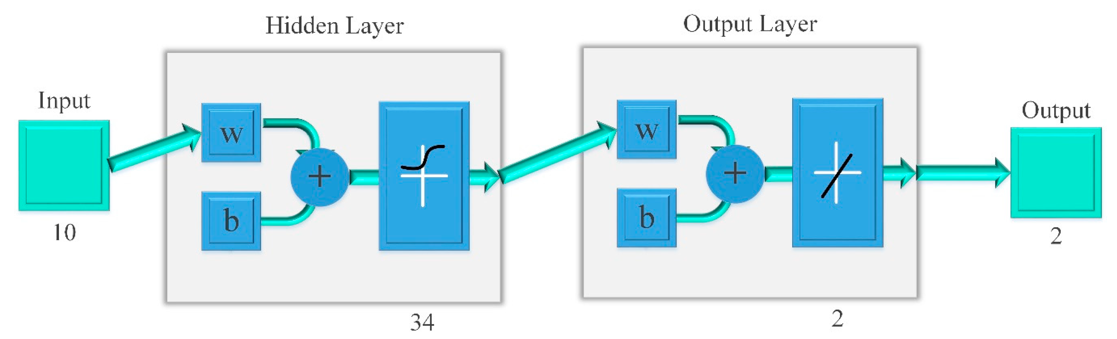
3.2. Model Implementation

Based on the DBN model and the LUBE method, the predication interval can be constructed, and the schematic diagram is shown in Figure 4. Moreover, Figure 5 shows the flowchart of the DBN-based LUBE method. The main steps are discussed below.

Step 1

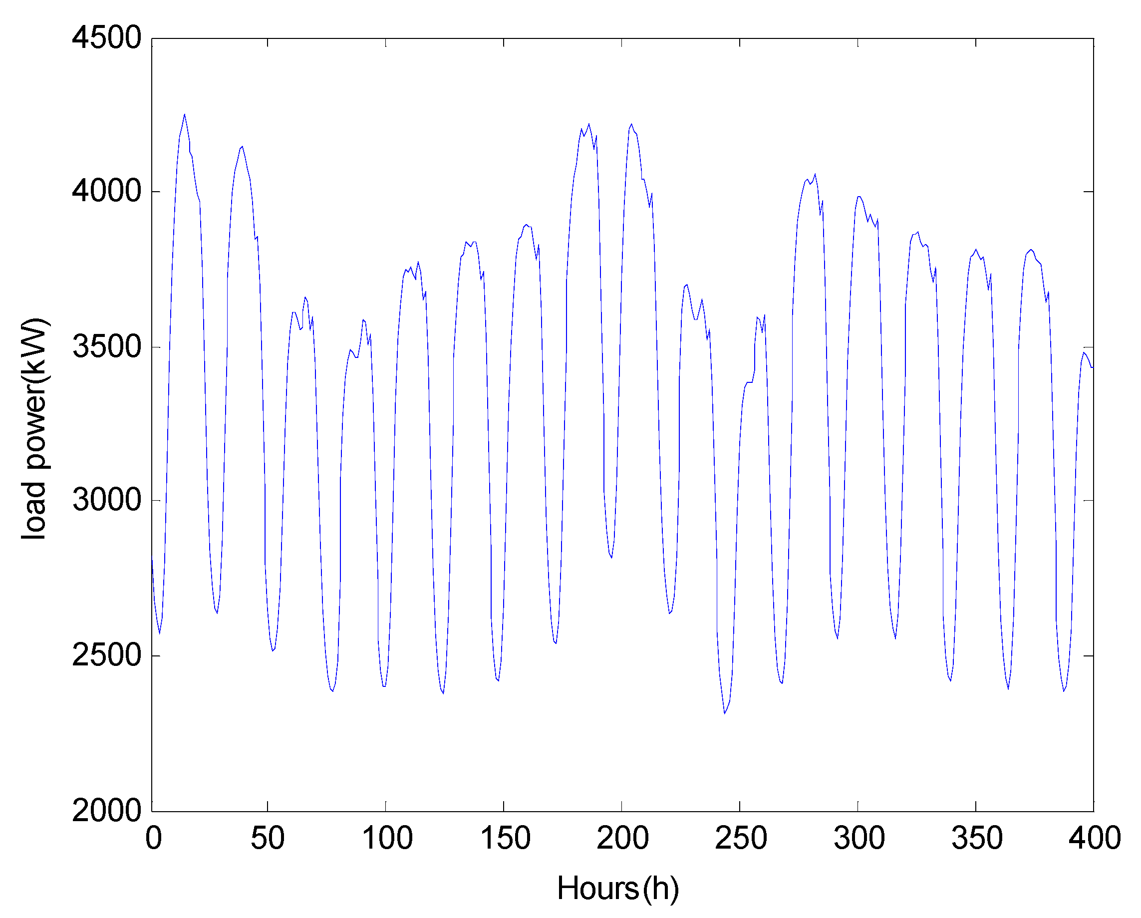
Data processing. As is known, the power system is a typical nonlinear system, which is affected by various natural and social complex factors. In order to establish an accurate prediction model, the load forecasting method needs to quantify the effects of various factors, but such quantification is often very difficult. Since the evolution of any component of the system is determined by the other components that interact with that component, the load time series contains the long-term evolution information of all variables that affect the load. Therefore, studying the regularity of load and predicting the future development trend of load power can only use historical load data. The theoretical basis of this prediction method is the phase space reconstruction theory proposed by Packard et al. [36].

Assuming that the time series of a component of the system is observed as $\left\{x\left(k\right),k=1,2,\cdots ，N\right\}$, then a point state vector reconstructed in the phase space can be expressed as:

$$X\left(i\right)=\left[x\left(i\right),x\left(i+\tau \right),\cdots ,x\left(i+\left(m-1\right)\tau \right)\right],i=1,2,\cdots ,M$$

(16)

where $M$ is the number of phase points in the reconstructed phase space, $M=N-\left(m-1\right)\times \tau$. $m$ and $\tau$ respectively represent the embedding dimension and the time delay of the system.

The authors in [37] demonstrated that when the embedding dimension is sufficiently large, the reconstruction algorithm is an embedded mapping. The reconstructed phase space can preserve many characteristics of the dynamic system, and can recover the dynamic characteristics of the system in the sense of topological equivalence.

The key point of the phase space reconstruction technology is to correctly select the embedding dimension $m$ and the time delay $\tau$. A small $m$ cannot show the real structure of a complex system, while a large $m$ makes the true structural relationship between the points unclear, due to the decrease of the density of the points. Therefore, it is necessary to select an appropriate embedding dimension, $m$. In practical applications, due to the limited data, the choice of an appropriate $\tau$ is also critical. If $\tau$ is too small, the correlation of the coordinates is too strong, so that the information is not easily revealed; if $\tau$ is too large, the power system will be distorted. Overall, in this study, the two parameters are determined by the mutual information function and the false nearest neighbor method.

Once the time delay and embedding dimension are determined, the time series can be reconstructed. Then it can be applied to train the DBN model. In this case, the number of input units of the model is equal to the embedding dimension.

Step 2

Determine the primary structure of DBN. In this study, the trial and error method is used to find the appropriate number of hidden units in the DBN model. The number of input units is determined by the delay time.

Step 3

Parameter initialization. The parameters of DBN model are initialized by the RBM using Equations (12)–(14).

Step 4

Generation of new population of GA. The new population is used to update the weights and thresholds of DBN, and then we can obtain new cost function. A smaller cost function value in this study will be retained.

Step 5

Model evaluation. First, predication intervals are constructed by the DBN model, then the corresponding metrics, i.e., PICP and PINAW, are calculated. Finally, CWC (a combination of PICP and PINAW) is used to evaluate the quality of the PI.

Step 6

Termination criterion. If the termination condition is met, then the training is terminated. Otherwise return to step 3.

Step 7

Construct PI. Construct the predicated intervals by the obtained optimal DBN model.

4. Experiment

In this section, we describe the historical power load data of a small town in the UK as the short-term load forecasting case. To demonstrate the prediction performance of the proposed model, the proposed method is compared against three other state-of-the-art models.

4.1. Preprocessing of Data Set

The entire dataset uses real-world electricity load data of a small town in the UK in 2013, which is a 24 h daily load data from 1 January 2013 to 31 December 2013. According to the LUBE method, the data set needs to be divided into two parts: the training set and the test set. In this paper, we chose nearly 75% of the data set (i.e., the first 273 days) as the training set, and the remaining data (i.e., the last 92 days) as the test set to evaluate the predictive performance of the DBN-LUBE model. The power load data for the entire month of August 2013 is shown as an instance in Figure 6.

4.2. Parameter Settings

Before constructing the prediction interval, we needed to determine the number of input units and hidden units of the DBN model. The number of input nodes is related to the embedding dimension, which can be determined by the phase space reconstruction theory. By the mutual function and the false nearest function in the TISEAN toolbox [38], $m$ is calculated as 10, and $\tau$ is 6. In this case, the dimension of reconstructed delay vectors is 10 and the number of input units for the DBN model is also 10. Specifically, the selection of training sample and training objective is shown in

Table 2. Training sample and training objective.

Training Sample	Training Objective
$x_1,x_7,x_{13},\cdots ,x_{55}$	$x_{56}$
$x_2,x_8,x_{14},\cdots ,x_{56}$	$x_{57}$
…	…
$x_{6500},x_{6506},x_{6512},\cdots ,x_{6554}$	$x_{6555}$

.

The number of hidden units was obtained by the trial and error method. The trial and error results of the DBN model are illustrated in Figure 7. It can be observed from the figure that the MSE achieved optimal performance when the number of hidden units was 34.

Therefore, the optimal structure of the DBN used in this case was 10-34-2. The diagram of the model is illustrated in Figure 8. For the DBN model, the transfer functions of the output neurons and the hidden neurons were the pure linear and tan-sigmoid functions, respectively.

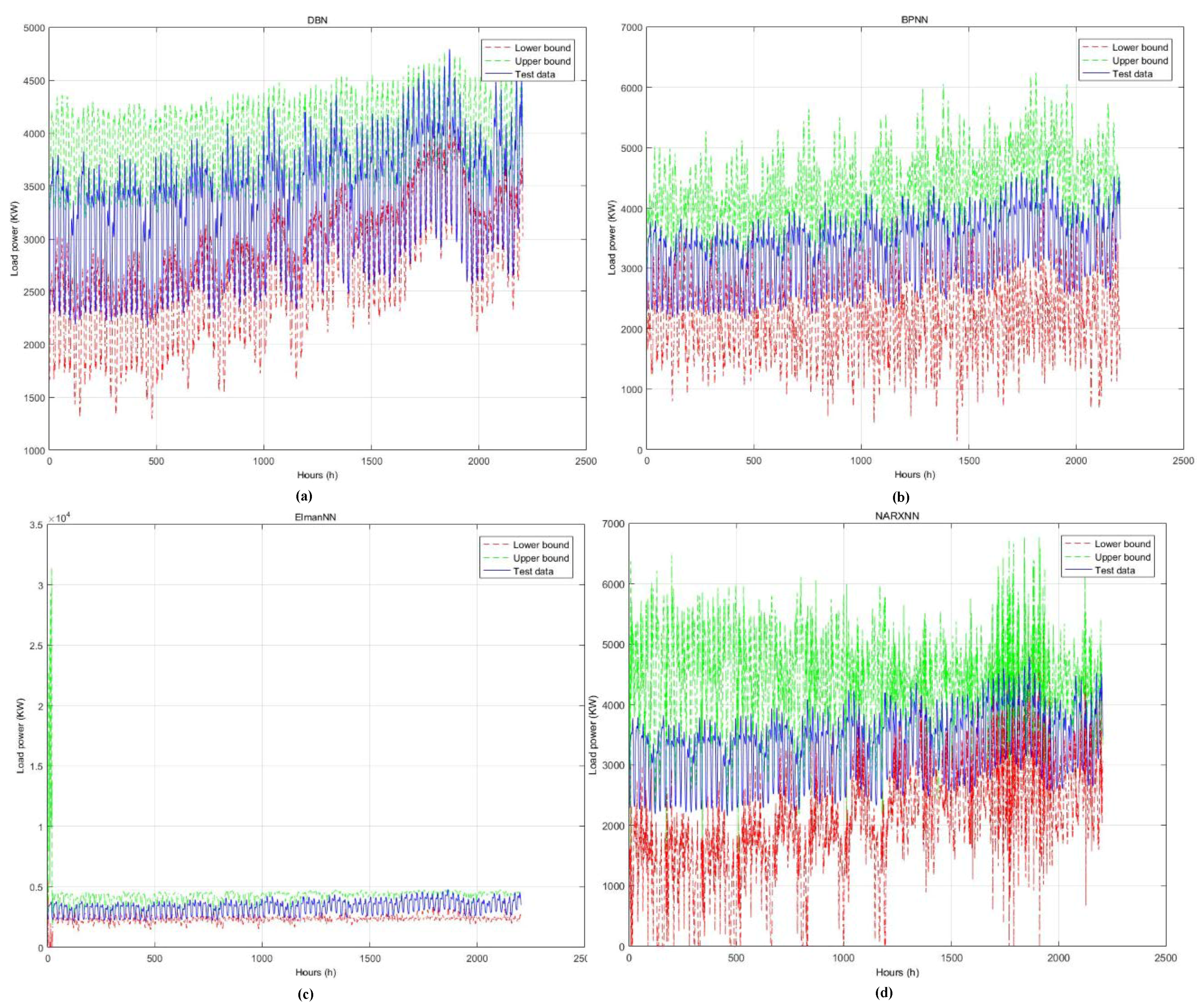
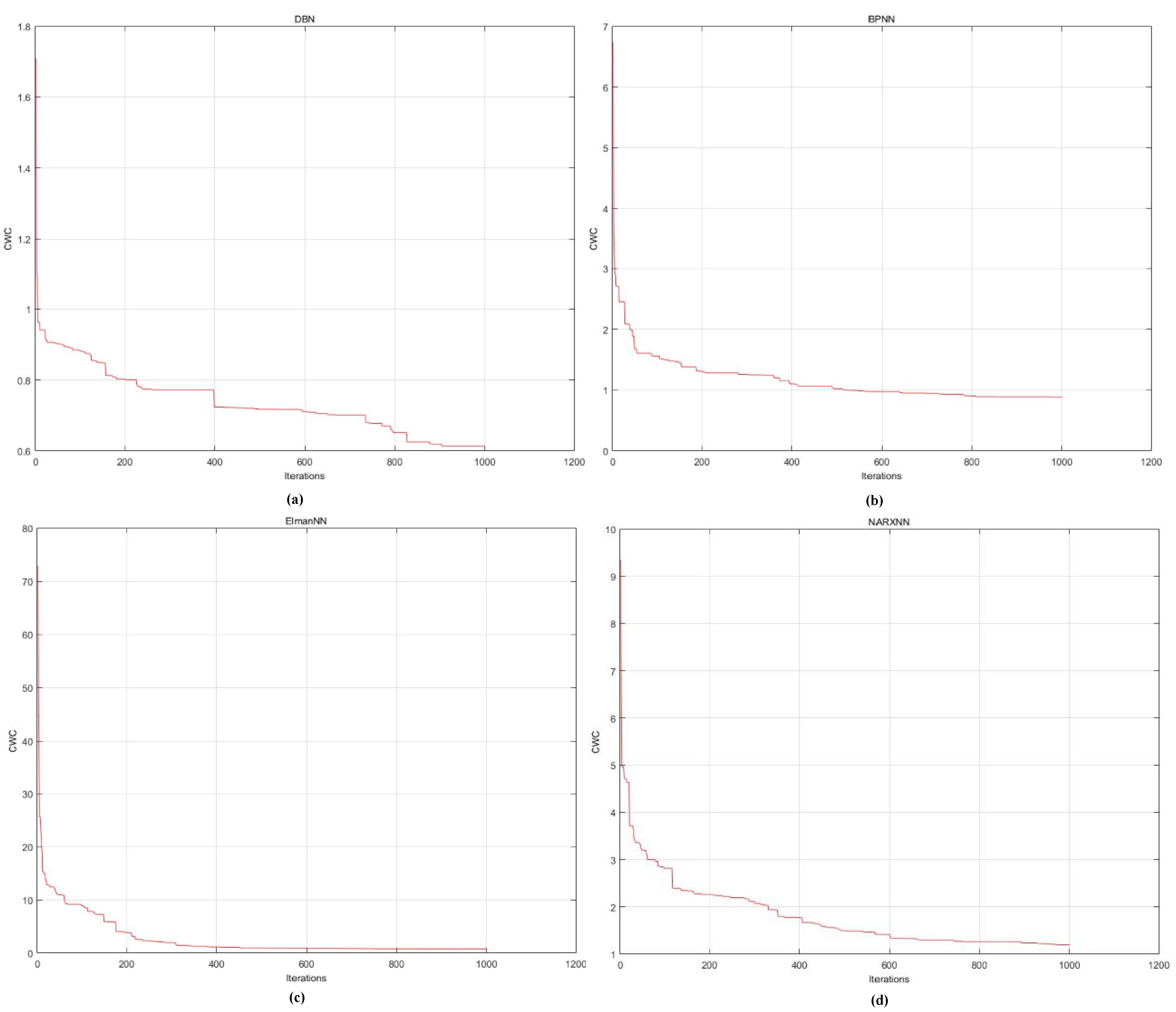
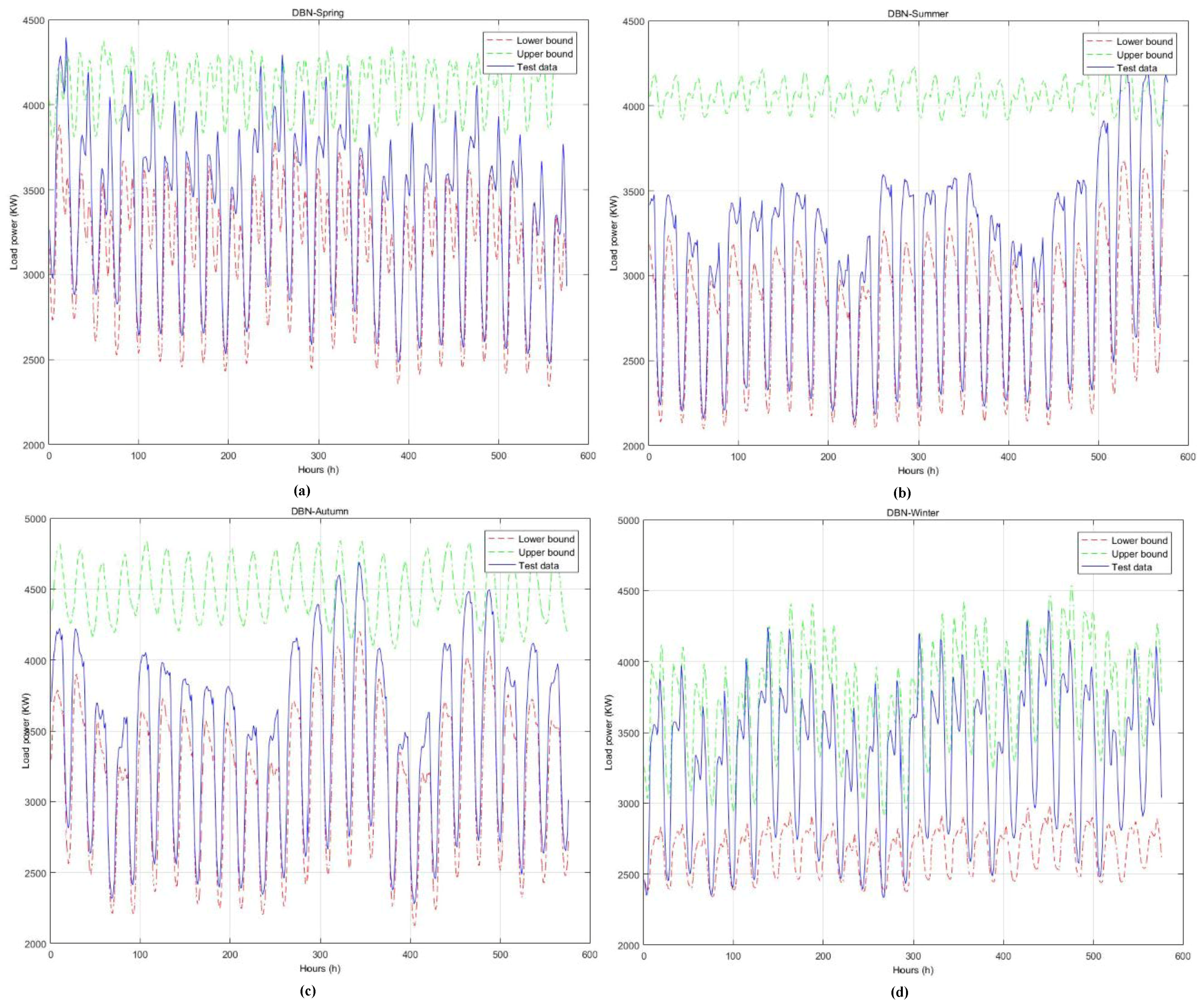
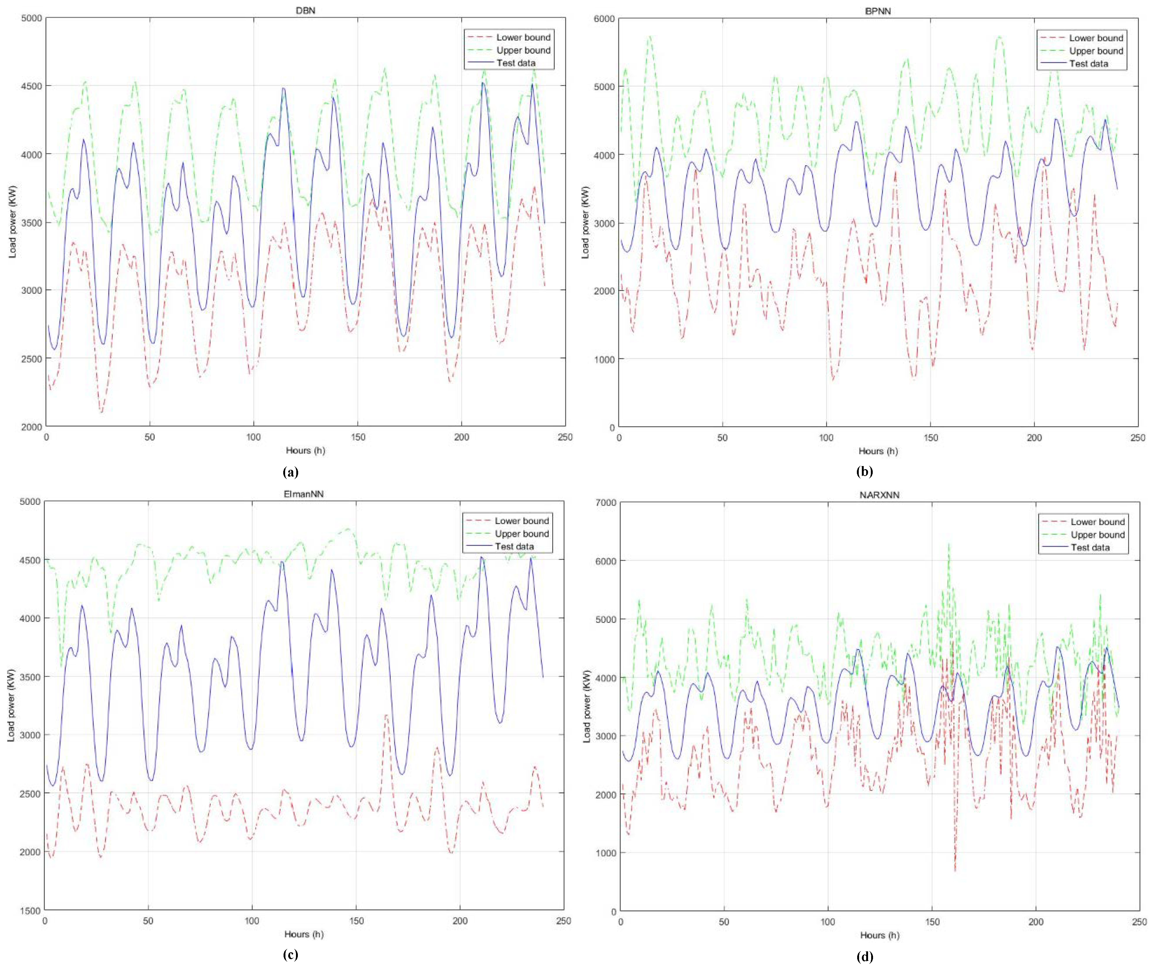
4.3. Results Analysis

In the experiment, the proposed DBN-based LUBE method was compared with three best-in-class prediction models, i.e., the Elman model [39], the nonlinear autoregressive exogenous (NARX) model [40], and the back propagation (BP) network neural model [41].

The comparative prediction results obtained by the four forecasting models for the entire test data are shown in Figure 9. In Figure 9, the prediction results by the DBN fell within the range of the 1300‒4800 KW load, which was the narrowest width of the constructed PIs. Compared to the DBN model, in the BP and NARX models, the predicted intervals were a bit wider. Although most of the predictions of the Elman model were good, the prediction range of the model at the beginning was too volatile, exceeding by an order of magnitude.

In order to better show the comparative test results, we selected the results of the four prediction models for the same 10 continuous days, which are respectively shown in Figure 10. In Figure 10, the construction PI of DBN model can perfectly cover the test data. The prediction results by the Elman model also cover most of the test data, but the PI is much wider than that of DBN. Compared to the DBN model, the reliability of the prediction results by the BP and NARX models were much worse. From the results, it can be concluded that the proposed method provided a narrower width and better reliability.

In

Table 3. Comparative results of the four models in terms of different indicators.

Model	CWC (%)	PICP (%)	PINAW (%)	Time
DBN	47.02	96.60	47.02	578.41 s
BP	81.84	95.83	81.84	629.97 s
Elman	79.45	96.42	79.45	982.52 s
NARX	91.16	91.38	91.16	970.92 s

, the prediction results are compared in terms of four indicators. The CWC indicator is the overall evaluation indicator. According to Equation (4), the smaller the CWC, the better the prediction performance. From Table 3, the CWC of the DBN-based LUBE approach was 0.4702, which was the best. Moreover, in terms of the PI coverage probability, DBN model showed significant superiority over the Elman model. The DBN was also much better than the BP neural network model for the PI-normalized average width. Besides, the DBN model had the shortest running time.

During the iteration, the change of the optimum individual’s fitness by the four models is depicted in Figure 11. In Figure 11, the CWC indicator of all models decreased sharply and achieved satisfactory results in the initial iterations. As the search progressed, the CWC indicator continued to decrease and eventually it converged to the optimal value. The convergence performance shows that the network model with RBM-initialized network weights had stronger optimization capabilities. Compared with the optimal results, the initial and optimal fitness of the DBN model were significantly superior to the results of other models.

To demonstrate the superiority of the proposed method even further, Figure 12 and

Table 4. Prediction results on four seasons.

Season	CWC (%)	PICP (%)	PINAW (%)	Time
Spring	51.08	96.01	51.08	153.46 s
Summer	57.74	96.01	57.74	158.88 s
Autumn	54.94	99.83	54.94	157.53 s
Winter	54.47	93.75	54.47	164.43 s

show the construction PI of the DBN model over four seasons. Overall, the DBN model had a great prediction performance for all the four seasons. Comparing the prediction results of the four seasons, the summer results were the worst. The reason might be that the temperature in summer changes more significantly than in the other seasons.

5. Conclusions

Load prediction often involves a number of uncertainties which makes point predication-based methods not applicable in practice. Interval prediction, as an effective method to quantify uncertainties, therefore has attracted more and more attention. In this study, a selection of point and interval predication methods are first briefly reviewed, then a DBN-based lower upper bound estimation (LUBE) method for short-term load interval forecasting is proposed. To demonstrate the superiority of the proposed method, we compare the DBN-based LUBE method with three state-of-the-art methods, i.e., the BP neural network, the Elman neural network and the NARX neural network. Experimental results show that the DBN-based LUBE method provides the best predication results in a relatively short period of time.

In terms of future work, more empirical tests should first be performed to further demonstrate the effectiveness of the proposed method. Second, in the single-objective LUBE method, the final objective function CWC is a simple combination of PICP and PINAW, and the forecast accuracy and robustness are generally two conflicting objectives; thus, a multi-objective prediction method should be further studied. Lastly, future studies should also consider the potential effects of an advanced evolutionary algorithm [42,43,44] to enhance the performance and efficiency of the multi-objective method.

References

1. Patterson, T.A.; Thomas, L.; Wilcox, C.; Ovaskainen, O.; Matthiopoulos, J. State–space models of individual animal movement. Trends Ecol. Evol. 2008, 23, 87–94. [Google Scholar] [CrossRef] [PubMed]
2. Hayes, A.F. Introduction to Mediation, Moderation, and Conditional Process Analysis: A Regression-Based Approach; The Guilford Press: New York, NY, USA, 2014. [Google Scholar]
3. Li, W.; Zhang, Z. Based on time sequence of ARIMA model in the application of short-term electricity load forecasting. In Proceedings of the 2009 International Conference on Research Challenges in Computer Science, Shanghai, China, 28–29 December 2009. [Google Scholar]
4. Shankar, R.; Chatterjee, K.; Chatterjee, T.K. A Very Short-Term Load forecasting using Kalman filter for Load Frequency Control with Economic Load Dispatch. J. Eng. Sci. Technol. Rev. 2012, 5, 97–103. [Google Scholar] [CrossRef]
5. Li, X.; Chen, H.; Gao, S. Electric power system load forecast model based on State Space time-varying parameter theory. In Proceedings of the 2010 International Conference on Power System Technology, Hangzhou, China, 24–28 October 2010. [Google Scholar]
6. Li, G.; Cheng, C.T.; Lin, J.Y.; Zeng, Y. Short-Term load forecasting using support vector machine with SCE-UA algorithm. In Proceedings of the Third International Conference on Natural Computation (ICNC 2007), Haikou, China, 24–27 August 2007. [Google Scholar]
7. Ganesan, S.; Padmanaban, S.; Varadarajan, R.; Subramaniam, U.; Mihet-Popa, L. Study and analysis of an intelligent microgrid energy management solution with distributed energy sources. Energies 2017, 10, 1419. [Google Scholar] [CrossRef]
8. Martínez-Álvarez, F.; Troncoso, A.; Asencio-Cortés, G.; Riquelme, J.C. A survey on data mining techniques applied to electricity-related time series forecasting. Energies 2015, 8, 13162–13193. [Google Scholar] [CrossRef]
9. Merkel, G.D.; Povinelli, R.J.; Brown, R.H. Short-Term load forecasting of natural gas with deep neural network regression. Energies 2018, 11, 1–12. [Google Scholar] [CrossRef]
10. Kavousi-Fard, A.; Kavousi-Fard, F. A new hybrid correction method for short-term load forecasting based on ARIMA, SVR and CSA. J. Exp. Theor. Artif. Intell. 2013, 25, 559–574. [Google Scholar] [CrossRef]
11. Quan, H.; Srinivasan, D.; Khosravi, A. Uncertainty handling using neural network-based prediction intervals for electrical load forecasting. Energy 2014, 73, 916–925. [Google Scholar] [CrossRef]
12. Shi, Z.; Liang, H.; Dinavahi, V. Direct interval forecast of uncertain wind power based on recurrent neural networks. IEEE Trans. Sustain. Energy 2018, 9, 1177–1187. [Google Scholar] [CrossRef]
13. Ni, Q.; Zhuang, S.; Sheng, H.; Wang, S.; Xiao, J. An optimized prediction intervals approach for short term PV power forecasting. Energies 2017, 10, 1669. [Google Scholar] [CrossRef]
14. Fan, S.; Hyndman, R.J. Short-term load forecasting based on a semi-parametric additive model. IEEE Trans. Power Syst. 2012, 27, 134–141. [Google Scholar] [CrossRef]
15. Khosravi, A.; Nahavandi, S.; Creighton, D. Construction of optimal prediction intervals for load forecasting problems. IEEE Trans. Power Syst. 2010, 25, 1496–1503. [Google Scholar] [CrossRef]
16. Khosravi, A.; Mazloumi, E.; Nahavandi, S.; Creighton, D.; van Lint, J.W.C. Prediction intervals to account for uncertainties in travel time prediction. IEEE Trans. Intell. Transp. Syst. 2011, 12, 537–547. [Google Scholar] [CrossRef]
17. Mackay, D.J.C. The evidence framework applied to classification networks. Neural Comput. 1992, 4, 720–736. [Google Scholar] [CrossRef]
18. Oleng’, N.; Gribok, A.; Reifman, J. Error bounds for data-driven models of dynamical systems. Comput. Biol. Med. 2007, 37, 670–679. [Google Scholar] [CrossRef] [PubMed]
19. Nix, D.A.; Weigend, A.S. Estimating the mean and variance of the target probability distribution. In Proceedings of the 1994 IEEE International Conference on Neural Networks (ICNN'94), Orlando, FL, USA, 28 June–2 July 1994. [Google Scholar]
20. Khosravi, A.; Nahavandi, S.; Creighton, D.; Atiya, A.F. Lower upper bound estimation method for construction of neural network-based prediction intervals. IEEE Trans. Neural Netw. 2011, 22, 337–346. [Google Scholar] [CrossRef] [PubMed]
21. Khosravi, A.; Nahavandi, S.; Creighton, D. Prediction interval construction and optimization for adaptive neurofuzzy inference systems. IEEE Trans. Fuzzy Syst. 2011, 19, 983–988. [Google Scholar] [CrossRef]
22. Ak, R.; Vitelli, V.; Zio, E. An interval-valued neural network approach for uncertainty quantification in short-term wind speed prediction. IEEE Trans. Neural Netw. Learn. Syst. 2015, 26, 2787–2800. [Google Scholar] [CrossRef] [PubMed]
23. Khodayar, M.; Kaynak, O.; Khodayar, M.E. Rough deep neural architecture for short-term wind speed forecasting. IEEE Trans. Ind. Informa. 2017, 13, 2770–2779. [Google Scholar] [CrossRef]
24. Shen, Y.; Wang, X.; Chen, J. Wind power forecasting using multi-objective evolutionary algorithms for wavelet neural network-optimized prediction intervals. Appl. Sci. 2018, 82, 185. [Google Scholar] [CrossRef]
25. Wang, J.; Gao, Y.; Chen, X. A novel hybrid interval prediction approach based on modified lower upper bound estimation in combination with multi-objective salp swarm algorithm for short-term load forecasting. Energies 2018, 11, 1561. [Google Scholar] [CrossRef]
26. Hinton, G.E.; Osindero, S.; Teh, Y.-W. A fast learning algorithm for deep belief nets. Neural Comput. 2006, 18, 1527–1554. [Google Scholar] [CrossRef] [PubMed]
27. Kuremoto, T.; Kimura, S.; Kobayashi, K.; Obayashi, M. Time series forecasting using a deep belief network with restricted Boltzmann machines. Neurocomputing 2014, 137, 47–56. [Google Scholar] [CrossRef]
28. Qiu, X.; Ren, Y.; Suganthan, P.N.; Amaratunga, G.A.J. Empirical mode decomposition based ensemble deep learning for load demand time series forecasting. Appl. Soft Comput. 2017, 54, 246–255. [Google Scholar] [CrossRef]
29. Kuremoto, T.; Kimura, S.; Kobayashi, K.; Obayashi, M. Time series forecasting using restricted Boltzmann machine. In Proceedings of the 8th International Conference on Intelligent Computing, Huangshan, China, 25–29 July 2012; Huang, D.S., Gupta, P., Zhang, X., Premaratne, P., Eds.; Springer: Berlin/Heidelberg, Germany, 2012. [Google Scholar]
30. Kamada, S.; Ichimura, T. Fine tuning method by using knowledge acquisition from Deep Belief Network. In Proceedings of the IEEE 9th International Workshop on Computational Intelligence and Applications (IWCIA2016), Hiroshima, Japan, 5 January 2017. [Google Scholar]
31. Papa, J.P.; Scheirer, W.; Cox, D.D. Fine-Tuning deep belief networks using harmony search. Appl. Soft Comput. 2015, 46, 875–885. [Google Scholar] [CrossRef]
32. Zheng, Y.; Liu, Q.; Chen, E.; Ge, Y.; Zhao, L.J. Time series classification using multi-channels deep convolutional neural networks. In Proceedings of the International Conference on Web-Age Information Management, Macau, China, 16–18 June 2014; Springer: Cham, Switzerland, 2014. [Google Scholar]
33. Zhang, X.; Wang, R.; Zhang, T.; Zha, Y. Short-term load forecasting based on an improved deep belief network. In Proceedings of the 2016 International Conference on Smart Grid and Clean Energy Technologies (ICSGCE), Chengdu, China, 19–22 October 2016. [Google Scholar]
34. Zhang, X.; Wang, R.; Zhang, T.; Liu, Y.; Zha, Y. Effect of transfer functions in deep belief network for short-term load forecasting. In Proceedings of the 12th International Conference on Bio-Inspired Computing: Theories and Applications, Harbin, China, 1–3 December 2017; Springer: Singapore, 2017. [Google Scholar]
35. Zhang, X.; Wang, R.; Zhang, T.; Liu, Y.; Zha, Y. Short-Term load forecasting using a novel deep learning framework. Energies 2018, 11, 1554. [Google Scholar] [CrossRef]
36. Xia, D.; Song, S.; Wang, J.; Shi, J.; Bi, H.; Gao, Z. Determination of corrosion types from electrochemical noise by phase space reconstruction theory. Electrochem. Commun. 2012, 15, 88–92. [Google Scholar] [CrossRef]
37. Takens, F. Detecting strange attractors in turbulence. In Dynamical Systems and Turbulence; Rand, D., Young, L.S., Eds.; Springer: Berlin/Heidelberg, Germany, 1981. [Google Scholar]
38. Nonlinear Time Series Analysis (TISEAN). Available online: https://www.mpipks-dresden.mpg.de/tisean/ (accessed on 5 June 2018).
39. Gao, X.Z.; Ovaska, S.J. Genetic algorithm training of Elman neural network in motor fault detection. Neural Comput. Appl. 2002, 11, 37–44. [Google Scholar] [CrossRef]
40. Zhang, X.; Wang, R.; Zhang, T.; Wang, L.; Liu, Y.; Zha, Y. Short-Term load forecasting based on RBM and NARX neural network. In Proceedings of the 14th International Conference on Intelligent Computing, Wuhan, China, 15–18 August 2018; Springer: Cham, Switzerland, 2018. [Google Scholar]
41. Li, J.; Wang, R.; Zhang, T. Wind speed prediction using a cooperative coevolution genetic algorithm based on back propagation neural network. In Proceedings of the 2016 IEEE Congress on Evolutionary Computation (CEC), Vancouver, BC, Canada, 24–29 July 2016. [Google Scholar]
42. Wang, R.; Purshouse, R.C.; Fleming, P.J. Preference-inspired Co-evolutionary Algorithms for Many-objective Optimization. IEEE Trans. Evol. Comput. 2013, 17, 474–494. [Google Scholar] [CrossRef]
43. Wang, R.; Zhou, Z.; Ishibuchi, H.; Liao, T.; Zhang, T. Localized weighted sum method for many-objective optimization. IEEE Trans. Evol. Comput. 2018, 22, 3–18. [Google Scholar] [CrossRef]
44. Wang, R.; Zhang, Q.; Zhang, T. Decomposition-Based algorithms using Pareto adaptive scalarizing methods. IEEE Trans. Evol. Comput. 2016, 20, 821–837. [Google Scholar] [CrossRef]
Figure 1. The flowchart of a typical NN-based lower–upper bound estimation (LUBE) approach.
Energies 11 02744 g001
Figure 2. Illustration of a typical deep belief network (DBN).
Energies 11 02744 g002
Figure 3. The Algorithm schematic of a restricted Boltzmann machine (RBM).
Energies 11 02744 g003
Figure 4. Illustration of the lower and upper bound estimations by DBN.
Energies 11 02744 g004
Figure 5. The flowchart of the DBN-based LUBE method.
Energies 11 02744 g005
Figure 6. The power load data of August 2013.
Energies 11 02744 g006
Figure 7. The trial and error results of the DBN model.
Energies 11 02744 g007
Figure 8. The schematic of DBN structure.
Energies 11 02744 g008
Figure 9. The prediction results by four models for the entire test data: (a) DBN-based PI; (b) BP network neural-based PI; (c) Elman network neural-based PI; (d) NARX network neural-based PI.
Energies 11 02744 g009
Figure 10. The construction PI of 10 continuous days by four prediction models: (a) DBN-based PI; (b) BP network neural-based PI; (c) Elman network neural-based PI; (d) NARX network neural-based PI.
Energies 11 02744 g010
Figure 11. The comparative results for the CWC value of the best population by four prediction models on the training data: (a) The CWC obtained by DBN; (b) the CWC obtained by BP network neural; (c) the CWC obtained by Elman network neural; (d) the CWC obtained by NARX network neural.
Energies 11 02744 g011
Figure 12. The construction PIs of four seasons by the DBN neural network: (a) The prediction results for spring; (b) the prediction results for summer; (c) the prediction results for autumn; (d) the prediction results for winter.
Energies 11 02744 g012