A Reconfiguration Method for Extracting Maximum Power from Non-Uniform Aging Solar Panels

Abstract

Aging affects different photovoltaic (PV) modules in a PV array in a non-uniform way, thereby leading to non-uniform working conditions of the PV modules and resulting in variations in the power outputs of the PV array. In this paper, an algorithm is developed for optimising the electrical configuration of a PV array during the non-uniform aging processes amongst the PV modules. A new PV array reconfiguration method is proposed to maximize the power generation from non-uniformly aged PV arrays through rearrangements of the positions of the PV modules without having to replace the aged PV modules with new ones, thereby saving on maintenance costs. This reconfiguration strategy requires information about the electrical parameters of the PV modules in an array, so as to choose the optimal reconfiguration topology. In this algorithm, the PV modules are sorted iteratively in a hierarchy pattern to reduce the effect of mismatch due to the non-uniform aging processes amongst PV modules. Computer simulation and analysis have been carried out to evaluate the effectiveness of the proposed method for different sizes of non-uniform aged PV arrays (4 × 4, 10 × 10, and 100 × 10 arrays) with MATLAB. The results show an improvement in the power generation from a non-uniformly aged PV array and can be applied to any size of PV array.

1. Introduction

With increasing investment in photovoltaic (PV) power generation as a way of promoting green energy, there is a need to increase its energy efficiency and cost effectiveness, so as to make it competitive with other energy sources. PV systems are gradually gaining acceptance, and energy consumption from renewable sources is expected to increase to 20% by 2020 in Europe, because of their wide range of applications in power generation, transportation, and mobile appliances [1].

In spite of its numerous advantages, PV technology faces several barriers, and these barriers have limited its wide deployment. The most important barrier is the regional cost differences amongst different markets. Between 2010 and 2017, the utility-scale total installed costs in the United States and Italy had reduced to about 52% and 79%, respectively, while the global weighted average levelized cost of energy (LCOE) of utility-scale PV plants had dropped from USD 0.36/kWh to USD 0.10/kWh [2]. Only in some remote locations, where fuel shipping costs are very expensive, has the PV generation achieved cost parity with conventional energy. The other barrier is its dependence on weather conditions, thereby causing stability and availability problems for the power grid [3].

In 2017, Si-wafer based PV technology and multi-crystalline technology accounted for about 95% and 62% of the overall production of photovoltaic cells, respectively. Between 2010 and 2017, the efficiencies of wafer-based silicon and CdTe modules had increased from about 12% to 17% and 9% to 16%, respectively [4]. The PV system sizes range from small to large systems, with capacities from a few kilowatts to hundreds of megawatts [5].

In many applications, such as building-integrated photovoltaic (BIPV) or solar power plants, the solar PV arrays are subjected to various faults and aging conditions. Usually, these PV panels operate outdoors, thereby being exposed to harsh environments (like snow, dirt, bird-drops, and so on) as well as production factors, resulting in non-uniform aging of the PV module of the array, which inevitably results in a reduction in the output power production.

The effect of non-uniform aging in a PV array means that the electrical characteristics of individual PV modules will differ. Therefore, there is a need to improve the power efficiency of aging PV modules, as there is huge cost involved in replacing them with new ones [6]. Furthermore, increasing the efficiency in PV plants so as to increase power generation is a key point, thereby increasing incomes, and consequently reducing the cost of power generation.

It is necessary to develop methods to investigate PV module degradation as well as to develop systems in order to monitor the electrical characteristics of PV modules over a long period, so as to increase the PV system’s effective service period [6,7]. The PV module performance is characterized by its maximum output power, which is dependent on its short-circuit current and open-circuit voltage.

In addition, there are several factors, like dust accumulation, humidity, and air velocity, that affect the performance of the PV module. Mekhilefa et al. [8] presented a detailed review on the effect of various parameters on the performance of PV module. Apart from these factors, the aging of the PV cells also has a negative impact on the performance of PV module [9].

In non-uniform operating conditions (due to clouds, shadows, dirtiness, manufacturing tolerances, aging, and different orientation angles of modules of the PV field) nearly all of the Maximum Power Point Tracking (MPPT) techniques do not effectively operate, and they may frequently fail the tracking [10]. Furthermore, localised heating phenomena caused by faulty conditions such as partial shading, fabrication flaws, material imperfection, damages, and so on, can lead to a very fast aging of PV modules, which can potentially cause fatality failures [11]. Indeed, studies regarding field-aged PV generators have shown that reverse bias hotspots represent one of the main causes of PV module failures [12].

However, PV modules with the same brand and same ratings are not exactly identical because of manufacturing tolerances or defects, thereby causing power losses known as mismatch losses [13]. In fact, aging is one of the factors that causes mismatching among cells, while mismatching, on the other hand, leads to non-uniform aging, which is a common problem in PV systems [14].

Furthermore, there are different possible configurations of PV modules in a PV array, such as series parallel (SP), bridge link (BL), honey comb (HC), and total cross tied (TCT). However, the most exploited reconfigurable architectures of the PV modules are SP and TCT [1,15,16]. In an SP configuration, the PV modules are connected in series to form strings that are sufficient to provide the voltage required by the inverter, then, these strings are connected in parallel to form an array so as to increase the total current.

In the TCT configuration, the PV modules are first parallel tied so that the voltages are equal and the currents are summed up; a number of these rows of modules are then connected in series. Although the performance of different PV array configurations has been analysed by different researchers, the choice of configuration may differ. Some researchers have analysed only basic configurations (series and parallel), while the others have chosen only TCT [17].

The main challenge in the reconfiguration of PV arrays concerns the large amount of possibilities that must be evaluated in order to find the best solution. Such a problem has been addressed in the literature, using multiple approaches, as follows: a genetic algorithm (GA) solution for the computation of reconfiguration patterns in PV arrays was proposed by [13,18], which was shown to be superior for sorting techniques and the Brute Force (BF) approach, respectively. Sanseverino, E.R et al. (2015) [1] utilized the Munkres algorithm in order to obtain the optimum configuration for which it is possible to balance and minimize the aging of the switches within the switching matrix. Some methods were developed on how to reconfigure solar cells, in order to improve the power output in shaded conditions [19,20,21]. However, refs. [20,21] focused mostly on how to build the arrays without proposing real-time executable control algorithms, thereby leading to an unrealistic number of sensors and switches that must use complex control algorithms to determine when turning the switch on or off. An adaptive reconfiguration of solar arrays was proposed, which required significantly fewer voltages or current sensors and switches [22] than proposed by refs. [20,21]. Y. Hu et al. (2017) proposed an offline reconfiguration strategy in order to improve the energy efficiency of aged PV systems by analysing the potential reorganization options of the PV modules and finding the maximum power point [6], while ref. [22], used a genetic algorithm to obtain the optimised maximum power output from non-uniform aged PV modules in an array. Papers [6,22] have been shown to be effective in solving PV rearrangement problems for both small scale and large scale PV arrays, but need to search all of the possible combinations of PV arrangements, thereby increasing the computational complexity and time. This paper attempts to solve these challenges by proposing a reconfiguration algorithm, which involves a hierarchical and iterative sorting of the PV modules, based on their aging status; this proposed algorithm does not need to access all of the possible configurations for a particular PV array (huge number) in order to reach its optimum configuration, and that makes it relatively fast. In other words, the optimal configuration with the proposed algorithm can be found in a short time, and in turn can be applied for implementation in real time. Additionally, the affected PV modules to be swapped are the only ones involved in the transition, while the rest remain in their original positions, therefore reducing the number of relays to be used for switching purposes.

Overall, this paper is organized as follows: Section 2 analyses the characteristics of a PV array under non-uniform aging conditions. Section 3 illustrates the developed reconfiguration scheme for a non-uniformly aged PV array. Section 4 is the simulation results carried out for 4 × 4, 10 × 10, and 100 × 10 PV arrays, and the results are also discussed. Section 5 concludes the paper and future works are recommended.

2. PV Modeling and Characteristics

An accurate and comprehensive model for PV modules helps to understand how current and voltage behave in a PV array under both uniform and non-uniform aging conditions.

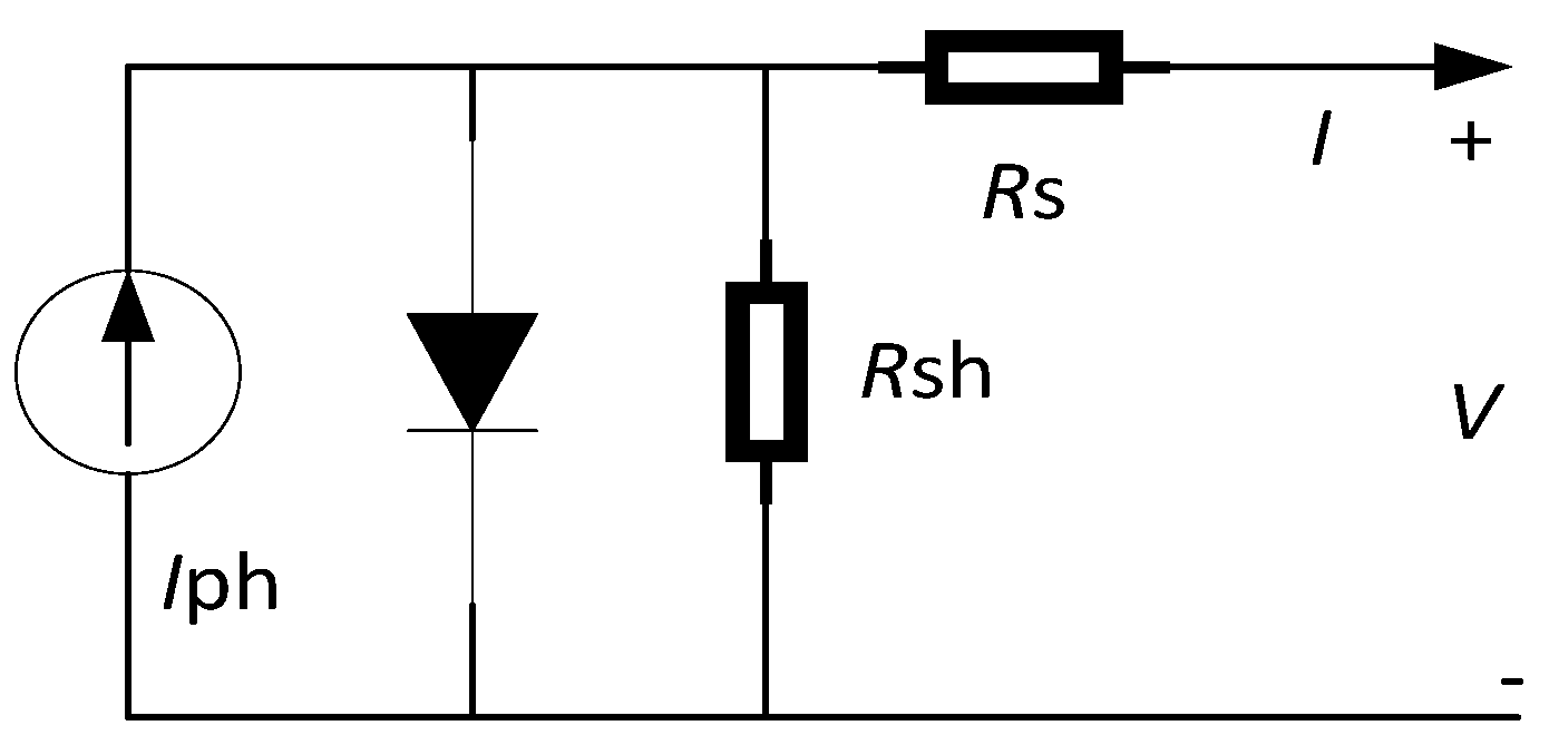
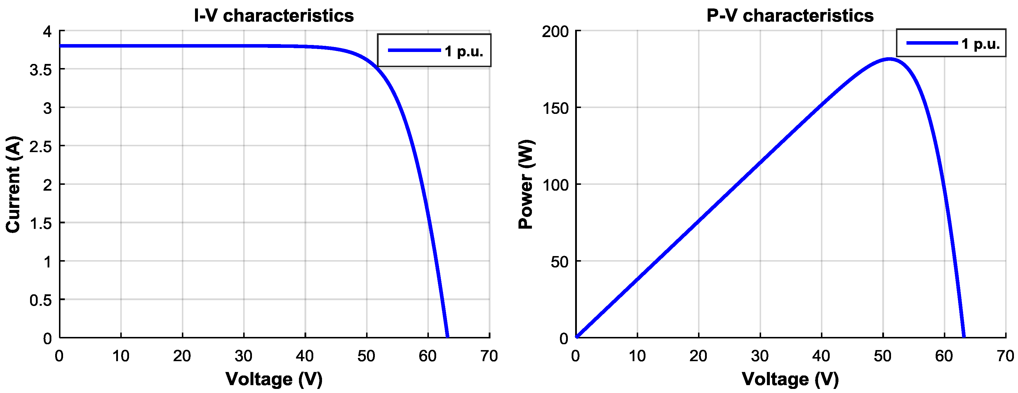
2.1. Model of Good Quality PV Cells

The single-diode model is widely adopted for modeling PV sources. Figure 1 shows the commonly used single-diode model of a PV module. The electrical model of the PV module is given by the authors of [23].

$$I=I_{ph}-I_s\left[e^{\left(\frac{q\left(V+I{R}_s\right)}{N_{s}KTA}\right)}-1\right]-\frac{\left(V+I{R}_s\right)}{R_{sh}}$$

(1)

where $q$ is the electron charge, $K$ is the Boltmann constant, $N_s$ is the number of series connected cells, $I_s$ is the diode saturation current (A), $A$ is the ideality factor, and $T$ is the module temperature (K). As shown in Figure 1, $I$ is the PV module output current (A), $I_{ph}$ is the photon current (A), $R_s$ is the series resistance (Ω), and $R_{sh}$ is the shunt resistance (Ω). The values of $q$ and $K$ are 1.6 × 10⁻¹⁹ C and 1.37 × 10⁻²³ J/K, respectively.

According to the authors of [10,24], for commercial solar cells, the shunt resistance, $R_{sh}$, is much greater than the forward resistance of the diode, and thus can be neglected for simplicity, and only the series resistance, $R_s$, will be considered. Therefore, Equation (1) is reduced to the following:

$$I=I_{ph}-I_s\left[e^{\left(\frac{q\left(V+I{R}_s\right)}{N_{s}KTA}\right)}-1\right]$$

(2)

In this research, the Solarex MSX60 PV module technical data sheet was used [23] and the aging factors used for simulation and illustration purposes were randomly generated. Each MSX60 PV module consists of 36 series connected polycrystalline cells, while the ideality, $A$, has been chosen as 1.2. The technical specifications of the Solarex MSX60 PV module are given in

Table 1. The key specifications of the Solarex MSX60 photovoltaic (PV) module [23].

At Temperature T = 25 °C
Open circuit voltage	$V_{OC}$	21.0 V
Short circuit current	$I_{SC}$	3.74 A
Voltage at max. power	$V_m$	17.1 V
Current at max. power	$I_m$	3.5 A
Maximum power	$P_m$	59.9 W

.

PV manufacturers typically provide the values of the open-circuit voltage ($V_{OC}$), short-circuit current ($I_{SC}$), and the maximum power point ($V_{MP}$, ${\mathrm{I}}_{\mathrm{MP}}$) at standard test conditions (STC).

• Short-circuit current is the maximum current that a PV cell can generate.
• Open-circuit voltage is the maximum voltage across a PV cell.
• Maximum power point (MPP) is the point on the I–V (voltage–current) characteristic curve where the product of voltage, $V_{MP}$, and current, ${\mathrm{I}}_{\mathrm{MP}}$, is the maximum [25].

In addition, a model proposed by the authors of [26] was used to study and evaluate the I–V and P–V characteristics of a PV array under non-uniform aging conditions.

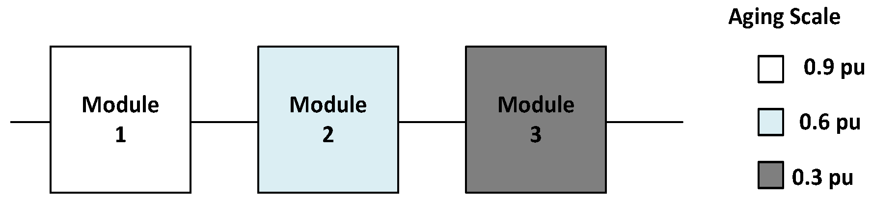
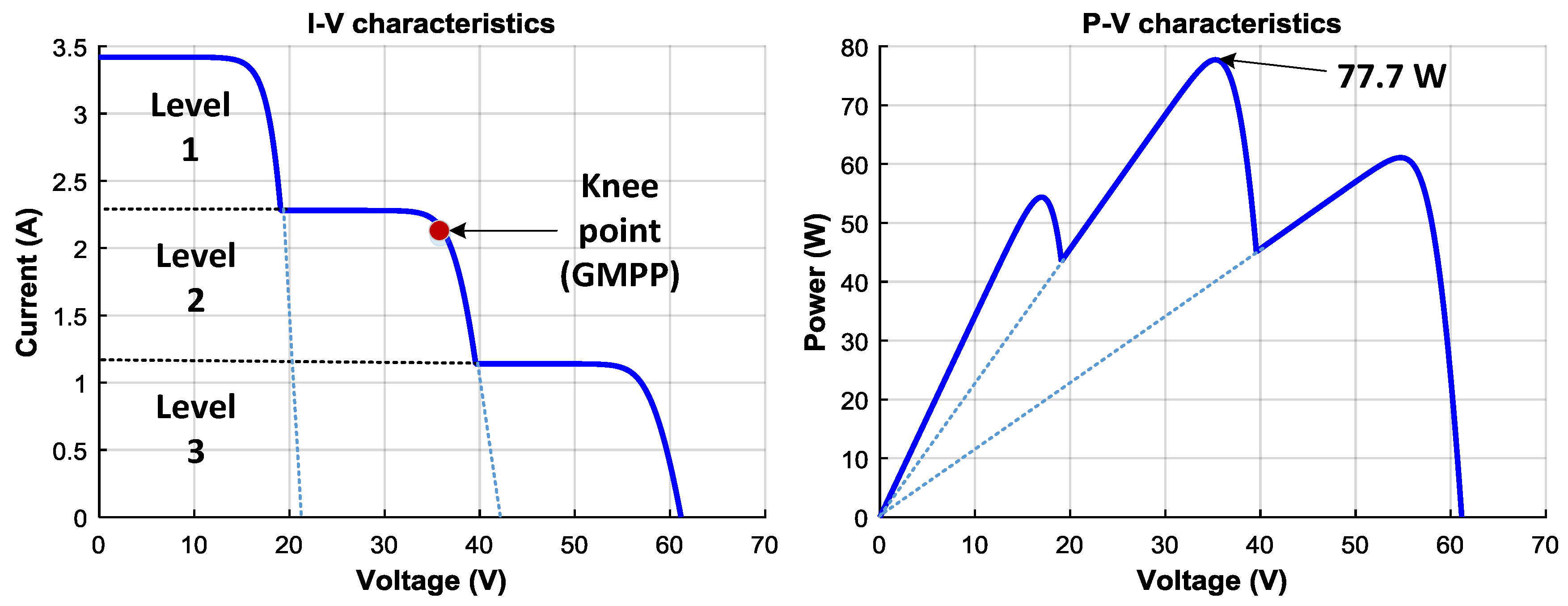
2.2. Mismatch Analysis Due to Non-Uniform Aging

According to the authors of [6], the short circuit current varies more than the open circuit voltage when a PV cell undergoes aging experiment, as a result of the $p$-$n$ junction characteristics of the cell. In this paper, we will use the short circuit current to evaluate the aging condition of the PV module, while keeping the open circuit voltage unchanged for different aging conditions. It is also assumed that all of the cell-units in the same PV module undergo uniform aging, so that the entire PV module can be characterised by a single maximum short-circuit of any of the cell-unit. In a PV array consisting of $m$ series-connected PV modules, the output current of the modules are equal to each other, and the output voltage is the sum of the total module voltages.

$$I_{total}=I_{module 1}=I_{module 2}=\cdots =I_{module m}$$

(3)

$$V_{total}=V_{module 1}+V_{module 2}+\cdots +V_{module m}={\displaystyle \sum }_{i=1}^m{V}_{module i}$$

(4)

Equations (3) and (4) are true when the modules are identical. Under good quality conditions, the three modules act identically and the voltages of the three modules are equal to a value of 63 V, as shown in Figure 2. Also, as the PV modules are identical, the same short-circuit current flows through the series-connected PV modules, which is equal to 3.74 A (see Figure 2).

However, during the non-uniform aging processes, there is a mismatch in the short-circuit current of the individual PV module. Each PV module is connected in parallel to a bypass diode, so as to avoid the occurrence of a hot spot. Figure 3 illustrates a series combination of three modules with different aging scales.

Because of the non-uniform aging condition, multiple steps and multiple peaks of the PV power output are observed in Figure 4. This categorises the operation of the PV array into three different operation levels, and each peak corresponds to a particular level. Level 1 corresponds to the stage where module 1 is active, while module 2 and module 3 are being bypassed by the diodes. At this level, the current is between 0 and 3.42 A, and the corresponding voltage is 0–21 V. Similarly, level 2 corresponds to the stage where module 1 and module 2 are active, while module 3 is being bypassed. The current for the un-bypassed series-connection is set by the current of the most aged PV module (in this case is the module 2). The current at level 2 is between 0 and 2.28 A, and the corresponding voltage is 0–42 V. Level 3 corresponds to the stage where all of the modules are active, that is, none of the modules are bypassed. Similarly, the current for the un-bypassed series connection is set by the current of the most aged PV module (in this case is the module 3). The current at level 3 is between 0 and 1.44, and the corresponding voltage is 0–61.2 V. Furthermore, there are multiple maximum power points showing from the knee points for the different levels in the I–V characteristic curve. These knee points correspond to certain currents and voltages that are used to obtain the maximum power points at different locations on the P–V curve. The knee point at level 1 operates at 16.98 V and 3.2 A, corresponding to 54.4 W, the knee point at level 2 operates at 34.58 V and 2.21 A corresponding to 77.7 W, while the knee point at level 3 operates at 54.69 V and 1.12 A, corresponding to 61.1 W, as illustrated in the P–V curve of Figure 4. The knee point at level 2 represents the global maximum power point (GMPP).

In the next section, the series-connected modules would form strings, which are connected in parallel to form an SP configuration with non-uniform aging conditions, so as to illustrate our proposed reconfiguration algorithm.

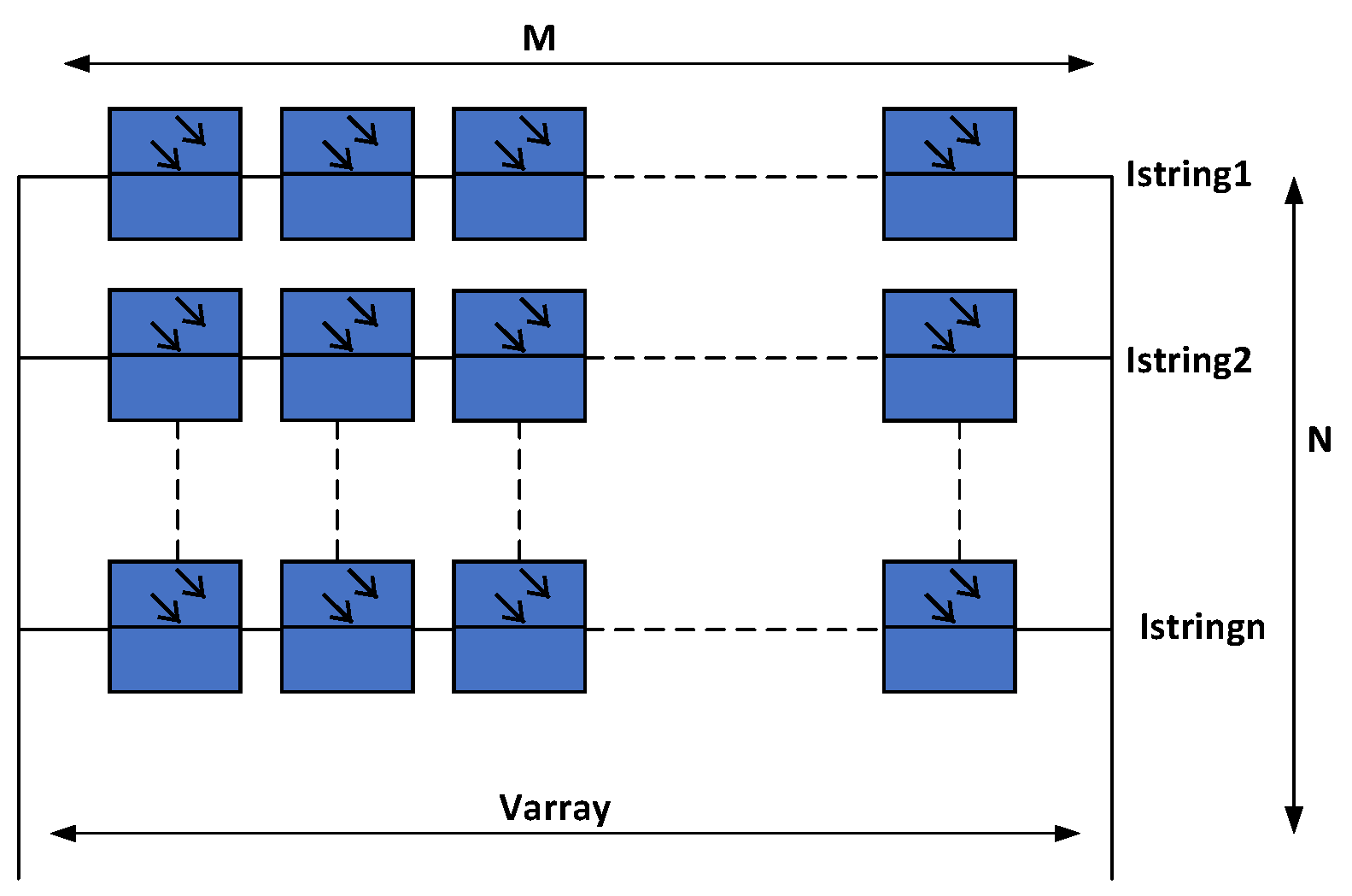
3. PV Array Reconfiguration Scheme

In an $\mathrm{N}\times \mathrm{M}$ PV array, $\mathrm{N}$ is the parallel-connected strings and $\mathrm{M}$ is the number of series-connected PV modules, as shown in Figure 5. It is worth noting that the voltage where the GMPP of a PV array is located in the P–V curve represents the number of active modules for a given string voltage. Therefore, the maximum power of the PV array is obtained by the product of the sum of all of the string currents and the string voltage of the active modules.

A PV array consisting of $16$ aged modules connected in a 4 × 4 SP configuration, shown in Figure 6, will be used to illustrate this concept.

In Figure 6, there are four parallel-connected strings (rows) and four series-connected modules (columns), while the per-unit values denote the non-uniform aging status in the PV array, which has a direct relationship to their individual short-circuit currents.

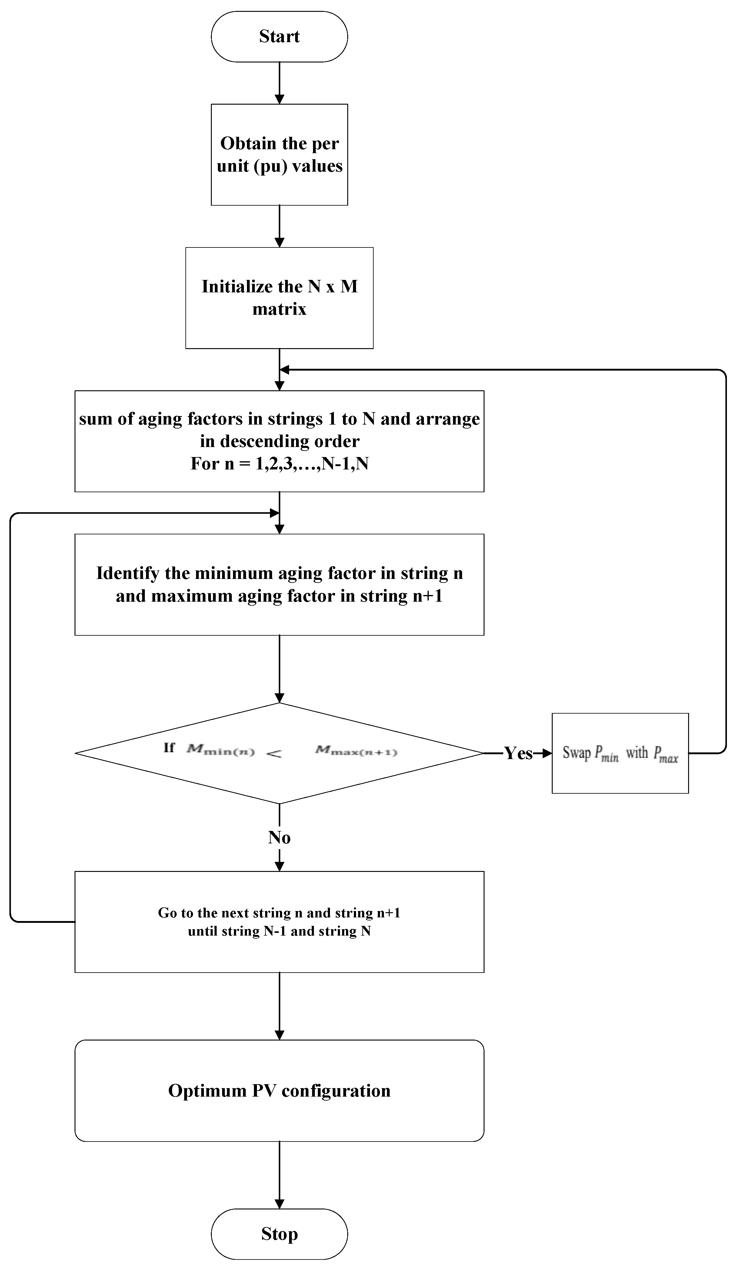
PV Reconfiguration Algorithm

Generally, the possible number of arrangements for an $\mathrm{N}\times \mathrm{M}$ PV array is $\left(\begin{array}{c}\mathrm{NM}\\ \mathrm{M}\end{array}\right)\left(\begin{array}{c}\mathrm{NM}-\mathrm{M}\\ \mathrm{M}\end{array}\right)\left(\begin{array}{c}\mathrm{NM}-2\mathrm{M}\\ \mathrm{M}\end{array}\right)\left(\begin{array}{c}\mathrm{NM}-3\mathrm{M}\\ \mathrm{M}\end{array}\right)\cdots \left(\begin{array}{c}2\mathrm{M}\\ \mathrm{M}\end{array}\right)\left(\begin{array}{c}\mathrm{M}\\ \mathrm{M}\end{array}\right)/\mathrm{N}!$. For the $4\times 4$ PV array, there will be 2,627,625 possible arrangements, and calculating the maximum power for all of the possible PV module arrangements for a large PV array (say larger values of $\mathrm{N}$ and $\mathrm{M}$) becomes very difficult. The proposed reconfiguration algorithm is based on an iterative and hierarchical sorting of PV modules, in order to achieve optimum configuration within several iterative steps. In the proposed algorithm, the aging scale (coefficient) shall be used as the varying parameter, as it is directly related to the short-circuit current of each individual PV module. The short-circuit current in a healthy module is set as 1 p.u. under the standard testing condition (STC), which represents 1000 W/m² irradiance and 25 °C module temperature. The digits in the array represent the different aging factors of the PV modules, which has a direct relationship to their individual short-circuit currents. Let’s consider a $4\times 4$ PV array configuration, shown in Figure 6.

The working parameter shall be the aging factor (AF), which has already been expressed as per unit (p.u.) value of the health status of the individual PV module.

The following parameters are defined in order to outline our proposed algorithm in six steps.

For n = 1, 2, 3, …, N − 1, N, where N is the number of strings in the PV array.

${{\displaystyle \sum }}^{}A{F}_{string n}$ = sum of aging factors in a series-connected string.

$M_{min\left(n\right)}$ = minimum aging factor in a series-connected modules for string n.

$P_{min}$ = position of PV module with minimum aging factor in a series-connected modules.

$M_{max\left(n+1\right)}$ = maximum aging factor in a series-connected modules for string n + 1.

$P_{max}$ = position of PV module with maximum aging factor in a series-connected modules.

Step 1: Obtain the summation of AFs for each string, as follows:

$${{\displaystyle \sum }}^{}A{F}_{string 1}=0.8+0.7+0.9+0.5=2.9$$

(5)

$${{\displaystyle \sum }}^{}A{F}_{string 2}=0.6+0.4+0.9+0.7=2.6$$

(6)

$${{\displaystyle \sum }}^{}A{F}_{string 3}=0.8+0.5+0.6+0.5=2.4$$

(7)

$${{\displaystyle \sum }}^{}A{F}_{string 4}=0.8+0.6+0.5+0.4=2.3$$

(8)

Step 2: Arrange the total string level AFs in a descending order, in the case study.

Step 3: Identify $M_{min\left(n\right)}$ and $M_{max\left(n+1\right)}$ for n = 1.

$$M_{min\left(1\right)}=0.5$$

(9)

$$M_{max\left(2\right)}=0.9$$

(10)

If $M_{min\left(1\right)}<M_{max\left(2\right)}$, then swap $P_{min}$ with $P_{max}$ and repeat Steps 1, 2, and 3.

Step 4: Repeat Steps 1, 2, and 3 until $M_{min\left(n\right)}\ge M_{max\left(n+1\right)}$.

Step 5: Identify $M_{min\left(n\right)}$ and $M_{max\left(n+1\right)}$ for n = 2, swap the corresponding $P_{min}$ with $P_{max}$, and repeat steps 1, 2, 3, and 4.

Step 6: Repeat step 5 until the end (N − 1).

From the last step, the array atthe right hand side (RHS) shows the optimum configuration. However, each of the configurations that arrived at each step were compared with the original arrangement, as shown in Figure 6. As illustrated for the $4\times 4$ PV array, only six iterative steps were needed to arrive at the optimum configuration for a non-uniform aging condition. Furthermore, a MATLAB program is written to execute for a large PV array, and the optimized form depicts the arrangements for the optimum power output. Therefore, for the instance of a $4\times 4$ PV array, the array “after” arrangement is the optimum configuration. Figure 7 shows the comparison between the PV array “before” and “after” arrangement.

The maximum power and voltage at MPP were tabulated in

Table 2. Electrical parameters obtained for different reconfigurations. MPP—maximum power point.

Steps	Maximum Power $\left({\mathit{P}}_{\mathit{m}}\right)$ (W)	Voltage at MPP $\left({\mathit{V}}_{\mathit{m}}\right)$ (V)	String Currents (A)
			1	2	3	4
1	468.6	71	1.863	1.492	1.757	1.482
2	515.6	70	2.587	1.793	1.490	1.488
3	530.7	70	2.818	1.779	1.490	1.488
4	535.3	70	2.818	1.859	1.488	1.475
5	558.6	70	2.818	2.206	1.475	1.475
6	573.7	69	2.867	2.260	1.790	1.428

for each configuration and the string currents in each case. Clearly, the total output power is increased by 22.4% between Step 1 and Step 6. Also, the voltage at MPP does not vary much compared to the output current. This algorithm maximizes the currents in each string by combining the PV modules with almost the same electrical characteristics, so as to reduce multiple peaks resulting from mismatch effects (non-uniform aging).

To execute the MATLAB program. the PV array shall be represented in matrix form, given by Equation (11).

$${\mathrm{N}\mathrm{by}\mathrm{M}}_{\mathrm{matrix}}=\left[\begin{array}{c}\begin{array}{ccc}0.8& 0.7& \begin{array}{cc}0.9& 0.5\end{array}\end{array}\\ \begin{array}{ccc}0.6& 0.4& \begin{array}{cc}0.9& 0.7\end{array}\end{array}\\ \begin{array}{c}\begin{array}{ccc}0.8& 0.5& \begin{array}{cc}0.6& 0.5\end{array}\end{array}\\ \begin{array}{ccc}0.8& 0.6& \begin{array}{cc}0.5& 0.4\end{array}\end{array}\end{array}\end{array}\right]$$

(11)

The flowchart of the reconfiguration algorithm for an $\mathrm{N}\times \mathrm{M}$ PV array is shown in Figure 5. The objective of this proposed algorithm is to swap the positions of the individual PV modules in each string, based on their aging factors, so as to reduce the effect of the mismatch losses amongst the PV modules in a particular string.

The developed algorithm requires only instantaneous short-circuit current information for data entry (represented as aging factors, as aging is directly related to the short-circuit current). Furthermore, the algorithm continues until all of the criteria are met, as illustrated in Figure 8, in order to obtain the optimum configuration.

4. Results and Discussions

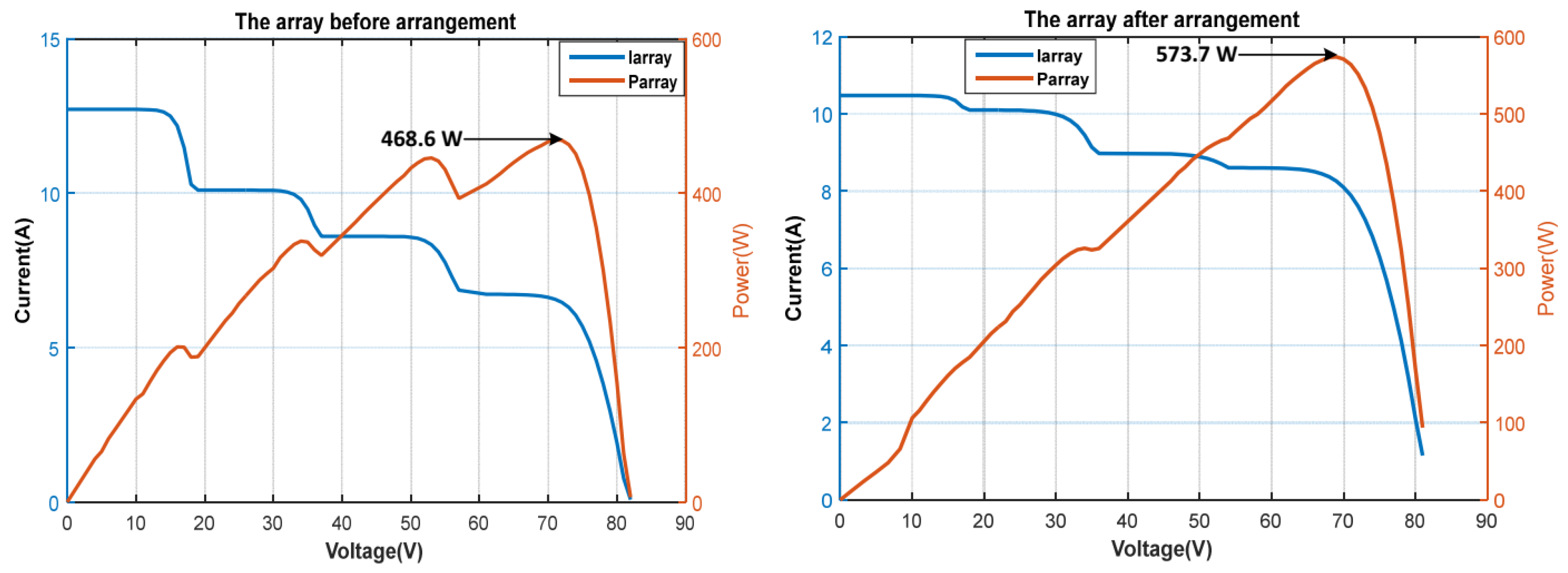
4.1. Simulation Results

In order to validate the proposed algorithm, PV arrays of different sizes will be considered, that is, 4 × 4, 10 × 10, and 100 × 10 PV arrays. The maximum output powers from the PV configuration before and after arrangement are obtained using a PV array model built in MATLAB.

A computer with Intel (R) Core (TM) i3-5005U CPU at 2.00 GHz, with 4 G RAM was used to perform the calculation and the corresponding computing time for a 4 × 4, 10 × 10, and 100 × 10 PV array tabulated.

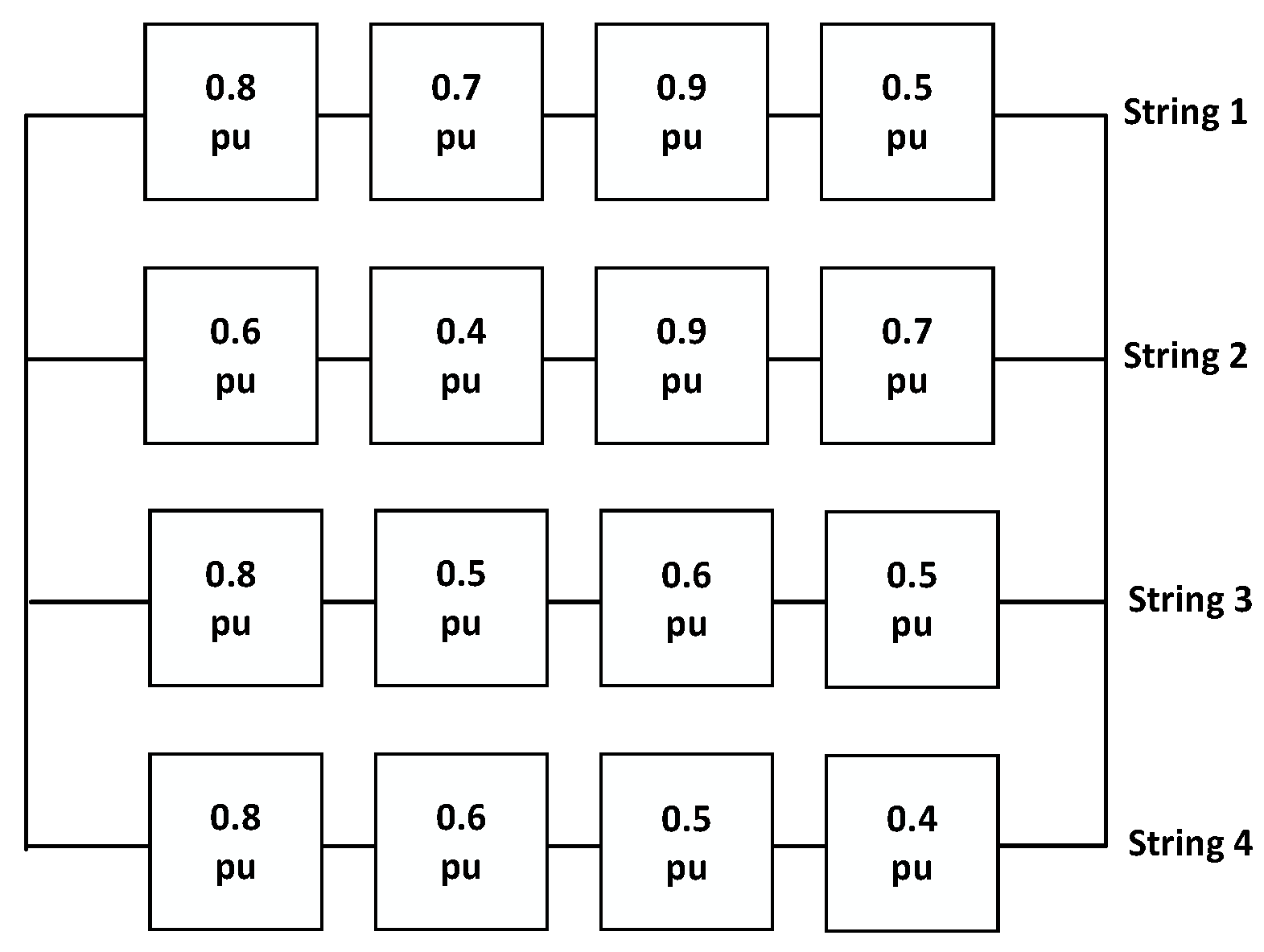
4.2. Case 1: 4 × 4 PV Array

Figure 6 will be used in this case to verify the results using MATLAB. The maximum short-circuit current in a healthy module is set as 1 p.u. under the standard testing condition (STC), which represents the 1000 W/m² irradiance and 25 °C module temperature.

In

Table 3. PV configuration before and after arrangement for Case 1.

Before Arrangement				After Arrangement
0.8 pu	0.7 pu	0.9 pu	0.5 pu	0.8 pu	0.8 pu	0.9 pu	0.9 pu
0.6 pu	0.4 pu	0.9 pu	0.7 pu	0.7 pu	0.8 pu	0.6 pu	0.7 pu
0.8 pu	0.5 pu	0.6 pu	0.5 pu	0.6 pu	0.6 pu	0.5 pu	0.5 pu
0.8 pu	0.6 pu	0.5 pu	0.4 pu	0.5 pu	0.4 pu	0.5 pu	0.4 pu

, the PV configuration after arrangement was obtained using the proposed algorithm. With the information of the PV array shown in Table 3, the $I-V$ and $P-V$ characteristic curves are plotted as shown in Figure 9. Figure 9 shows that the maximum output power before arrangement, which is 468.6 W, and the PV array output voltage and current for the GMPP are 71 V and 6.498 A, respectively. The maximum output power after arrangement is 573.7 W, and the PV array output voltage and current for the GMPP are 69 V and 8.255 A, respectively. Obviously, the total output power increases by 22.4% when the proposed algorithm is used. The computing time for the rearrangements of an aged 4 × 4 PV array takes 0.01 s to execute our proposed algorithm as shown in

Table 4. 4 × 4 PV array parameters (before and after arrangement).

Parameter	Before	After	Computing Time (s)	Power Improvement (Percentage)
$P_m$	$468.6\mathrm{W}$	$573.7 \mathrm{W}$	0.01	22.4%
$V_m$	$71 \mathrm{V}$	$69 \mathrm{V}$
$I_m$	$6.498 \mathrm{A}$	$8.255 \mathrm{A}$

.

4.3. Case 2: 10 × 10 PV Array

For a medium size $10\times 10$ PV array, there are 10 parallel-connected strings and 10 series-connected modules. Here, the aging factors, ranging from $0.4$ p.u. to $0.9$ p.u., were randomly generated in MATLAB (R2015a) to form a $10\times 10$ matrix, replicating a non-uniform aging PV array before arrangement, as shown in

Table 5. PV configuration before and after arrangement for Case 2.

Before Arrangement
$0.4$ pu	$0.6$ pu	$0.4$ pu	$0.6$ pu	$0.9$ pu	$0.6$ pu	$0.8$ pu	$0.5$ pu	$0.7$ pu	$0.9$ pu
$0.8$ pu	$0.4$ pu	$0.9$ pu	$0.9$ pu	$0.7$ pu	$0.4$ pu	$0.6$ pu	$0.6$ pu	$0.5$ pu	$0.8$ pu
$0.5$ pu	$0.5$ pu	$0.4$ pu	$0.5$ pu	$0.6$ pu	$0.9$ pu	$0.5$ pu	$0.8$ pu	$0.8$ pu	$0.6$ pu
$0.7$ pu	$0.9$ pu	$0.8$ pu	$0.5$ pu	$0.7$ pu	$0.9$ pu	$0.6$ pu	$0.4$ pu	$0.5$ pu	$0.6$ pu
$0.4$ pu	$0.4$ pu	$0.8$ pu	$0.4$ pu	$0.6$ pu	$0.6$ pu	$0.4$ pu	$0.4$ pu	$0.8$ pu	$0.6$ pu
$0.7$ pu	$0.8$ pu	$0.9$ pu	$0.4$ pu	$0.4$ pu	$0.6$ pu	$0.4$ pu	$0.5$ pu	$0.5$ pu	$0.5$ pu
$0.5$ pu	$0.7$ pu	$0.4$ pu	$0.9$ pu	$0.5$ pu	$0.6$ pu	$0.9$ pu	$0.7$ pu	$0.6$ pu	$0.7$ pu
$0.7$ pu	$0.9$ pu	$0.6$ pu	$0.7$ pu	$0.4$ pu	$0.9$ pu	$0.9$ pu	$0.8$ pu	$0.7$ pu	$0.7$ pu
$0.8$ pu	$0.4$ pu	$0.5$ pu	$0.7$ pu	$0.5$ pu	$0.6$ pu	$0.7$ pu	$0.7$ pu	$0.8$ pu	$0.8$ pu
$0.8$ pu	$0.6$ pu	$0.8$ pu	$0.4$ pu	$0.5$ pu	$0.4$ pu	$0.4$ pu	$0.6$ pu	$0.4$ pu	$0.8$ pu
After Arrangement
$0.9$ pu	$0.9$ pu	$0.9$ pu	$0.9$ pu	$0.9$ pu	$0.9$ pu	$0.9$ pu	$0.9$ pu	$0.9$ pu	$0.9$ pu
$0.9$ pu	$0.8$ pu	$0.8$ pu	$0.8$ pu	$0.9$ pu	$0.9$ pu	$0.8$ pu	$0.8$ pu	$0.8$ pu	$0.8$ pu
$0.8$ pu	$0.8$ pu	$0.8$ pu	$0.8$ pu	$0.8$ pu	$0.8$ pu	$0.8$ pu	$0.8$ pu	$0.7$ pu	$0.8$ pu
$0.7$ pu	$0.7$ pu	$0.7$ pu	$0.7$ pu	$0.7$ pu	$0.7$ pu	$0.7$ pu	$0.7$ pu	$0.7$ pu	$0.7$ pu
$0.7$ pu	$0.6$ pu	$0.6$ pu	$0.6$ pu	$0.7$ pu	$0.6$ pu	$0.6$ pu	$0.7$ pu	$0.7$ pu	$0.6$ pu
$0.6$ pu	$0.6$ pu	$0.6$ pu	$0.6$ pu	$0.6$ pu	$0.6$ pu	$0.6$ pu	$0.6$ pu	$0.6$ pu	$0.6$ pu
$0.5$ pu	$0.5$ pu	$0.5$ pu	$0.6$ pu	$0.5$ pu	$0.6$ pu	$0.5$ pu	$0.5$ pu	$0.5$ pu	$0.6$ pu
$0.5$ pu	$0.5$ pu	$0.5$ pu	$0.5$ pu	$0.5$ pu	$0.5$ pu	$0.4$ pu	$0.5$ pu	$0.5$ pu	$0.5$ pu
$0.4$ pu	$0.4$ pu	$0.4$ pu	$0.4$ pu	$0.4$ pu	$0.4$ pu	$0.4$ pu	$0.4$ pu	$0.4$ pu	$0.4$ pu
$0.4$ pu	$0.4$ pu	$0.4$ pu	$0.4$ pu	$0.4$ pu	$0.4$ pu	$0.4$ pu	$0.4$ pu	$0.4$ pu	$0.4$ pu

, as well as the optimum PV configuration (after arrangement) for this case. These two PV configurations were simulated and the result shows that the proposed algorithm gives an optimum configuration. Figure 10 shows that the maximum output power before arrangement is $2754 \mathrm{W}$, and the PV array output voltage and current for the GMPP are $164 \mathrm{V}$ and $16.95 \mathrm{A}$, respectively. The maximum output power after arrangement is $3920 \mathrm{W}$, and the PV array output voltage and current for the GMPP are $171 \mathrm{V}$ and $21.13 \mathrm{A}$, respectively. The computing time for the rearrangements of an aged $10\times 10$ PV array takes $0.035 \mathrm{s}$ to execute in our proposed algorithm as shown in

Table 6. 10 × 10 PV array parameters (before and after arrangement).

Parameter	Before	After	Computing Time (s)	Power Improvement (Percentage)
$P_m$	$2754\mathrm{W}$	$3624\mathrm{W}$	0.035	31.6%
$V_m$	$164\mathrm{V}$	$171\mathrm{V}$
$I_m$	$16.95\mathrm{A}$	$21.13\mathrm{A}$

.

4.4. Case 3: 100 × 10 PV Array

For a large PV array, say a $100\times 10$ array with 100 parallel-connected strings and 10 series-connected modules. The non-uniform aging factors were randomly generated, as in Case 2. It was observed that the power improved by 36.7% when the proposed algorithm was applied, and the average computing time was 2.746 s, as shown in

Table 7. 100 × 10 PV array parameters (before and after arrangement).

Parameter	Before	After	Computing Time (s)	Power Improvement (Percentage)
$P_m$	$27.69\mathrm{kW}$	$37.85\mathrm{kW}$	2.746	36.7%
$V_m$	$165\mathrm{V}$	$168\mathrm{V}$
$I_m$	$167\mathrm{A}$	$223\mathrm{A}$

.

4.5. Discussions

From the results obtained for the three cases, it is observed that the proposed algorithm can be applicable to different sizes of PV arrays, and an improved maximum power has been achieved for the three cases. In addition, the proposed algorithm minimizes the effect of the bypass diodes by swapping the positions of the individual PV modules in each string based on their aging factors, so as to reduce the effect of mismatch losses amongst PV modules in a particular string, but the voltage limitation was not considered in this work, as discussed by the authors of [22]. This algorithm involves a hierarchical and iterative sorting of the PV modules. The P − V curves (see Figure 9, Figure 10 and Figure 11) for the three cases show that the effect of mismatch amongst the PV modules has been reduced after the rearrangement. Moreover, this proposed algorithm does not need to access all of the possible configurations for a particular PV array (huge number), which makes it relatively faster. For instance, in Case 1, only six steps were needed for the algorithm to arrive at the optimum arrangement (configuration) without having to go through all 2,627,625 possible arrangements. The computing time for the three cases was recorded in Table 4, Table 5, Table 6 and Table 7. In other words, the optimal configuration with the proposed algorithm can be found in a short time and can in turn be applied for implementation in real time. Interestingly, the affected PV modules to be swapped are the only ones involved in the transition, while the rest remain in their original position, therefore reducing the number of relays to be used for switching purposes, which in turn saves on cost and time compared with that proposed in refs. [6,22].

5. Conclusions

In this work, we studied and analysed the non-uniform aging processes in the PV arrays, and we found that the locations of aged PV modules in the PV arrays influence the power generation of the solar PV arrays. In order to alleviate the negative influence of non-uniformly aging PV arrays, we propose a novel PV array reconfiguration algorithm to maximize the power generation from non-uniformly aged PV arrays, without replacing the aged PV modules with new ones. In this algorithm, the PV modules are sorted iteratively in a hierarchy pattern so as to reduce the effect of mismatch due to non-uniform aging amongst PV modules, and the maximum power output has improved by 22.4%, 31.6%, and 36.7% for the 4 × 4, 10 × 10, and 100 × 10 arrays, respectively.

Compared to the existing online PV array reconfiguration methods, the proposed PV module rearrangement approach requires fewer relays but effectively boost the PV systems’ maximum power output. The proposed algorithm is also easily implementable, as it only requires swapping locations of the PV modules.

References

1. Sanseverino, E.R.; Ngoc, T.N.; Cardinale, M.; Vigni, V.L.; Musso, D.; Romano, P.; Viola, F. Dynamic programming and munkres algorithm for optimal pv arrays reconfiguration. Sol. Energy 2015, 122, 347–358. [Google Scholar] [CrossRef]
2. International Renewable Energy Agency (IRENA), Renewable Power Generation Costs in 2017. Available online: https://www.irena.org//media/Files/IRENA/Agency/Publication/2018/Jan/IRENA_2017_Power_Costs_2018.pdf (accessed on 12 September 2018).
3. Banavar, M.; Braun, H.; Buddha, S.T.; Krishnan, V.; Spanias, A.; Takada, S.; Takehara, T.; Tepedelenlioglu, C.; Yeider, T. Signal processing for solar array monitoring, fault detection, and optimization. Ynth. Lect. Power Electron. 2012, 7, 1–95. [Google Scholar] [CrossRef]
4. Photovoltaics Report, Fraunhofer ISE and Werner Warmuth, PSE Conferences & Consulting GmbH, 27 August 2018. Available online: hhtps://www.ise.fraunhofer.de (accessed on 12 September 2018).
5. Goodrich, A.; James, T.; Woodhouse, M. Residential, commercial and utility-scale PV system prices in the US: Current drivers and cost-reduction opportunities. Natl. Renew. Energy Lab. 2012. [Google Scholar] [CrossRef]
6. Hu, Y.; Zhang, J.; Wu, J.; Cao, W.; Tian, G.Y.; Kirtley, J.L. Efficiency of non-uniformly aged PV array. IEEE Trans. Power Electron. 2017, 32, 1124–1137. [Google Scholar] [CrossRef]
7. Ndiaye, A.; Kébé, C.M.; Ndiaye, P.A.; Charki, A.; Kobi, A.; Sambou, V. A novel method for investigating photovoltaic module degradation. Energy Procedia 2013, 36, 1222–1231. [Google Scholar] [CrossRef]
8. Mekhilefa, S.; Saidurb, R.; Kamalisarvestanib, M. Effect of dust, humidity and air velocity on efficiency of photovoltaic cells. Renew. Sustain. Energy Rev. 2012, 16, 2920–2925. [Google Scholar] [CrossRef]
9. Cristaldi, L.; Faifer, M.; Rossi, M.; Toscani, S.; Catelani, M.; Ciani, L.; Lazzaroni, M. Simplified method for evaluating the effects of dust and aging on photovoltaic panels. Measurement 2014, 54, 207–214. [Google Scholar] [CrossRef]
10. Femia, N.; Petrone, G.; Spagnuolo, G.; Vitelli, M. Power Electronics and Control Techniques for Maximum Energy Harvesting in Photovoltaic Systems; CRC Press: Boca Raton, FL, USA, 2012. [Google Scholar]
11. Balato, M.; Costanzo, L.; Vitelli, M. Reconfiguration of PV modules: A tool to get the best compromise between maximization of the extracted power and minimization of localized heating phenomena. Sol. Energy 2016, 138, 105–118. [Google Scholar] [CrossRef]
12. Kaplanis, S.; Kaplani, E. Energy performance and degradation over 20 years performance of BP c-Si PV modules. Simul. Model. Pract. Theory 2011, 19, 1201–1211. [Google Scholar] [CrossRef]
13. Shirzadi, S.; Hizam, H.; Wahab, N.I.A. Mismatch losses minimization in photovoltaic arrays by arranging modules applying a genetic algorithm. Sol. Energy 2014, 108, 467–478. [Google Scholar] [CrossRef]
14. Manganiello, P.; Balato, M.; Vitelli, M. A survey on mismatching and aging of PV Modules: The closed loop. IEEE Trans. Ind. Electron. 2015, 62, 7276–7286. [Google Scholar] [CrossRef]
15. La Manna, D.; Vigni, V.L.; Sanseverino, E.R.; Di Dio, V.; Romano, P. Reconfigurable electrical interconnection strategies for photovoltaic arrays: A review. Renew. Sustain. Energy Rev. 2014, 33, 412–426. [Google Scholar] [CrossRef]
16. Malathy, S.; Ramaprabha, R. Comprehensive analysis on the role of array size and configuration on energy yield of photovoltaic systems under shaded conditions. Renew. Sustain. Energy Rev. 2015, 49, 672–679. [Google Scholar] [CrossRef]
17. Camarillo-Peñaranda, J.R.; Ramírez-Quiroz, F.A.; González-Montoya, D.; Bolaños-Martínez, F.; Ramos-Paja, C.A. Reconfiguration of photovoltaic arrays based on genetic algorithm. Rev. Fac. Ing. Univ. Antioq. 2015, 95–107. [Google Scholar] [CrossRef]
18. Auttawaitkul, Y.; Pungsiri, B.; Chammongthai, K.; Okuda, M. A method of appropriate electrical array reconfiguration management for photovoltaic powered car. In Proceedings of the 1998 IEEE Asia-Pacific Conference on Circuits and Systems. Microelectronics and Integrating Systems (Cat. No.98EX242), Chiangmai, Thailand, 24–27 November 1998; pp. 201–204. [Google Scholar]
19. Chang, C. Solar Cell Array Having Lattice or Matrix Structure and Method of Arranging Solar Cells and Panels. U.S. Patent 6635817 B2, 21 October 2003. [Google Scholar]
20. Sherif, R.A.; Boutros, K.S. Solar Module Array with Reconfigurable Tile. U.S. Patent 6350944 B1, 26 February 2002. [Google Scholar]
21. Nguyen, D.; Lehman, B. An adaptive solar photovoltaic array using model-based reconfiguration algorithm. IEEE Trans. Ind. Electron. 2008, 55, 2644–2654. [Google Scholar] [CrossRef]
22. Hu, Y.; Zhang, J.; Li, P.; Yu, D.; Jiang, L. Non-Uniform Aged Modules Reconfiguration for Large-Scale PV Array. IEEE Trans. Device Mater. Reliab. 2017, 17, 560–569. [Google Scholar] [CrossRef]
23. Walker, G. Evaluating MPPT converter topologies using a Matlab PV Model. J. Electr. Electron. Eng. Aust. 2001, 21, 49–56. [Google Scholar]
24. Castaner, L.; Silvestre, S. Modelling Photovoltaic Systems Using PSpice; John Wiley and Sons Ltd.: Hoboken, NJ, USA, 2002. [Google Scholar]
25. Mahmoud, Y.A.; Xiao, W.; Zeineldin, H.H. A parameterization approach for enhancing PV model accuracy. IEEE Trans. Ind. Electron. 2013, 60, 5708–5716. [Google Scholar] [CrossRef]
26. Braun, H.; Buddha, S.T.; Krishnan, V.; Tepedelenlioglu, C.; Spanias, A.; Banavar, M.; Srinivasan, D. Topology reconfiguration for optimization of photovoltaic array output. Sustain. Energy Grids Netw. 2016, 6, 58–69. [Google Scholar] [CrossRef] [Green Version]
Figure 1. Single diode model.
Energies 11 02743 g001
Figure 2. I–V (voltage–current) and P–V (power–voltage) characteristics for series connection of good quality modules under standard test conditions.
Energies 11 02743 g002
Figure 3. Series-connection of photovoltaic (PV) modules.
Energies 11 02743 g003
Figure 4. I–V and P–V characteristics for series connection under non-uniform aging condition.
Energies 11 02743 g004
Figure 5. An N × M (parallel-connected strings × number of series-connected PV modules) (PV array (series parallel (SP) configuration).
Energies 11 02743 g005
Figure 6. A 4 × 4 SP configuration with non-uniform aging.
Energies 11 02743 g006
Figure 7. PV Array “before” and “after” rearrangement.
Energies 11 02743 g007
Figure 8. Flow chart of reconfiguration strategy.
Energies 11 02743 g008
Figure 9. The array output (before and after arrangement) for case 1.
Energies 11 02743 g009
Figure 10. The array output (before and after arrangement) for Case 2.
Energies 11 02743 g010
Figure 11. The array output (before and after arrangement) for Case 3.
Energies 11 02743 g011