A Sketch of Bolivia’s Potential Low-Carbon Power System Configurations. The Case of Applying Carbon Taxation and Lowering Financing Costs

Abstract

This paper considers hypothetical options for the transformation of the Bolivian power generation system to one that emits less carbon dioxide. Specifically, it evaluates the influence of the weighted average cost of capital (WACC) on marginal abatement cost curves (MACC) when applying carbon taxation to the power sector. The study is illustrated with a bottom-up least-cost optimization model. Projections of key parameters influence the shape of MACCs and the underlying technology configurations. These are reported. Results from our study (and the set of assumptions on which they are based) are country-specific. Nonetheless, the methodology can be replicated to other case studies to provide insights into the role carbon taxes and lowering finance costs might play in reducing emissions.

1. Introduction

Scientific evidence of the human influence on the climate system suggests that the increased concentration of anthropogenic greenhouse gases in the atmosphere is the dominant cause to the observed climate change [1]. In this regard, investments worldwide in the order of trillions of US$ in low-carbon energy generation and energy efficiency are needed to reach the 2 °C climate stabilization goal of the UNFCCC (United Nations Framework Convention of Climate Change, Paris Agreement 2015) [2]. Worldwide, the number of carbon pricing initiatives implemented or scheduled for implementation has reached 51 in 2018, and 88 parties have submitted emission pledges with proposals for carbon pricing mechanisms at the Paris Conference of Parties in 2015 [3]. Together the current carbon pricing schemes cover about half their emissions, which translates to about 13 percent of annual greenhouse gases (GHG) emissions worldwide.

Price-based or market-based policy instruments can take the form either of carbon taxes, energy taxes or emissions caps. Carbon taxes are aimed at reducing emissions according to the ‘polluter pays principle’. Current carbon prices vary significantly, from less than US$1 per tCO_2,e to up to US$131 per tCO_2,e [4]. An energy tax is levied on energy production from fossil fuels and aims at achieving a more efficient use of energy. However, if the goal is to reduce carbon emissions, a carbon tax is more cost-effective than an energy tax because it directly targets carbon content. In our study, we focus on the analysis of a carbon tax applied to the power generation system.

Globally, around 85 percent of emissions are priced at less than US$10 per tCO_2,e., which is lower than the range of 40 to 80 US$ per tCO_2,e identified by climate models to achieve the temperature stabilization goal [3]. A direct tax on greenhouse gas emissions is, in principle, an easy way to collect fiscal revenues and can contribute to financial incentives for renewable energy projects [4].

Technology development is a crucial factor towards a full-scale transition to renewable energy. Over the past decades, renewable energy technology costs have reduced remarkably. For example, the global average levelized cost of electricity (LCOE) of utility-scale solar photovoltaics declined by around 58% between 2010 and 2015 and still has 57% reduction potential in the next 10 years [5]. However, still one of the main challenges is to create attractive financial conditions for renewable energy technology (RET) investments [6].

Since the Kyoto Protocol, legal commitments to reduce GHG have driven analysis to find cost-efficient policies to meet these obligations. Marginal abatement cost curves (MACC) have been widely used to illustrate and compare the abatement costs of emissions of a set of mitigation alternatives. A detailed description of the use of the MACCs is provided in the articles of Ellerman et al., Kesicki et al. and Criqui et al. [7,8,9]. MACCs are unique for every country and delineated by several factor such as specific structure of the energy supply, energy prices and the potential to access to RET [8]. A recent review article reports 86 articles published in about a decade with applied examples of MACCs in climate policy research [10]. Examples of MAC analysis in long-term power generation planning and carbon taxation include studies by Van den Bergh et al. and Gollop et al. [11,12].

As part of the global community who have ratified the Paris Agreement “Bolivia will make an ambitious contribution in the context of national efforts” to mitigate GHG emissions [13]. This short analysis derives insights on the role of hypothetically increasing GHG taxes (or equivalent GHG mitigation subsidies) and reducing the WACC on emission reductions and cost-optimal technology configurations. For this purpose, a detailed bottom-up least-cost optimization model of the power sector of Bolivia is presented and average MACCs are illustrated. The article further illustrates how variations in projections of key parameters influence the MACCs. To date, no open-source computational energy model exists in literature that describe in detail the responses of emission-control policies in the Bolivian power sector. The peculiarities of this country make it of great interest for this analysis.

The article proceeds as follows: Section 2 summarizes relevant national information. Section 3 describes the key assumptions in the energy model. Section 4 describes results for the WACC, carbon tax and parameter sensitivity scenarios. Finally, Section 5 and Section 6 discuss specific conclusions of our analysis.

2. Short Background of Power Generation and Climate Policy in Bolivia

Due to its large reserves of natural gas, the Bolivian power system is dominated by gas combustion. In 2017, the 2.3 GW installed capacity (Considering grid: 2.1 GW and off-grid: 0.2 GW systems) 73% was gas fired, 26% was hydropower, and the final 1% was produced by biomass, solar and wind power [14]. Despite its large hydropower potential, to date, Bolivia has exploited less than 1% of its potential capacity [15]. Similarly, other renewable sources are still untapped.

Electricity prices remain low compared with other countries in South America. In part, this is due to high energy subsidies, that in turn represent a fiscal burden for the country (6.77% of GDP post-tax in 2015) [16]. In terms of electrification, 88% of Bolivians have access to the grid, with higher rates in urban areas (around 98%), and lower rates in rural areas (around 66%) [17]. A full electrification target was proposed to 2025 following to the Bolivia’s “Electricity for Life with Dignity” program [18].

Bolivia is a developing country with several challenges regarding, among others, poverty eradication, public health, food security and energy access. In spite of these challenges, Bolivia participated in international climate change negotiations and developed a National Mechanism for Adaptation to Climate Change. In October 2015, Bolivia submitted for the first time its Intended Nationally Determined Contribution (INDC) to the United Nations. The INDCs describe the commitment of the country to increase the efficiency of gas fired generation by upgrading to gas combined cycle and to increase the renewable energy capacity through large investments on hydropower, to not only meet local demands but to also export surplus by 2030 [13].

To date, no carbon pricing instruments nor emission reduction targets have been discussed in the climate action plans for Bolivia. In contrast, more than two thirds of Latin American and Caribbean nations’ climate action plans refer to the use of carbon pricing mechanisms to achieve the key objective of the Paris Agreement [19]. Brazil has a federal fuel tax (Contribution of Intervention in the Economic Domain, CIDE tax) levied in specific fuels and committed to reduce 6% of its GHG emissions in 2025 and 16% in 2030 below 1990 levels. In 2014, Mexico imposed a tax in several fossil fuels averaging 3US$/tonne CO_2,e and committed to reduce by 22% its GHG emissions in 2030. In 2017, Chile’s carbon tax came into effect and targets thermal power plants at 5 US$/tonne CO_2,e and committed on its INDC to cutting GHG emissions to 20% below 2007 levels by 2020. As it does not yet exist in the literature, research is required to provide related insights for policy design specifically in Bolivia.

3. Methodology

This section and the following paragraphs describe the energy system model developed for Bolivia. It includes an outline of parameter sensitivity analysis, carbon tax scenarios, description of the metrics and the software used for the study.

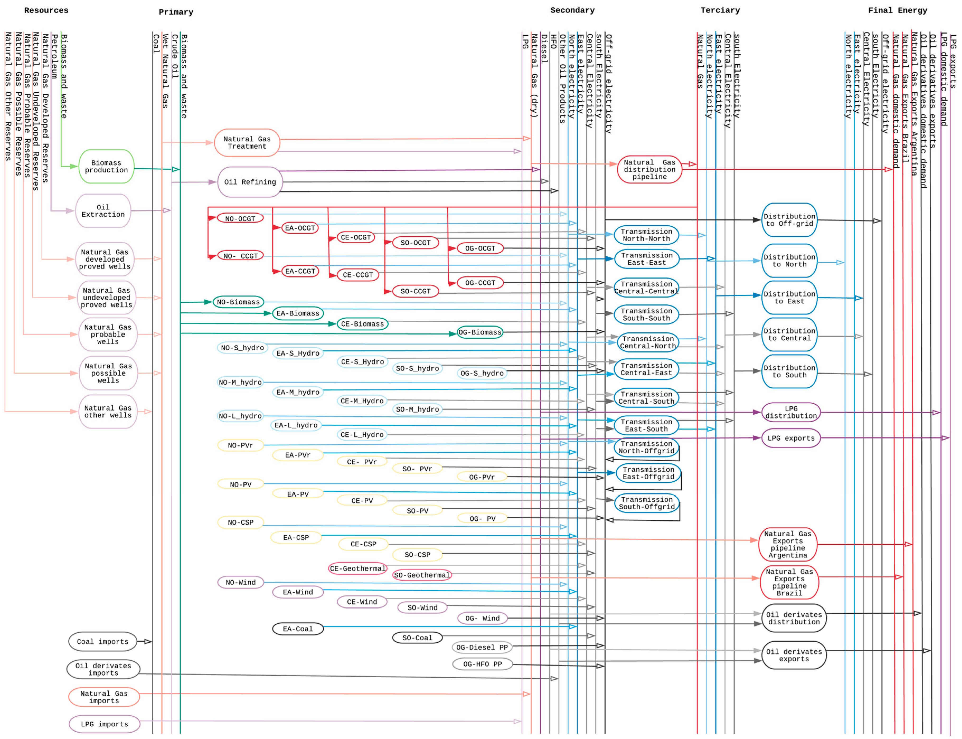
3.1. Energy System Model

3.1.1. Key Assumptions and Reference Energy Scenario

The model was designed assuming price-inelastic demand, free competition with no market imperfections, and predetermined projections for energy demand, fuel prices, renewable technology costs, resources availability, and environmental policy. The decision to invest and operate generation technologies is driven by the objective to minimize the total net present value of the system.

The model is deterministic. Uncertainty surrounding demand, fuel prices and technology costs are not modeled.

The cost of individual technologies chosen is a function of fuel, investment, operating, and maintenance costs. The configuration of technologies is driven by thermodynamic, emissions and other constraints such as meeting energy demands. A single discount rate was used for all technologies and kept constant for the entire model horizon. In the context of the model used, the discount rate is equal to the weighted average cost of capital (WACC). While it is common practice to use the WACC as the discount rate in capital budgeting, the authors use the terms discount rate, WACC and financing cost interchangeably (as they stand for the same concept) along the article. Technology-specific investor hurdle rates were not analyzed. The transmission infrastructure representation was simplified with the use of aggregated technologies with average efficiency and no contingency or reliability analysis was developed. The assumptions chosen are a deliberate simplification as the objective of the paper is to derive tractable insight related to the dynamics of hypothetical system configurations—rather than attempt to predict actual outcomes (or hedge for potential outcomes in the face of uncertainty). We would argue that the latter is important, but a subsequent step.

Electricity demand projections were used from Peña et al. [20] and sub-region split was calculated using a scenario construction methodology from CNDC [21]. Electricity demands projections for off-grid power systems and electricity demands for planned energy-intensive projects were included in each sub-region according data from the Ministry of Energy [17]. To account in the energy balance for other fuel demands relevant to electricity generation, projections for natural gas, LPG, and diesel demands were included from Peña et al. [20]. The reference scenario assumes a WACC of 12% constant for the entire modelling period and no carbon tax is considered.

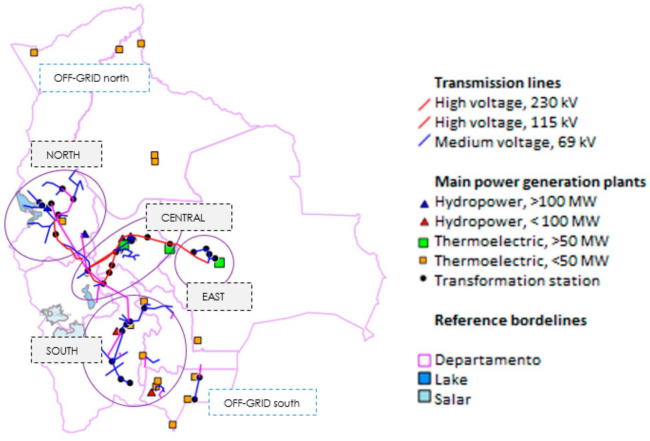
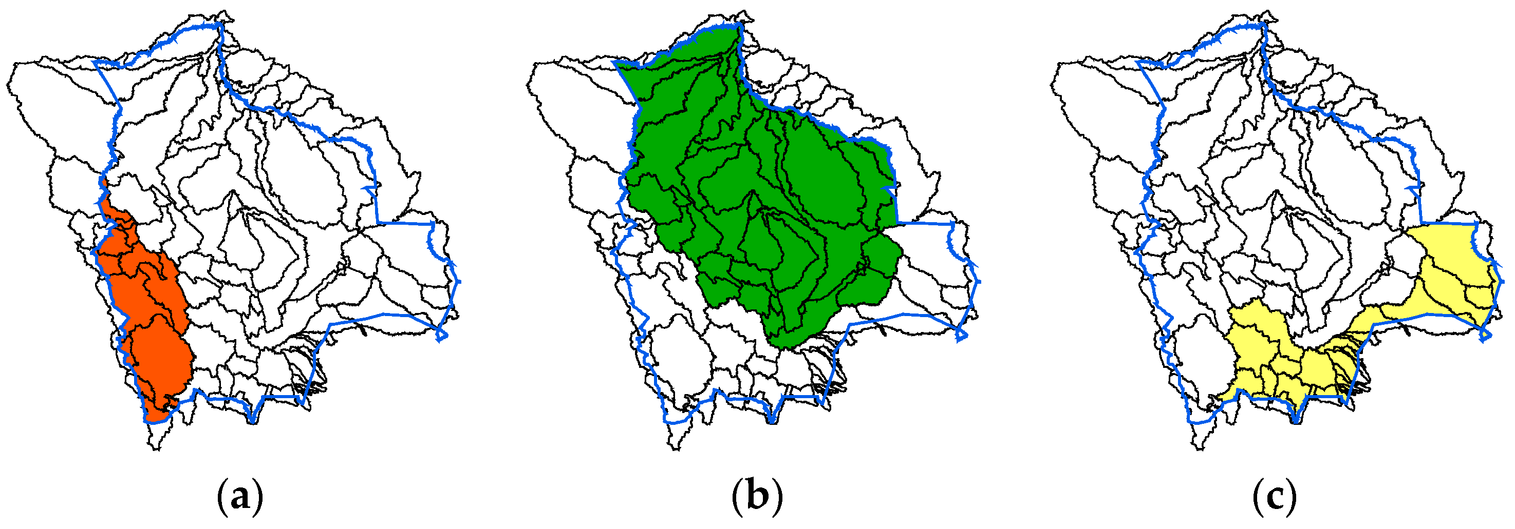
3.1.2. Model Spatial and Temporal Resolution

The model horizon 2013–2040 was selected to consider investments and policy effects taking place after the replacement of the existing infrastructure. A sub-regional representation (five sub-regions, as seen in Figure 1) was used to capture differences in demand, installed capacity, energy resources and fuel access. No dynamic trade interactions with other countries were included. Currently, the country is self-sufficient in electricity and despite several planned investments to export electricity, such projects were not included in this study due to their large size (larger than the current installed capacity of the entire country) and the uncertainty of their implementation. To capture temporal (particularly monthly) variations in resource availability and energy demands, each year was divided into time segments (or time-slices). A total of 48 time-slices (consisting of a simplified breakdown of 12 months, 1 day type and 4 equal day parts) per year were modelled. Hourly data of final electricity demand was used to calculate the average demand in each time-slice. This simplified time-sliced demand profile was assumed to remain constant for all years modelled. Note that increasing time-slice resolution comes with increasing computational burden and increased uncertainty (hourly projections are difficult to determine decades from now). That said, future work should test the feasibility of actual energy system configurations that may be pursued once specific policy is being formulated.

3.1.3. Technologies and Costs

Mature power generating technologies commercially available on the market are included in the model. Technical parameters and economic data are detailed in Table S2 in Supplementary Materials. The interest cost during construction was estimated for each technology using a spending profile detailed in Table S3, and the interest rate during construction was set equal to the discount rate.

Thermal power technology options include: open cycle gas turbines (OCGT), combined cycle gas turbines (CCGT), diesel, heavy fuel oil, and biomass-fueled generators. RET options include hydropower, utility scale PV, PV-rooftop, CSP, geothermal and onshore wind. Hybrid, poly-generation and other technologies were not considered in this study. Information for existing power plants, power plants under construction and planned projects (up to 2025) were taken from national reports and databases [14,17,21,22].

For transmission technologies, medium voltage (69 kV), high voltage (115 kV and 230 kV), and extra high voltage (500 kV) were modelled. Transmission costs were calculated based on data from CNDC [21], average distance [14,23], and transmission capacity [14]. Transmission losses within each sub-region and between sub-regions were calculated as a portion of the electricity transmitted. Transmission limits were based on transmission capacity, average distance and material impedance. Planned expansions up to 2022 were included [17]. Average distribution losses were calculated using data from the Electricity Authority and assumed to reduce from the average 10% to 7% in 2025 [23]. Figure 2 illustrates the energy system representation.

Table 1. Summary of assumptions in technology capacity and activity boundaries.

Technology	Capacity Limits	Activity Limits	Data Source	Comments
Natural Gas Reserves	Yes	No	[24,25,26]	1P1+2P+3P a certified gas reserves in 2013 (18.1 TCF b) and yet-to-find shale reserves (36.4 TCF)
Natural Gas Export	No	Yes	[27,28]	Constant export under the latest volume contracts. After such export is decided by cost-optimization.
Oil refinery	Yes	Yes	[28]	Country oil refinery capacity and average annual diesel and heavy fuel oil production. Oil 1P+2P+3P certified reserves in 2013.
Fossil fuel imports	No	No	[27,28]	Import to supply unmet demands with local resources.
Renewable sources	Yes	No	[15]	Renewable potential by region.
Thermal power plants	No	Yes	[21]	Annual production limited by technology thermal efficiency. Altitude correction factors were used to calculate the efficiency in each sub-region.
Hydro power plants	Yes	Yes	[15,17]	Three hydropower size options were modelled. Activity was limited by regional resource availability (capacity factors). Storage in dams was not modelled.
Renewable power plants	No	Yes	[2]	Annual production limited by technology efficiency and capacity.

^a Proved (developed and undeveloped), probable and possible reserves. ^b Trillion cubic feet (TCF) in short scale, 10¹² cubic feet.

summarize capacity and/or activity bounds to limit technology deployment and utilization.

3.1.4. Renewable Energy Sources and Capacity Factors

To capture temporal variations of renewable sources availability, time-sliced capacity factors were used to model solar, wind and hydro resources according to each sub-region characteristics. For wind and solar, average capacity factors were calculated for each time-slice in each sub-region using an open-source database [29,30]. Tables S5 and S6 provide the data used in the Supplementary Materials.

Three macro-basins were delineated, Altiplano, Amazon, and La Plata. Each basin has a main river of interest, existing, planned and potential hydropower plants, as seen in Figure 3. The Amazon basin contains existing and potential hydropower capacity for the North, Central, and Eastern region, La Plata basin for the Southern region and Altiplano for some small hydropower projects in the Northern region. Average capacity factors were calculated using data from 2010 to 2015 to model monthly water availability for existing hydropower plants in each basin. Due to data gaps, all new hydro power plants were assumed to have the same energy availability as existing plants of the same basin. For identified large hydropower plants, monthly capacity factors were adjusted from hydrological data provided by CNDC (Comité Nacional de Despacho de Carga), annual values are publicly available in [17]. Figure S2 in the Supplementary Materials shows the estimated capacity factors, these values remain constant throughout the modelling years.

3.1.5. Natural Gas Reserves and Exports

The Bolivian economy depends, to a great extent, on fiscal revenues and tax collection from natural gas exports. Gas pipeline exports go mainly to markets in Brazil and Argentina with specific contracts in volume and price. In 2015, those accounted for the 43% of Bolivia’s total exports (3770 million US$). In the same year, Bolivia exported the 69% of its natural gas production, 31.27 and 15.75 million m³/day to Brazil and Argentina, respectively [31]. Additionally, since 2013 Bolivia exports LNG to Peru, Paraguay, and Uruguay (40 million of US$ in 2016). Despite recent policy efforts favoring domestic consumption and petrochemical industry, Bolivia’s economy depends largely on primary commodity exports. To date, investments in gas reserves exploration remain well below the investments in exploitation of reserves already discovered. Proven gas reserves, 1P, rose from 9.94 trillion cubic feet (TCF) in 2009 to 10.45 TCF in 2013, however, the reserves-to-production ratio (R/P) ratio declined from 22 to 14 years for the same period [32]. Probable (2P) and possible (3P) natural gas reserves were certified in 2013 as 3.495 and 4.15 TCF respectively [24]. Additionally, unproved technically recoverable shale gas resources were estimated in 36.4 TCF [28]. Estimations on capital and operational expenditures for natural gas production for 1P, 2P, 3P, and unproved reserves were taken from Chavez et al. [32]. Regarding future gas exports, articles from Lucena et al. and Rudnick et al. highlight that, regardless of climate policy, natural gas will continue being a crucial energy source for Brazil through 2050 [33,34]. Despite the large off-shore natural gas reserves, Brazil might continue importing gas from Bolivia due to costly infrastructure required to develop the fields and to transport to the far demand points [33]. Regarding exports to Argentina, the continuity of export volumes at current levels is uncertain due investment prospects on its large onshore shale gas reserves in Vaca Muerta. In our model, natural gas exports to Brazil and Argentina are supplied until the end of the latest agreements (2026 and 2019 respectively), and future exported volumes are subject to cost optimization.

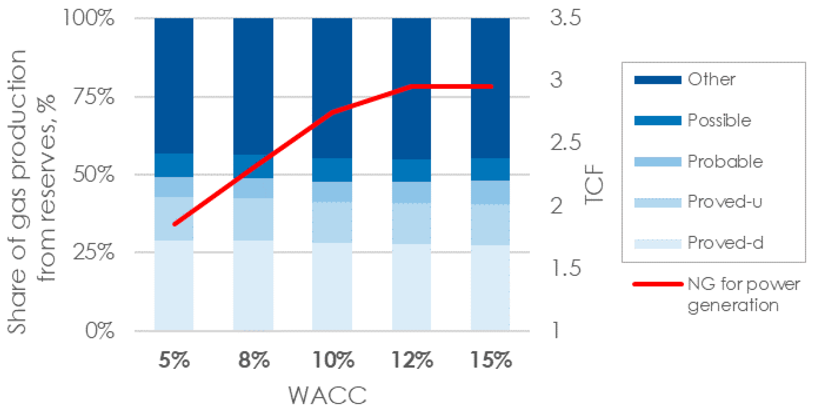
3.1.6. Opportunity Cost of Gas

Since 2001, Bolivia has subsidized gas and diesel for power generation with the aim to passing on affordable electricity prices. The subsidized gas price is equal to 1.36 US$/MMBtu for grid connected plants (Supreme Decree No. 26037 of 22 December 2000, Article 41 of the Gas Marketing Regulations. This value remains unchanged since 2001). For sake of comparison, the above price is nearly one fourth of the gas export prices to Brazil and Argentina (6.08 and 5.74 US$/MMBTU) and nearly half of the U.S. Henry Hub spot price (2.62 US$/MMBTU in 2015) [31]. The Bolivian government manages natural gas demand by setting specific prices and quotas by sector. Despite the low prices for domestic consumption, the current market structure suggests an overwhelming priority quota to exports, leaving a limited percentage of the production to the petrochemical industry. Similarly, the subsidized gas prices for gas-fueled generation disadvantage future investments in alternative energy sources. In view of such discrepancy, Bolivia require new reforms in energy prices to create a competitive gas-market. In 2004, the Supreme Decree No. 27354 explicitly called for the need of a calculation methodology that reflects the opportunity cost of using natural gas for thermoelectric generation.

“The opportunity cost” is a popular economic expression used to explain the value of foregone alternatives when evaluating a set of options. When evaluating a project, this opportunity cost represent the value of the next best alternative renounced. In our cost-minimizing model, gas exports were modelled with a ‘negative cost’ (equivalent to profit) equal to the export price.

To project gas export prices, we employ a simple econometric relation as contractual export prices are indexed to international oil prices. Our econometric relation projects natural gas prices using the WTI (West Texas International) as exogenous variable. Historical (quarterly) WTI oil prices from 1999–2015 and annual projections to 2050 (Reference Oil Scenario) were used from EIA (U.S. Energy Information Administration, Washington, DC, USA) [35]. A Vector Error Correction model estimated the long-run relationship between the WTI oil price and the gas export price. The estimated equation and relevant statistics are presented in Supplementary Materials.

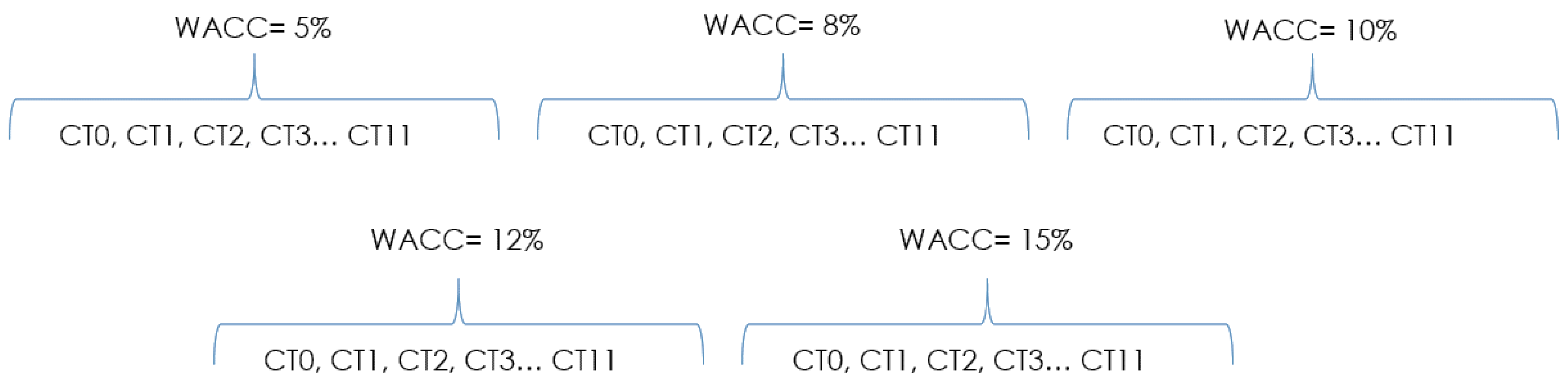
3.1.7. Discount Rate and Financial Risk

In finance, the concept of the “rate of time preference” or discount rate arises from the general observation that individuals, given the alternative, would prefer to obtain goods of value in the present rather than in the future. The opportunity cost of capital invested now is equal to the expected return of the next best alternative at the same level of risk. According to the above reasoning, the discount rate reflects the opportunity cost for the capital investment adjusted to the risk associated with the financing of said project; however, there is no definitive consensus on how to measure such costs [36,37].

The sources of financing for a project cost of capital consist of a combination of equity investors and lending institutions. In capital budgeting, the weighted average cost of capital (WACC) is used as the discount rate to define the rate that a project is expected to pay for all its capital resources [38]. WACC data from investors are scarce and respond to country-specific macroeconomic drivers, perceptions of inherent systemic risk, as well as the overall maturity of financial markets [39]. While the value of the discount rate or WACC is higher for riskier investments and lower for safer investments, developing countries have typically higher investment risks than developed countries for both, renewable and fossil-fueled power generation technologies [40,41]. The choice of the discount rate for energy systems analysis thus depends on a number of factors associated to the perceived risk and expected rate of return of the energy system.

Cost-optimization energy models such as OSeMOSYS, MESSAGE (Model of Energy Supply Strategy Alternatives and their General Environmental Impacts), MARKAL/TIMES (The Integrated MARKAL-EFOM System) and PLEXOS among others, optimize investments for energy systems and do not model the source of capital and related financing costs.

According to the Bolivian Electricity Law, the discount rate applicable to the electricity sector was set in 10% (real discount rate, adjusted for inflation) in 1994 subject to variations that may not exceed 2% [42]. No methodology or considerations of the selected discount rate are available. In 2000, the Ministry of Development Planning modified the discount rate applicable to the electricity sector by Ministerial Resolution 01/200 to 12% and has no further updates since then. The discount rate however, has an impact on system development and it may be influenced for strategic reasons—such as to move to low carbon development. This paper thus explores hypothetical discount rate scenarios that are different to the values used in the past decades. Due appropriate adjustments for opportunity costs and risk cannot be precisely estimated, sensitivity-testing scenarios were developed for comparison. A base discount rate of 12% was used and testing over a range from 5 to 15% is proposed. In total, five discount rate scenarios of 5%, 8%, 10%, 12%, and 15% are developed.

3.2. Carbon Tax Scenario Description

Carbon tax is the climate change mitigation-instrument selected in this study. In policy, it is implemented as a surcharge on fossil fuels proportional to the quantity of carbon dioxide emitted when burned. In this article, the carbon dioxide tax is levied for all fossil fuels at the point of use and it is calculated based on the carbon content of the fuel.

According to recent estimates from the 2017 Perspectives for the Energy Transition, for a scenario with a 66% chance of maintaining the temperature change below 2 °C, emissions intensity in the power sector would need to fall to around 30 gCO₂/kWh in 2050 [43]. Carbon prices that drive technological change were expected to rise in 2030 to US$120/tCO₂ in OECD countries and to US$90/tCO₂ in emerging economies for energy-related CO₂ emissions [43]. In this line, a wide selection of carbon tax scenarios with carbon prices of 0, 5, 10, 20, 30, 40, 50, 60, 70, 80, 90, and 100 US$/tCO₂ were modelled for this numerical exercise. With the aim to isolate the effect of the carbon tax in the energy system, the carbon tax was applied from 2025 and assume to continue with the same value towards 2050. The twelve scenarios were tested under five WACC scenarios described in Section 3.1.7. Thus in total, 60 scenarios were modelled as is shown in Figure 4. Note incidentally that a carbon tax would yield the same results as a ‘carbon mitigated’ subsidy for the same value. For example, a 10$/tCO₂ tax would have the same impact—in the ‘perfect market’ modelled in this analysis—as subsidy to remove carbon from the system at 10$/tCO₂. This is relevant as while should a future carbon market develop Bolivia may be eligible for a mitigation subsidies.

3.3. Metrics

Four quantitative metrics were reported to facilitate the comparison between scenarios.

3.3.1. Net Present Value (NPV)

To compare the total system costs incurred in the multiyear model period, the system NPV was the selected metric. It was calculated by the sum of the discounted cash flows of all cost streams of the power sector (capital, fixed and variable O&M, and fuel costs) for each year of the modelling period. Emissions tax penalties/revenues were excluded in this metric calculation, as seen in Equations (1) and (2):

$$NP{V}_{S,i}={\displaystyle \sum }_{t=2013}^{2040}\frac{{(I_t+OM{F}_t+OM{V}_t+F_t-S{V}_t)}_{S,i}}{{\left(1+r\right)}^t}$$

(1)

$$I=\mathrm{Overnight}\mathrm{capital}\mathrm{cost}·{\displaystyle \sum }_{t=0}^{t=yc}{\left(\begin{array}{c}\% \mathrm{Investment}\\ \mathrm{during} \\ \mathrm{construction}\end{array}\right)}_t·{\left(1+IDC\right)}^t; IDC=r$$

(2)

where: S, i refers to the scenario of interest, I_t are the investment expenditures in year t for all technologies, OMF_t and OMV_t are the fixed and variable operational and maintenance costs for all technologies in year t, F_t are the fuel costs in year t, SV_t is the salvage value of technology t at the end of the modelling period, r, the discount rate or WACC, yc, the power plant years of construction and IDC is the interest during construction, which has been assumed to be equal to the discount rate. Assumptions in spending profiles for all technologies are detailed in Table S4 in Supplementary Materials.

3.3.2. Average Carbon Intensity, CI

To compare the average CO₂ eq. emitted per unit of electricity generated in the modeling period, the average carbon intensity was calculated for each scenario, S_i as in Equation (3). To account the emissions of the energy system, emission factors per energy content were inserted to all extraction technologies and it was assumed that all fuel extracted would be burned [44].

$$C{I}_{S,i}=\frac{{\left[{\sum }_{t=2013}^{2040}{\begin{array}{c}\mathrm{Power} \mathrm{system}\\ \mathrm{Emissions}\end{array}}_t\right]}_{S,i}}{{\left[{\sum }_{t=2013}^{2040}\mathrm{Total}\mathrm{generation}\right]}_{S,i}}$$

(3)

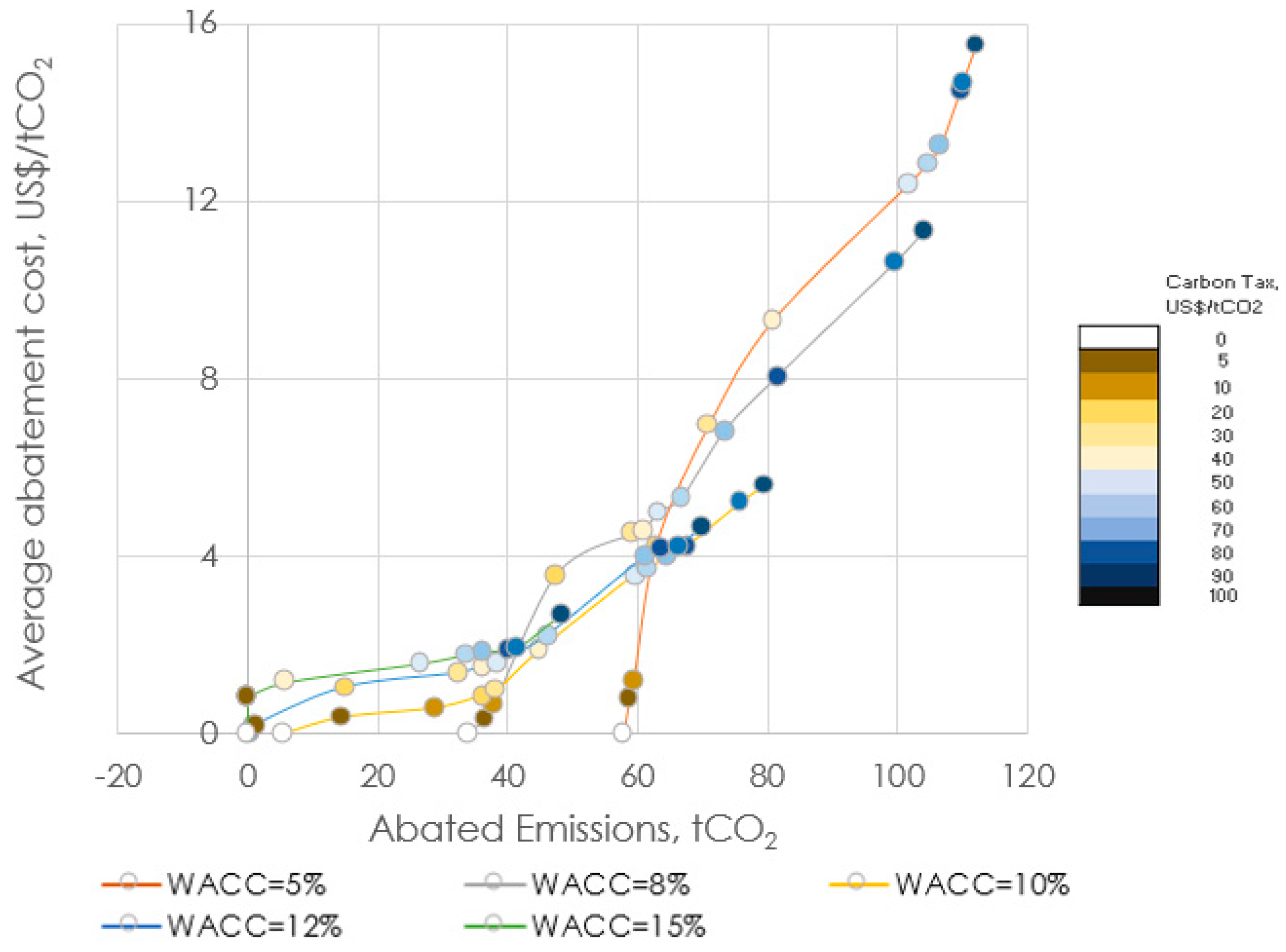
3.3.3. Average Marginal Abatement Costs (MAC)

The average marginal abatement cost MAC_S,i calculates the additional present value of the energy system per unit of avoided emissions given a carbon tax. According to the literature, the carbon abatement cost is calculated by dividing the incremental present value of the power system costs of the scenario of interest, S_i, compared to the scenario of reference, S_Ref by the avoided GHG emissions, as seen in Equation (4) [45].

$$MA{C}_{S,i}=\frac{NP{V}_{S,i}-NP{V}_{S,Ref}}{{\left[{\sum }_{t=2013}^{2040}{\begin{array}{c}\mathrm{Power} \mathrm{system}\\ \mathrm{Emissions}\end{array}}_t\right]}_{S,Ref}-{\left[{\sum }_{t=2013}^{2040}{\begin{array}{c}\mathrm{Power} \mathrm{system} \\ \mathrm{Emissions}\end{array}}_t\right]}_{S,i}}$$

(4)

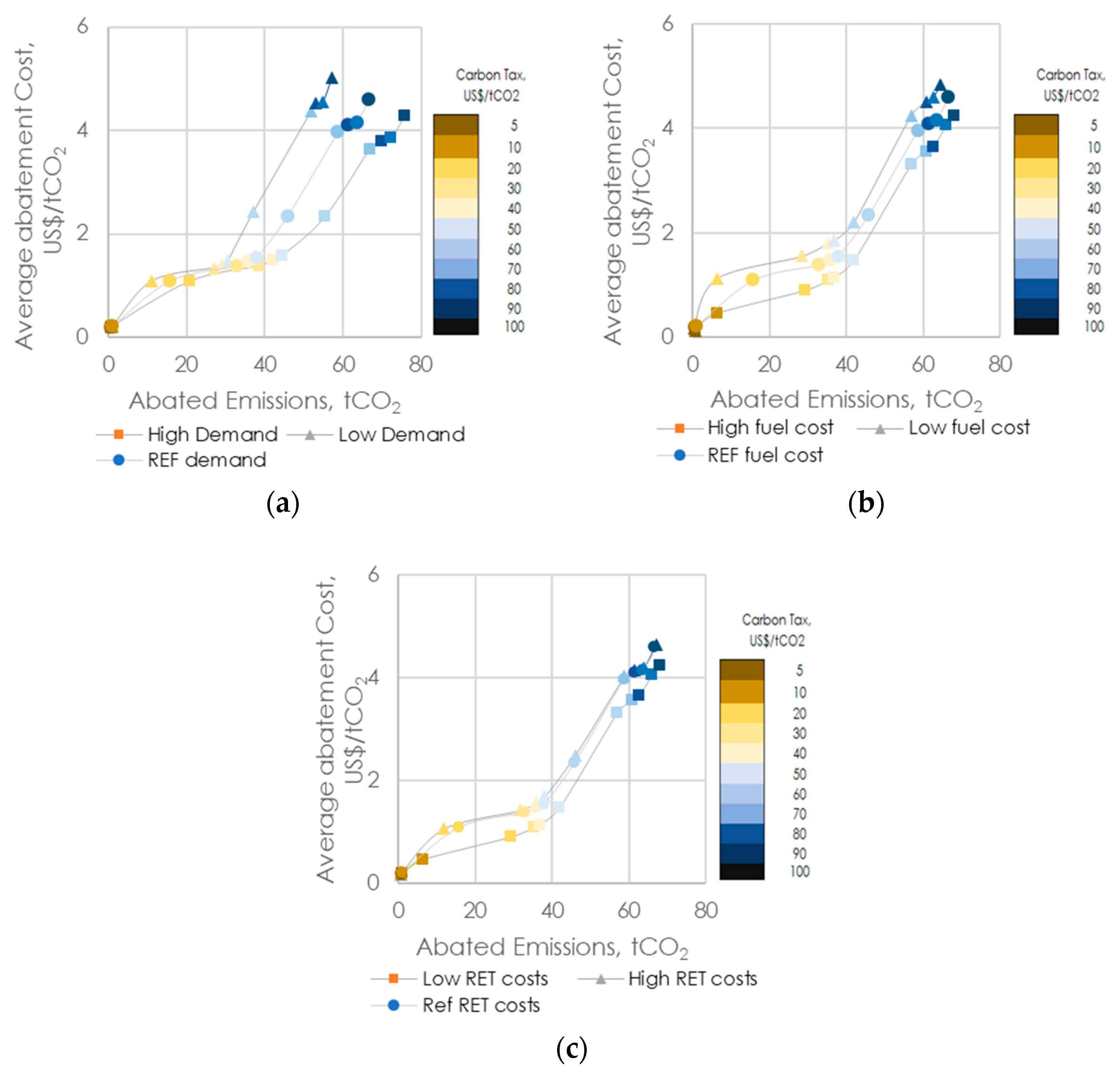
3.4. Sensitivity Analysis

The model optimization results depend on a large set of empirical data, assumptions and projections. A sensitivity analysis was thus performed on key input assumptions to assess how variations affect the optimization results when compared to the reference scenario. Due to uncertainty associated with projections, two additional scenarios, high and low, were defined for three selected key parameters: electricity demand, fuel costs, and RET costs. Learning curves (also known as experience curves) are based on the empirical observation that the unit cost of RET declines along with increased production from manufacturers. Projections and scenarios of future technology cost from the World Energy Outlook, were used in this study [2]. The assumptions considered are described in

Table 2. Reference and boundary scenarios for the parameter sensitivity analysis.

Parameter	Scenarios	Description
Demand	High and Low	From 2025–2040 two demand scenarios, high and low, were aligned with +10% and −10% of the reference electricity demand.
Fuel costs	High and Low	Variations in +10% and −10% in natural gas production costs (fixed and variable costs) were proposed for a high and low price scenario.
Renewable technologies costs	High and Low	Based on scenario assumptions (high and low) from economic learning curves from the International Atomic Energy Agency [2]. No efficiency improvements were included. Renewable technologies included: wind, solar PV, residential PV, CSP, biomass and geothermal.

. MACC were draft for each scenario. A total of 72 simulations were performed.

3.5. Modelling Platform

OSeMOSYS is an open source, bottom-up and multi-regional energy system modeling framework that uses linear and non-linear programming (LP and MILP) techniques to minimize the present value of the energy system costs to meet an exogenously defined energy demand [46]. While simplifying some of the dynamics underlying energy systems, the linear structure allows OSeMOSYS to analyze relatively complex, long term scenarios with reduced computational efforts. From this we do not derive predications, but draw insights in the form of policy relevant metrics. The code is written in a free and open source software GNU Mathprog—a part of the GNU linear programming kit (GLPK) developed to solve large scale LP problems. The model generated for this analysis is composed of 87 technologies and 48 time-slices per year.

4. Results

This section presents the results from the analysis in three separate sub-sections. First, results from the discount rate scenarios followed by the results from the different carbon tax scenarios and the parameter sensitivity analysis.

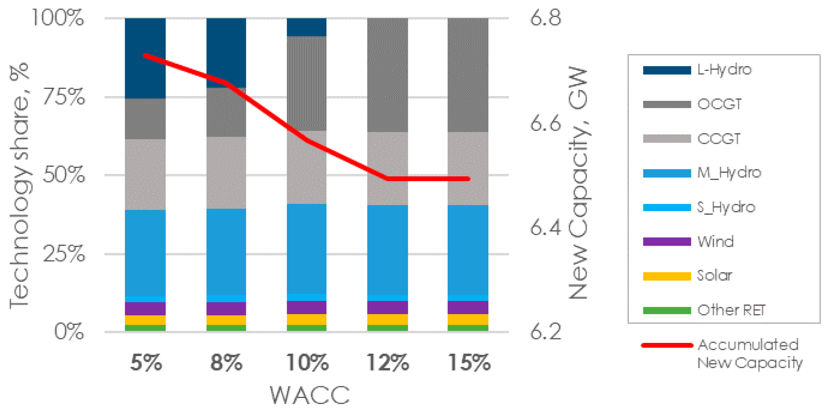
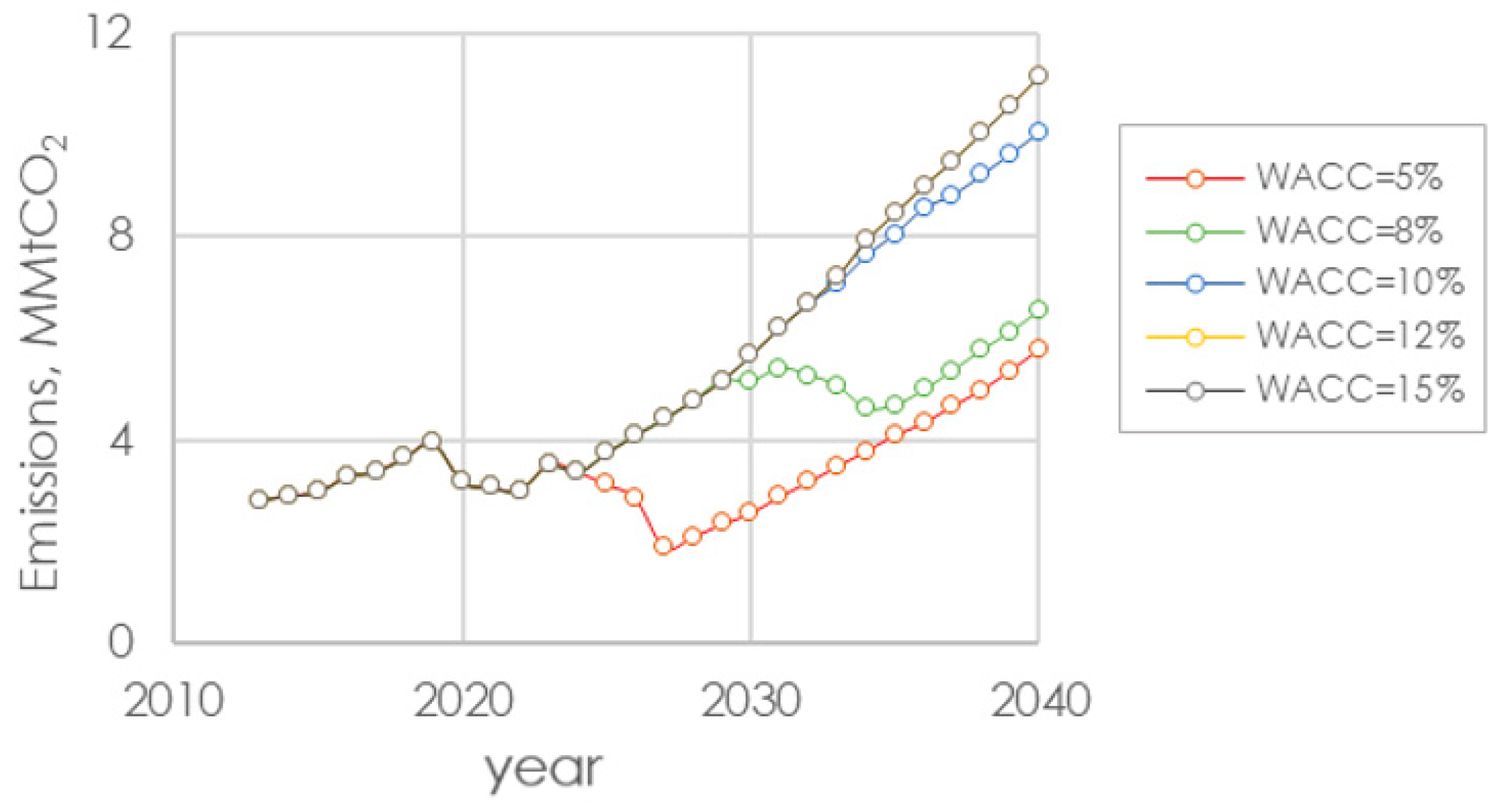
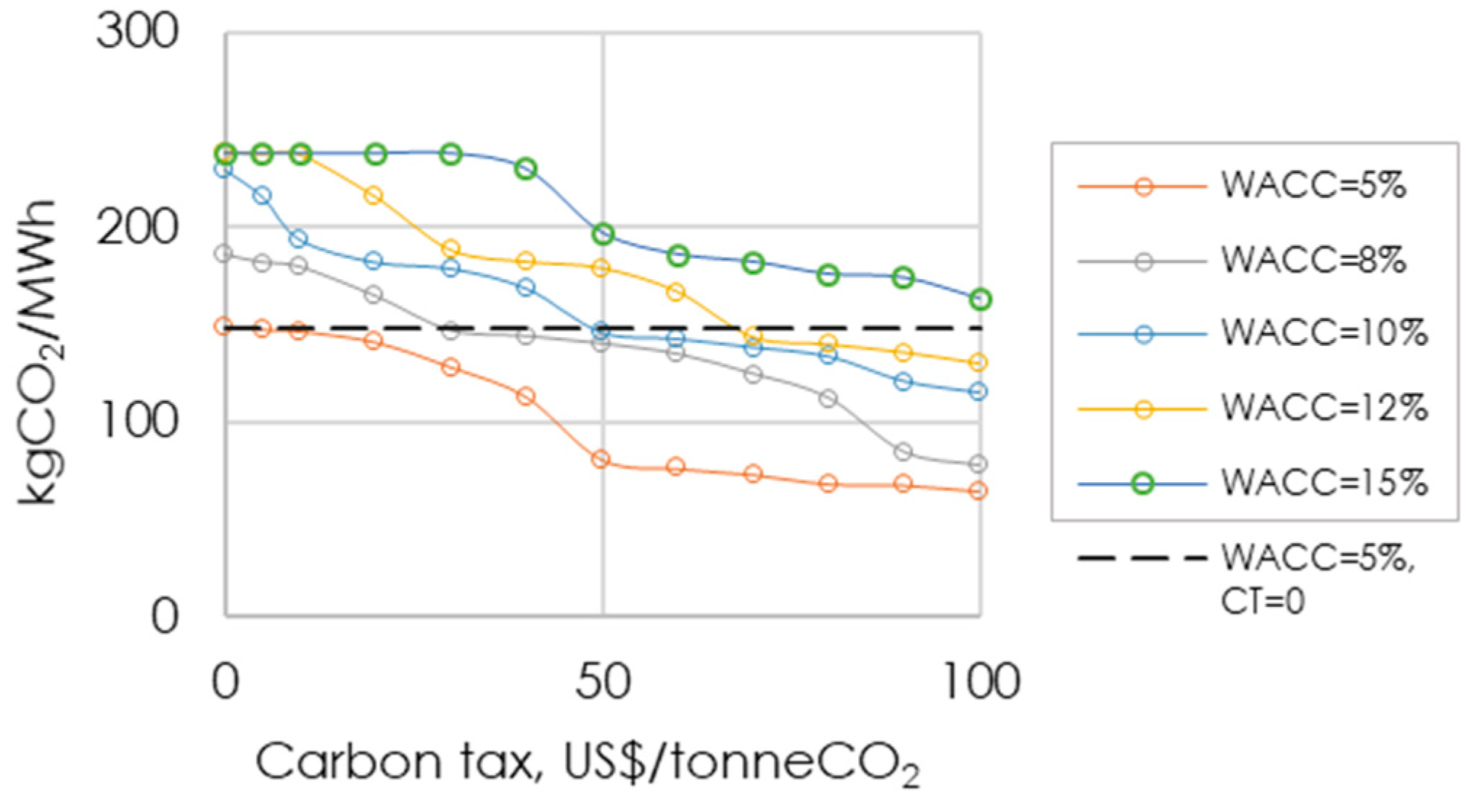
4.1. Discount Rate Scenarios

Medium-term committed projects [20,21] on medium-sized hydropower (1850 MW), small-scale hydropower (147 MW), gas combined cycle (1516 MW), wind power (267 MW), solar PV (220 MW), and other renewable projects (150 MW) are sufficient to supply the projected demand up to 2025 (these are committed and thus ‘forced’ into the solution). From 2026 onwards, new investments in additional capacity are needed year by year to supply the increasing demand.

We expect new uncommitted investment choices to vary with the WACC. Life cycle costs of RET are more sensitive to variations in the WACC due heavier upfront capital costs compared with technologies dominated by fuel costs. Consistent with the previous reasoning, Figure 5 shows the accumulated new investments by technology for the WACC scenarios. Committed new investments up to 2025 shown invariant among all scenarios. With lower values (5%, 8% and 10%) large hydro (with no fuel costs, but high up-front capital) is invested in. However, with higher values (12% and 15%) and combined with low gas costs, it becomes economical to increase the load factor of old and invest in new gas power plants. Illustrated as a solid red line, the total accumulated new capacity decreases when increasing the WACC.

Figure 6 compares the accumulated new investments in transmission capacity of high and extra-high voltage. The blue-scaled colors represent the transmission lines in each node, the red-scaled colors the transmission lines between nodes, the yellow-scaled colors the transmission lines to connect each node with the near off-grid systems and the gray-scaled colors the extra-high voltage transmission connecting strategic large-hydropower projects to the nearest node. The scenarios that insert large-scale hydropower plants (5%, 8% and 10% WACC) have a higher share of new transmission lines connecting between-nodes than the scenarios that only expand their capacity with gas-fueled technologies (12%, 15% WACC). The solid red line in Figure 6 illustrates the differences in new transmission capacity. The scenarios with 5% WACC have 1.7 GW of additional transmission capacity compared to the 12% and 15% WACC scenarios. The deployment of large-hydropower mobilizes further investments for between-node interconnection, while at the same time, reduces transmission investments in each node.

Due to a gradual increase in natural gas domestic demand, natural gas exports, and the continuous reliance on gas for power generation, 1P-2P-3P gas reserves decline fast. From 2025, Bolivia will start investing in new gas reserves, relying completely on such reserves from 2038 onwards. Figure 7 compares the investment in gas natural production for the entire energy system. The solid red line compares the natural gas used for power generation. The 5% WACC scenario consumes 1.1 TCF of natural less than the 12% and 15% WACC scenarios.

For all scenarios power generation emissions increase continuously from 7.5 MMtCO₂/year in 2013 to 15.6, 16.4, 19.9, 20.5 and 21.4 MMtCO₂/year in 2040 for 5%, 8%, 10%, 12%, and 15% WACC scenarios respectively, as seen in Figure 8. No difference in annual emissions was found between the 12% and 15% WACC scenarios.

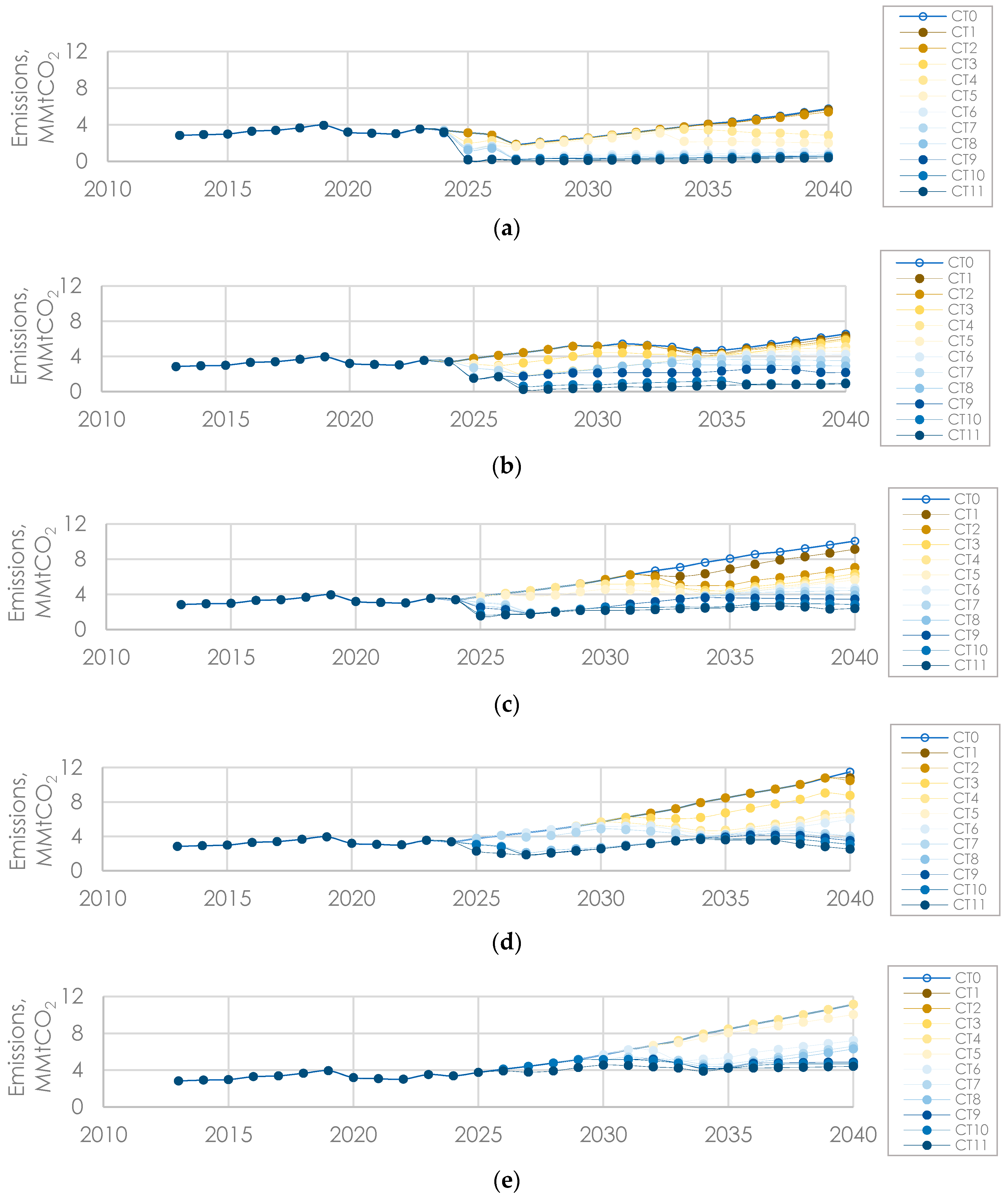
4.2. Carbon Tax Scenarios

In this section we investigate the effects of CO₂ taxes. Of interest are the levels of CO₂ that is mitigated; changes in the Bolivian system that underpin the mitigation and the resulting changes in the cost of the system. This is done for each of five WACC scenarios.

As described in the previous section, the higher the WACC, the higher the costs and capital expenditures that occur in the early years as compared to those incurred during the lifetime of the project. For this reason, renewable technologies with higher upfront capital costs become economic if the WACC is low. With increasing carbon taxes, the competitiveness of thermal generation options against RET is lowered; the degree of this is influenced by the WACC.

Figure 9 illustrates the variation of the average carbon intensity with carbon tax for all the WACC scenarios. Each point in the diagram represents a single simulation with averaged values for a multiyear period. When no carbon tax is levied, the average carbon intensity of the 5% WACC scenario is 148 kgCO₂/MWh. This is the lowest among all the other WACC scenarios due its higher inclusion of large-scaled hydropower. Values close to this are obtained when applying a carbon tax of 30, 50, 70 and more than 100 US$/tCO₂ to the 8%, 10%, 12% and 15% WACC scenario respectively (dashed line in Figure 9).

Significant reductions can be obtained when carbon emitting generation become more expensive and carbon-free generation become economically competitive. These fuel switch reductions in carbon intensity are observed in the range of 40–50 US$/tCO₂ for the 5%, 10% and 15% WACC curves while in the rage of 20–30 US$/tCO₂ for the 8% and 12% WACC curves (we don’t further develop on correlation between these values.). At the identified carbon price ranges, the CO₂ emission abatement (and consequent rapid carbon intensity improvement) is caused by fuel switching of gas fired units to large-scale hydropower deployment in the North node (in the North node, El Bala have the highest hydropower capacity factor (avg. 0.87) compared to other identified hydropower projects) [17]).

After fuel switches to large-scale hydropower, relatively smaller decrements in carbon intensity are obtained. This is observed in the range of 50–100 US$/tCO₂ for the 5%, 10%, and 15% WACC scenario, 30–80 US$/tCO₂ for the 8% and 30–60 US$/tCO₂ for the 12% WACC scenarios. At these carbon-tax and WACC ranges, the CO₂ emission abatement is caused by solar PV and wind energy investments.

For all scenarios, the overall costs and technology-specific abatement can vary significantly depending on the timing of investments. At high CO₂ emissions costs, committed projects in CCGT installed in the period 2013–2025 are phased out partially or completely before the completion of their economic lifetime. Since variations in the carbon intensity do not give information of the cost-effectiveness of carbon taxation, abatement costs were calculated for each scenario.

For each discount rate setting, a single MACC was plotted to compare the carbon abatement cost of the system given a carbon tax against the model-period abated emissions, as seen in Figure S4 in Supplementary Materials. Figure 10 compares in a single graph the average abatement costs of the system given a carbon tax scenario (y-axis) against the emission reductions of each scenario compared to the reference scenario (x-axis). In view that the discount rate influence the magnitude of present values of future cash flows, these MACC do not aim to provide numerical values of abatement costs. Yet, our analysis aims to provide a comparative visualization of the abatement costs and abated emissions for a set of carbon prices.

Due differences in technology selection between discount rate scenarios described in Section 4.1, scenarios with lower WACC than the reference scenario have immediate abated emissions when no carbon tax is applied. Similarly to the previous analysis, we can identify a carbon tax in which significant emissions reductions are obtained with the smaller increase in carbon abatement costs. The larger abated emissions per unit of abatement cost occur at carbon tax of 50 US$/tCO₂ for the 5% DR scenario, 40 US$/tCO₂ for the 8% DR scenario, 20 US$/tCO₂ for the 10% DR scenario, 30 US$/tCO₂ for the 12% DR scenario and 80 US$/tCO₂ for the 15% DR scenario.

Figure 11 illustrates the power system annual emissions for all carbon tax scenarios. Since the carbon tax is levied from 2025 onwards, different patterns are found when increasing the carbon price from 2026 onwards. When comparing the emissions level in 2040 between a scenario with no carbon tax with a scenario with the highest carbon tax (100 US$/tCO₂), we can observe different response depending of the WACC. If we compare the emission reduction the first year that the highest carbon tax is levied, an annual emission reduction of 94% is obtained for 5% WACC scenario, 59% for 8% WACC scenario, 57% for 10% WACC scenario, 51% for 12% WACC scenario, and 5% for 15% WACC scenario. The lowest the discount rate, the faster response of the energy system to carbon taxation.

4.3. Parameter Sensitivity Analysis

In this section, we present the results of the parameter sensitivity analysis for the Marginal Abatement Cost Curve (MACC) using 12% WACC to variations in electricity demand projections, natural gas production costs and RET costs. Figure 12 compares the MAC curves between the reference scenario and the alternative high and low scenarios described in Section 3.3.

Additional electricity demand requires installing additional capacity, while a lower demand is covered longer time with committed projects installed in the period 2013–2025. Smaller carbon abatement and higher abatement costs thus result for a lower demand scenario. Conversely, higher carbon abatement and lower abatement costs are expected for a high demands scenario. The largest quantity of abated emissions per unit of abatement cost occur at carbon tax of 30 US$/tCO₂ for the three demand scenarios. (Of course, lower demand results in lower absolute emissions—which is beneficial. Future work would do well to focus on energy efficiency as an option.)

Turning our focus to natural gas costs—the transition into renewable energy is slower when low fuel costs are used. It has lower abated emissions and higher carbon abatement costs. Conversely, a high fuel cost scenario allows a faster transition into renewable energy with higher abated emission and lower abatement costs. The largest quantity of abated emissions per unit of abatement cost occur at carbon tax of 30 US$/tCO₂ for the three natural gas production scenarios.

For third parameter sensitivity scenario, little difference (less than 2%) is found between the low RET costs scenario and the Reference scenario. However, lower RET costs allow a higher insertion of solar and wind energy with higher abated emissions and lower carbon abatement costs. As with the other scenarios, the largest amount abated emissions per unit of abatement cost occur at carbon tax of 30 US$/tCO₂ for the three natural RET cost scenarios.

5. Discussion

The methodology presented in this article evaluates the effect of the WACC on MACC when applying carbon taxation to the power generation sector. Results obtained are based on numerical methods and a set of assumptions and do not aim to predict the evolution of the power sector in Bolivia. The article presents various, and limited insights for potential configurations of, emissions from and CO₂ taxes on the Bolivian electricity system.

Our numerical estimates support a consistent finding, the emission reduction effect of carbon pricing is undermined when the WACC is high. This premise is supported with the values obtained in our assessment which are well in the range of estimates of comparable work from Hirth et al., Van den Bergh et al. and Soloveitchik et al. [12,41,47]. Hirth et al. performed a numerical exercise estimating reductions in carbon intensity of power generation with carbon prices in the rage of 0–100 US$/tCO₂ and WACC in the range of 0–25% are applied. Their estimates suggest that WACC needs to be reduced to levels lower than 5% to produce at least 30 percent electricity from renewable energy sources [41]. Van den Bergh et al. estimated a curve to relate CO₂ cost and wind energy investments in Central West Europe. Investments in wind were found to be triggered as of a CO₂ cost higher that 35 EUR/tCO₂ [12]. Finally Soloveitchik et al. estimated the multi-year period MACC for the Israeli power generation system when carbon taxes in the range from 5–50 US$/tCO₂ are applied. For the period 2001–2013 a carbon abatement cost of 19.5 US$/tCO₂ and emission reduction of 7.7% are achieved when a carbon price of 50 US$/tCO₂ is applied.

Our results clearly come with a number of caveats. Shortcomings in robustness in MACC have been also addressed in the literature by Delarue, Kesicki and Stranchan, Kesicki and Ekins and Van den Berg, among others [9,12,48,49]. We remark on the importance of uncertainty in the costs and abatement potentials estimates, constant updates, and careful assessment are required to derive policy implications. However, we note that there are important ranges and combinations of carbon tax/mitigation potential/discount rate to consider when designing policy. Critical among these are the dynamics associated with discount rate and ease of CO₂ mitigation. On the other hand, higher financing costs secure domestic gas consumption.

Carbon taxes represent a cost-effective policy instrument to impose on the vast heterogeneity of GHG individual emitters, provide a continuous incentive for adoption and innovation of carbon efficient technologies, are simpler to administer and do not draw upon government budgets [50]. Despite these advantages, to date, the implementation of carbon taxes worldwide has been limited [3]. The success of carbon taxation depends on a wide list of factors that need to be revised. Carattini et al. and Baranzini et al. identified barriers to public acceptance of carbon taxes, underlining the importance of proper policy design coupled with communication on the effects of carbon taxes [51,52]. The literature acknowledges a series of unwanted effects of carbon taxes on distribution of income (heavier burden in the lower income groups) and competitiveness (production costs rise). Based on a review of empirical studies on existing carbon taxes, Zhang et al. concluded that competitive losses are not significant and distributive impacts may need in future to incorporate the distribution of benefits from improved environment quality [53]. Shah and Larsen argue that carbon taxes can raise significant revenues in developing countries with effective tax systems to partially compensate for corporate income taxes and, not likely to have a regressive impact as commonly perceived [54].

Results from our study illustrate that high capital costs, expressed as high WACC, tend to encourage the use of fossil fuels and undermine the effectiveness of carbon pricing. Comparably, in a study of the effect of financing costs and the solar resource on the levelized cost of solar PV power, Ondraczek et al. found that variations in the WACC have more important influence than variations in solar radiation [39]. The importance of adequate financing instruments for the future success of RET have been also recognized by a recent article from Creutzig et al. [55]. Hirth and Steckel demonstrated using a numerical example that high capital costs (high WACC) can significantly reduce the decarbonization effect of carbon prices [41].

WACC for power generation technologies widely differ between developed and developing countries. For example, WACC for solar PV in Japan (3.7%), Switzerland (3.9%) and the U.K. (4.1%) are very low when compared to Madagascar (29%), Brazil (28.4%), and Congo DR (21.4%) [39]. Among others, access to capital and systemic risks in the market contribute to such differences on investor’s risk perception between countries [56,57].

Few studies identifying the reasons and possible solutions for de-risking renewable energy investment are available in literature. Steckel and Jakob outlined a number of policies that could be employed to de-risk investments at national and international level and hence make investment into capital intensive low-carbon technologies more attractive [58]. Stable and transparent policy environments, political economy of distribution, robust policy design and financial de-risking support for private investments are outlined. Similarly, a methodology developed by the United Nations Developing Program shows that cost of equity and costs of debt can be reduced by using identified de-risking instruments for nine identified risk categories which are: power market, permits, social acceptance, resource and technology, grid-transmission, counterparty, financial-sector, political, and macroeconomic risk [40].

Reducing financing costs for RET investments in developing countries with untapped renewable potential represent an opportunity for policy makers to prompt private investment. Unfortunately, in many developing countries such as Bolivia, financial de-risking is still provided to gas-fired generation (through fuel subsidies), which exacerbates existing difficulties to finance RET (in effect, these subsidies are equivalent to a negative emissions price). Removing this bias against low-carbon energy sources is required as a first step to implement effective climate change mitigation policy [58]. Additionally, studies on financial de-risking instruments are required to identify which drivers have greater potential to reduce the WACC and more important, studies about the cost-effectiveness of reducing the WACC are required.

6. Conclusions

Though limited, this analysis deepens the insights of the relation between carbon tax, discount rate, abated emissions and abatement costs. The methodology is illustrated with a detailed bottom-up least-cost optimization model of the power sector of Bolivia with country-specific data. For our specific case study, using a 12% WACC, we found that a carbon tax of 30 US$/tCO₂ produces the larger abated emissions per unit of abatement cost. We identify a number of ranges (relating the WACC to emissions reductions and associated costs) that will be of importance for designing mitigation policy in Bolivia. Results from our study are based on a set of country-specific assumptions and simplifications. Nonetheless, the methodology can be replicated to other study cases to assess early stages of carbon pricing initiatives and contribute to ongoing negotiations of international protocols for emissions mitigation.

References

1. IPCC. Climate Change 2014; Synthesis Report. Contribution of Working Groups I, II and III to the Fifth Assesment Report of the Intergovernmental Panel on Climate Change; Core Writing Team; Pachauru, R.K., Meyer, L.A., Eds.; IPCC: Geneva, Switzerland, 2014. [Google Scholar]
2. International Energy Agency. World Energy Outlook 2016; International Energy Agency: Paris, France, 2016. [Google Scholar]
3. Goyal, R.; Gray, S.; Kallhauge, A.C.; Nierop, S.; Berg, T.; Leuschner, P. State and Trends of Carbon Pricing 2018; The World Bank: Washington, DC, USA, 2018. [Google Scholar]
4. Zachariadis, T. Proposal for a Green Tax Reform in Cyprus. Cyprus Econ. Policy Rev. 2016, 10, 127–139. [Google Scholar]
5. IRENA. The Power to Change: Solar and Wind Cost Reduction Potential to 2025; IRENA: Abu Dhabi, UAE, 2016. [Google Scholar]
6. Schmidt, T.S. Low-carbon investment risks and de-risking: Nature Climate Change: Nature Research. Nat. Clim. Chang. 2014, 1, 237–239. [Google Scholar] [CrossRef]
7. Ellerman, A.D.; Decaux, A. Analysis of Post-Kyoto CO2 Emissions Trading Using Marginal Abatement Curves. Available online: http://web.mit.edu/globalchange/www/MITJPSPGC_Rpt40.pdf (accessed on 10 October 2018).
8. Criqui, P.; Mima, S.; Viguier, L. Marginal abatement costs of CO2 emission reductions, geographical flexibility and concrete ceilings: An assessment using the POLES model. Energy Policy 1999, 27, 585–601. [Google Scholar] [CrossRef]
9. Kesicki, F.; Strachan, N. Marginal abatement cost (MAC) curves: Confronting theory and practice. Environ. Sci. Policy 2011, 14, 1195–1204. [Google Scholar] [CrossRef]
10. Huang, S.K.; Kuo, L.; Chou, K.-L. The applicability of marginal abatement cost approach: A comprehensive review. J. Clean. Prod. 2016, 127, 59–71. [Google Scholar] [CrossRef]
11. Gollop, F.M.; Roberts, M.J. Cost-Minimizing Regulation of Sulfur Emissions: Regional Gains in Electric Power. Rev. Econ. Stat. 1985, 67, 81–90. [Google Scholar] [CrossRef]
12. Van den Bergh, K.; Delarue, E. Quantifying CO2 abatement costs in the power sector. Energy Policy 2015, 80, 88–97. [Google Scholar] [CrossRef]
13. Intended Nationally Determined Contribution from the Plurinational State of Bolivia. Available online: http://www.planificacion.gob.bo/uploads/4.BOLIVIA_INDC_ENGLISH.pdf (accessed on 10 October 2018).
14. Comité Nacional de Despacho de Carga. Generation and Transmission Capacity Bolivia. 2017. Available online: https://www.cndc.bo/agentes/generacion.php (accessed on 15 July 2018).
15. USGS. Hydropower Assessment of Bolivia—A Multisource Satellite Data and Hydrologic Modeling Approach; USGS: Reston, VA, USA, 2016.
16. Coady, D.; Parry, I.W.; Sears, L.; Shang, B. How Large Are Global Energy Subsidies? Working Paper No. 15/105; International Monetary Fund: Washington, DC, USA, 2015; p. 42. [Google Scholar]
17. Ministry of Hydrocarbons and Energy. Plan Eléctrico del Estado Plurinacional de Bolivia 2015–2025; Ministry of Hydrocarbons and Energy: La Paz, Bolivia, 2014.
18. Plurinational State of Bolivia. Plan de Desarrollo Economico y Social 2016–2020. Available online: http://www.planificacion.gob.bo/uploads/PDES_INGLES.pdf (accessed on 10 October 2018).
19. Countries in Latin American and the Caribbean Region Leading Climate Action. Available online: https://unfccc.int/news/countries-in-latin-american-and-the-caribbean-region-leading-climate-action (accessed on 10 July 2018).
20. Balderrama, J.G.P.; Broad, O.; Sevillano, R.C.; Alejo, L.; Howells, M. Techno-economic demand projections and scenarios for the Bolivian energy system. Energy Strategy Rev. 2017, 16, 96–109. [Google Scholar] [CrossRef] [Green Version]
21. Comité Nacional de Despacho de Carga. Plan de Expansión del Sistema Interconectado Nacional; Comité Nacional de Despacho de Carga: Cochabamba, Bolivia, 2012. [Google Scholar]
22. ENDE Coorporación. Proyectos en Estudio. Available online: http://www.ende.bo/proyectos/estudio (accessed on 11 July 2017).
23. Autoridad de Electricidad. Anuario Estadistico 2015; Autoridad de Electricidad: Cochabamba, Bolivia, 2015. [Google Scholar]
24. Yacimientos Petrolíferos Fiscales Bolivianos. Plan Estratégico Corporativo (PEC) 2015–2019; Yacimientos Petrolíferos Fiscales Bolivianos: La Paz, Bolivia, 2014. [Google Scholar]
25. EIA. Technically Recoverable Shale Oil and Shale Gas Resources; EIA: Washington, DC, USA, 2015.
26. USGS. Assessment of Undiscovered Conventional Oil and Gas Resources of South America and the Caribbean; World Petroleum Resources Project; USGS: Reston, VA, USA, 2012.
27. Ministerio de Hidrocarburos y Energía. Balance Energético Nacional 2000–2013; Ministerio de Hidrocarburos y Energía: La Paz, Bolivia, 2014.
28. Boletín Estadístico Gestión 2013. Available online: http://www.cedla.org/sites/default/files/Boletin%20Estadistico%20Enero%20Diciembre%202013.pdf (accessed on 10 October 2018).
29. Pfenninger, S.; Staffell, I. Long-term patterns of European PV output using 30 years of validated hourly reanalysis and satellite data. Energy 2016, 114, 1251–1265. [Google Scholar] [CrossRef]
30. Staffell, I.; Pfenninger, S. Using bias-corrected reanalysis to simulate current and future wind power output. Energy 2016, 114, 1224–1239. [Google Scholar] [CrossRef]
31. Agencia-Nacional-de-Hidrocarburos. Anuario Estadístico 2016; Agencia-Nacional-de-Hidrocarburos: Cochabamba, Bolivia, 2017.
32. Chávez-Rodríguez, M.F.; Garaffa, R.; Andrade, G.; Cárdenas, G.; Szklo, A.; Lucena, A.F.P. Can Bolivia keep its role as a major natural gas exporter in South America? J. Nat. Gas Sci. Eng. 2016, 33, 717–730. [Google Scholar] [CrossRef]
33. Lucena, A.F.P.; Clarke, L.; Schaeffer, R.; Szklo, A.; Rochedo, P.R.; Nogueira, L.P.; Daenzer, K.; Gurgel, A.; Kitous, A.; Kober, T. Climate policy scenarios in Brazil: A multi-model comparison for energy. Energy Econ. 2016, 56, 564–574. [Google Scholar] [CrossRef]
34. Rudnick, H.; Barroso, L.; Cunha, G.; Mocarquer, S. Electricity-gas integration challenges in South America. IEEE Power Energy Mag. 2014, 12, 29–39. [Google Scholar] [CrossRef]
35. EIA. Annual Energy Outlook. Energy Prices by Sector and Source; U.S. Energy Information Administration: Washington, DC, USA, 2016.
36. Harrison, M. Valuing the Future: The Social Discount Rate in Cost-Benefit Analysis; Productivity Comission: Melbourne, Australian, 2010.
37. Zhuang, J.; Liang, Z.; Lin, T.; de Guzman, F. Theory and Practice in the Choice of Social Discount Rate for Cost-Benefit Analysis: A Survey; Economics and Research Department, Asian Development Bank: Manila, Philippines, 2007. [Google Scholar]
38. Simshauser, P. The cost of capital for power generation in atypical capital market conditions. Econ. Anal. Policy 2014, 44, 184–201. [Google Scholar] [CrossRef]
39. Ondraczek, J.; Komendantova, N.; Patt, A. WACC the dog: The effect of financing costs on the levelized cost of solar PV power. Renew. Energy 2015, 75, 888–898. [Google Scholar] [CrossRef]
40. UNDP. Derisking Renewable Energy Investment | UNDP; UNDP: New York, NY, USA, 2013. [Google Scholar]
41. Hirth, L.; Steckel, J.C. The role of capital costs in decarbonizing the electricity sector. Environ. Res. Lett. 2016, 11, 114010. [Google Scholar] [CrossRef] [Green Version]
42. Plurinational State of Bolivia. Ley de Electricidad. Artículo 48: 1994. Available online: https://www.lexivox.org/norms/BO-RE-DS24043D.xhtml (accessed on 10 October 2018).
43. Perspectives for the energy transition: Investment Needs for a Low-Carbon Energy System. 2017. Available online: https://www.iea.org/publications/insights/insightpublications/ (accessed on 10 October 2018).
44. EIA. Carbon Dioxide Emissions Coefficients; U.S. Energy Information Administration: Washington, DC, USA, 2016. Available online: https://www.eia.gov/environment/emissions/co2_vol_mass.php (accessed on 14 February 2018).
45. Ibrahim, N.; Kennedy, C. A Methodology for Constructing Marginal Abatement Cost Curves for Climate Action in Cities. Energies 2016, 9, 227. [Google Scholar] [CrossRef]
46. Howells, M.; Rogner, H.; Strachan, N.; Heaps, C.; Huntington, H.; Kypreos, S.; Hughes, A.; Silveira, S.; DeCarolis, J.; Bazillian, M.; et al. OSeMOSYS: The Open Source Energy Modeling System. Energy Policy 2011, 39, 5850–5870. [Google Scholar] [CrossRef]
47. Soloveitchik, D.; Ben-Aderet, N.; Grinman, M.; Lotov, A. Multiobjective optimization and marginal pollution abatement cost in the electricity sector—An Israeli case study. Eur. J. Oper. Res. 2002, 140, 571–583. [Google Scholar] [CrossRef]
48. Delarue, E.D.; Ellerman, A.D.; D’haeseleer, W.D. Robust MACCs? The topography of abatement by fuel switching in the European power sector. Energy 2010, 35, 1465–1475. [Google Scholar] [CrossRef] [Green Version]
49. Kesicki, F.; Ekins, P. Marginal abatement cost curves: A call for caution. Clim. Policy 2012, 12, 219–236. [Google Scholar] [CrossRef]
50. Baranzini, A.; van den Bergh, J.C.J.M.; Carattini, S.; Howarth, R.B.; Padilla, E.; Roca, J. Carbon pricing in climate policy: Seven reasons, complementary instruments, and political economy considerations. Wiley Interdisciplin. Rev. Clim. Chang. 2017, 8, e462. [Google Scholar] [CrossRef]
51. Carattini, S.; Carvalho, M.; Fankhauser, S. Overcoming public resistance to carbon taxes. Wiley Interdisciplin. Rev. Clim. Chang. 2018, 9, e531. [Google Scholar] [CrossRef]
52. Baranzini, A.; Carattini, S. Effectiveness, earmarking and labeling: Testing the acceptability of carbon taxes with survey data. Environ. Econ. Policy Stud. 2017, 19, 197–227. [Google Scholar] [CrossRef] [Green Version]
53. Zhang, Z.; Baranzini, A. What do we know about carbon taxes? An inquiry into their impacts on competitiveness and distribution of income. Energy Policy 2016, 32, 507–518. [Google Scholar] [CrossRef]
54. Shah, A.; Larsen, B. Carbon Taxes, the Greenhouse Effect, and Developing Countries. Available online: http://documents.worldbank.org/curated/en/460851468739298164/Carbon-taxes-the-greenhouse-effect-and-developing-countries (accessed on 10 October 2018).
55. Creutzig, F.; Agoston, P.; Goldschmidt, J.C.; Luderer, G.; Nemet, G.; Pietzcker, R.C. The underestimated potential of solar energy to mitigate climate change. Nat. Energy 2017, 2, 17140. [Google Scholar] [CrossRef]
56. Painuly, J. Barriers to renewable energy penetration; a framework for analysis. Renew. Energy 2001, 24, 73–89. [Google Scholar] [CrossRef]
57. UNEPFI. Financing Renewable Energy in Developing Countries; Drivers and Barriers for Private Finance in Sub-Saharan Africa Financing Renewable Energy in Developing Countries; United Nations Environment Programme Finance Initiative: Geneva, Switzerland, 2012. [Google Scholar]
58. Steckel, J.C.; Jakob, M. The role of financing cost and de-risking strategies for clean energy investment. Int. Econ. 2018, 155, 19–28. [Google Scholar] [CrossRef]
Figure 1. Geographical representation of the energy model and sub-regional division in the current grid configuration.
Energies 11 02738 g001
Figure 2. Energy system representation.
Energies 11 02738 g002
Figure 3. Basin delineation and areas represented in the model. (a) Altiplano; (b) Amazon; (c) La Plata.
Energies 11 02738 g003
Figure 4. Scenarios modelled.
Energies 11 02738 g004
Figure 5. Accumulated new power generation capacity 2013–2040 for all WACC scenarios.
Energies 11 02738 g005
Figure 6. Accumulated new transmission capacity 2013–2040 for all WACC scenarios.
Energies 11 02738 g006
Figure 7. Accumulated natural gas production from reserves 2013–2040.
Energies 11 02738 g007
Figure 8. Power system emissions for all WACC scenarios.
Energies 11 02738 g008
Figure 9. Average multiyear carbon intensity vs. carbon tax for five WACC scenarios.
Energies 11 02738 g009
Figure 10. Average multiyear abatement costs vs abated emissions of each scenario compared to the reference scenario.
Energies 11 02738 g010
Figure 11. Annual Emissions for all discount rate and carbon tax scenarios. (a) WACC = 5%; (b) WACC = 8%; (c) WACC = 10%; (d) WACC = 12%; (e) WACC = 15%.
Energies 11 02738 g011
Figure 12. Parameter sensitivity-analysis results. (a) Electricity demand, (b) fuel production costs and (c) renewable energy technology (RET) costs.
Energies 11 02738 g012