Scavenging Ports’ Optimal Design of a Two-Stroke Small Aeroengine Based on the Benson/Bradham Model

Abstract

The two-stroke engine is a common power source for small and medium-sized unmanned aerial vehicles (UAV), which has wide civil and military applications. To improve the engine performance, we chose a prototype two-stroke small areoengine, and optimized the geometric parameters of the scavenging ports by performing one-dimensional (1D) and three-dimensional (3D) computational fluid dynamics (CFD) coupling simulations. The prototype engine is tested on a dynamometer to measure in-cylinder pressure curves, as a reference for subsequent simulations. A GT Power simulation model is established and validated against experimental data to provide initial conditions and boundary conditions for the subsequent AVL FIRE simulations. Four parameters are considered as optimal design factors in this research: Tilt angle of the central scavenging port, tilt angle of lateral scavenging ports, slip angle of lateral scavenging ports, and width ratio of the central scavenging port. An evaluation objective function based on the Benson/Bradham model is selected as the optimization goal. Two different operating conditions, including the take-off and cruise of the UAV are considered. The results include: (1) Orthogonal experiments are analyzed, and the significance of parameters are discussed; (2) the best factors combination is concluded, followed by simulation verification; (3) results before and after optimization are compared in details, including specific scavenging indexes (delivery ratio, trapping efficiency, scavenging efficiency, etc.), conventional performance indicators, and the sectional views of gas composition distribution inside the cylinder.

1. Introduction

In the context of the information age of the 21st century, unmanned aerial vehicle (UAV) technology has gradually matured with the rapid development of microelectronics technology and communication technology. Compared with manned aircrafts, UAVs are small in size, light in weight, undemanding in runway requirements, low in manufacturing and use cost, and can also reduce casualties on the battlefield. Therefore, UAVs are widespread in both military and civilian applications. Besides, small and medium-sized UAVs (maximum take-off weights of 10 to 1000 kg) are particularly popular because of good overall performance and usage convenience [1]. Pressured by increasingly stringent emission regulations, crankcase scavenged two-stroke engines are scarcely applied in the automotive industry [2]. However, benefitting from its significant advantages in simple structure, few accessories, and high power density, the two-stroke engine is universally selected as the power source of small and medium-sized UAVs. In Europe and the United States, several companies specialize in producing two-stroke light-duty engines for small and medium-sized UAVs, such as 3 W, Gobler Hirth, and Limbach in Germany, Wilksch in the UK, Zanzottera in Italy, and XRDi and DeltaHawk in the US [3].

Different from conventional four-stroke engines equipped with sophisticated valve timing systems, two-stroke engines generally employ the opening and closing of piston-motion-controlled scavenging ports as the way of pumping and exhausting. The comparatively simple scavenging system shows its superiority in engine design and manufacturing, but significant drawbacks also emerge in volumetric efficiency and in-cylinder gas flow control [4,5]. The potential of two-stroke engines has become more and more subject to increasing research work trying to optimize the gas motion during the scavenging process. The gas motion is notably dependent on the specific design of scavenging ports. Therefore, the latter is consequently selected as the research focus of this paper.

A major problem in constructing the two-stroke engine model is to describe the corresponding scavenging process. Since the first two-stroke engine at the end of 19th century by Sir Dugald Clerk, various different scavenging systems have been designed and pertinent scavenging models have been successively developed and optimized by tracking studies to draw conclusions about the quality of scavenging process. Merker and Gerstle summarized a tremendous number of scavenging models and proposed a comprehensive evaluation of existing models [6]. They classified existing models into three categories. Precision, mathematical expenditure, the structure of the formula, and the difficulty of empirical parameter calibration were all taken into account to obtain the assessment results. Ma et al. applied a relatively simple perfect displacement model and perfect mixing model in the simulation modeling method and experimental investigation on the uniflow scavenging system of an opposed-piston folded-cranktrain diesel engine [7]. Based on the single-zone Benson model, Brynych et al. proposed a way of generalizing the scavenging curves to lower the time cost of three-dimensional (3D) computational fluid dynamics (CFD) simulations and accelerated the procedure of engine optimization substantially [8]. Mattarelli et al. chose main scavenging coefficients (charging efficiency, scavenging efficiency, trapping efficiency, delivery ratio, etc.) as port design criteria for two-stroke loop scavenged engines and performed a series of multi-cycle 3D CFD simulations to validate the optimum configuration obtained from the previous parametric analysis [9]. The final results demonstrated the excellent efficiency of the scavenging process. Similarly, to fulfill the potential of boosted uniflow scavenged direct injection gasoline (BUSDIG), disparate layout schemes of scavenging ports were designed and corresponding parameters were varied to investigate their impacts on the scavenging performance and the in-cylinder gas motion [10,11,12].

In the current studies, burgeoning one-dimensional (1D)/3D simulation technologies conspire to play an important role in providing researchers with essential and powerful tools for rapid prototyping, massive data processing, and visualization analysis [13]. Regarding the optimization of the scavenging systems of two-stroke engines, simulation techniques also show promising potential and have yielded many fruitful research achievements [14,15,16]. Cui et al. conducted a detailed CFD analysis of the scavenging process in a steady-state scavenging flow test and adopted the proper orthogonal decomposition (POD) method in search of the cause of precession phenomenon found in the high swirl model [17]. Xie et al. performed the numerical simulation of an Opposed-Piston 2-Stroke Diesel Engine (OP2S) and compared the results of in-cylinder gas motion with those of a uniflow-scavenged two-stroke engine using CFD engine models [18]. Zang et al. investigated the scavenging process of Linear Internal Combustion Engine-Linear Generator Integrated System (LICELGIS) and implemented a steady-state verification test to further explore the motion characteristics of LICELGIS [19]. Mattarelli et al. reported a CFD study on a two-stroke Opposed Piston High Speed Direct Injection Diesel Engine (OPHSDI) and analyzed the influence of the offset between the crankshafts by performing 3D CFD simulations [20]. Li et al. investigated the influences of intake ports and pent-roof structures on the flow characteristics of a poppet-valved two-stroke gasoline engine to minimize the short-circuiting of the intake charge [21]. He et al. emphasized the significant effects of exhaust back pressure, porting timing, and intake port layout on the scavenging quality and trapped air mass in cylinder by transient CFD simulation, including blow-down and scavenging [22]. Zhou et al. performed the thermodynamic simulation of a self-balanced opposed-piston folded-cranktrain two-stroke engine for UAVs to improve engine performance indicators, including power density, fuel compatibility, fuel economy, and durability in a harsh environment [23].

The scavenging process is the key for in-cylinder gas motion and the mixing of fresh air and injected fuel, which has remarkable influence on the in-cylinder combustion process and, eventually, on the engine performance. However, relevant two-stroke engine scavenging system optimization schemes proposed in previous studies were scarcely targeted from the perspective of scavenging models. Instead of considering comparatively sophisticated scavenging models, such as the Dang/Wallace model and Benson/Bradham model, previous researchers usually employed conventional scavenging evaluation indexes (charging efficiency, scavenging efficiency, trapping efficiency, deliver ratio, etc.) as the evaluation criteria of scavenging ports’ optimal design [6]. For the deeper investigation of the scavenging process, a two-stroke small aeroengine is selected as the prototype. Afterwards, the geometric structure of the prototype engine is parameterized. An objective function based on the more comprehensive Benson/Bradham model is established in this paper. To guarantee the consistency and compatibility between 1D and 3D boundary conditions, a 1D/3D coupling numerical simulation architecture is set up and validated against the prototype experimental data. Commonly, 3D CFD simulation is a time-consuming process on the condition that all the possible combinations of geometric parameters need to be traversed. By varying the parameters, the number of investigated cases amounted to 1352 along with dramatically increasing the time expenditure [9]. To minimize the time cost of determining the most effective geometric parameters configuration, the orthogonal experimental design (OED) method is employed to reduce the 3D CFD simulation amount. Additionally, optimization results are validated by performing dedicated 3D CFD simulations. The objective function value, scavenging indexes (delivery ratio, trapping efficiency, scavenging efficiency, etc.), conventional performance indexes, including the indicated mean effective pressure (IMEP) and indicated specific fuel consumption (ISFC), and the sectional views of gas composition distribution inside the cylinder are all taken into consideration when comparing results before and after the optimization.

2. Scavenging System Modeling

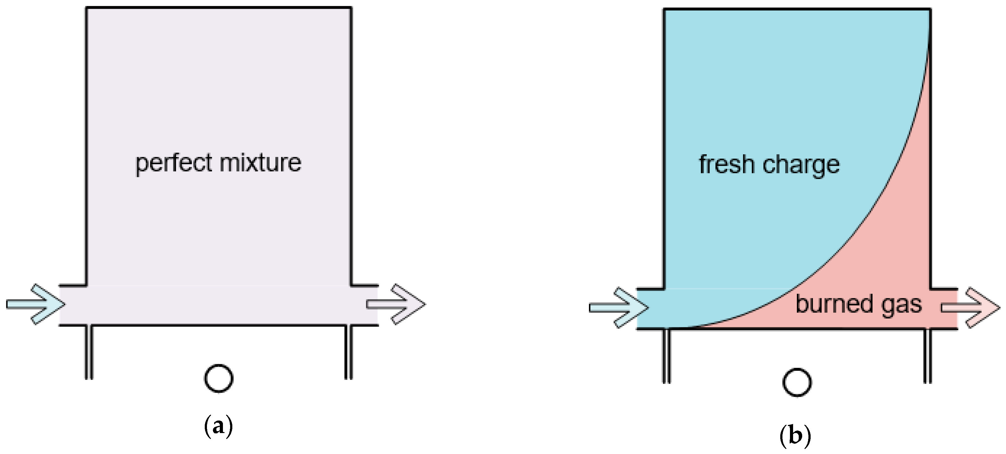
2.1. Scavenging Model Selection

Quantitative evaluation indexes are needed to describe the quality of the scavenging process of a two-stroke engine. Corresponding mathematical models abstracted from an actual scavenging process can serve for this purpose and reflect how much fresh charge can be delivered and trapped in the cylinder through specific model parameters [24,25]. To establish the scavenging model, several mass parameters are defined as follows: $m_i$ is the mass of delivered fresh charge through all scavenging ports; $m_{fC}$ is the mass of delivered fresh charge retained in the cylinder; $m_{leak}$ is the mass of delivered fresh charge leaking out of the cylinder (i.e., $m_i$ is the sum of the $m_{fC}$ and $m_{leak}$, the latter is the so-called ”short circuit loss part”); $m_{bg}$ is the mass of residual burned gas retained in the cylinder; $m_{all}$ is the mass of all trapped cylinder charge (i.e., $m_{all}$ is the sum of the $m_{fC}$ and $m_{bg}$); and $m_0$ is equal to the product of the cylinder volume and ambient density and is the so-called “reference mass” [26]. Based on these definitions, some conventional scavenging indexes can be introduced:

The delivery ratio:

$${\lambda }_S=\frac{m_i}{m_0}=\frac{\mathrm{mass}\mathrm{of}\mathrm{delivered}\mathrm{fresh}\mathrm{charge}\mathrm{through}\mathrm{all}\mathrm{scavenging}\mathrm{ports}}{\mathrm{cylinder}\mathrm{volume}\times \mathrm{ambient}\mathrm{density}}$$

(1)

The scavenging efficiency:

$${\eta }_S=\frac{m_{fC}}{m_{all}}=\frac{m_{fC}}{m_{fC}+m_{bg}}=\frac{\mathrm{mass}\mathrm{of}\mathrm{delivered}\mathrm{fresh}\mathrm{charge}\mathrm{retained}\mathrm{in}\mathrm{cylinder}}{\mathrm{mass}\mathrm{of}\mathrm{all}\mathrm{trapped}\mathrm{cylinder}\mathrm{charge}}$$

(2)

The trapping efficiency:

$${\eta }_T=\frac{m_{fC}}{m_i}=\frac{\mathrm{mass}\mathrm{of}\mathrm{delivered}\mathrm{fresh}\mathrm{charge}\mathrm{retained}\mathrm{in}\mathrm{cylinder}}{\mathrm{mass}\mathrm{of}\mathrm{delivered}\mathrm{fresh}\mathrm{charge}\mathrm{through}\mathrm{all}\mathrm{scavenging}\mathrm{ports}}$$

(3)

The charging efficiency:

$${\eta }_C=\frac{m_{fC}}{m_0}=\frac{\mathrm{mass}\mathrm{of}\mathrm{delivered}\mathrm{fresh}\mathrm{charge}\mathrm{retained}\mathrm{in}\mathrm{cylinder}}{\mathrm{cylinder}\mathrm{volume}\times \mathrm{ambient}\mathrm{density}}$$

(4)

Considering that throttle opening of a small areoengine is relatively wide under medium and high load operation conditions, the intake pressure is approximately equal to the ambient pressure, which makes $m_{all}$ nearly the same as $m_0$. Coincidentally, the “reference mass” in simulation analysis is normally defined as the mass of all trapped cylinder charge (i.e., $m_{all}$), which makes ${\eta }_S$ equal to ${\eta }_C$. Consequently, we make no distinction between the scavenging efficiency and the charging efficiency in the following content in case of over parameterization [27]:

$${\eta }_S\approx {\eta }_C={\lambda }_S\times {\eta }_T$$

(5)

Scavenging efficiency, ${\eta }_S$, is of vital importance toward the gas exchange quality of the scavenging process because ${\eta }_S$ indicates to what extent the residual burned gases in the cylinder have been replaced with fresh mixture after the end of the scavenging process [28]. The higher the ${\eta }_S$ value, the more sufficient the fresh charge intake and the greater the improvements of power performance enhancement. In addition, the trapping efficiency, ${\eta }_T$, plays a pivotal role in reflecting what fraction of the fresh charge supplied to the cylinder is retained in the cylinder. This attribute is important especially for a port fuel injection (PFI) engine, because the short circuit loss of fresh mixture can lead to a significant deterioration in fuel economy and emission characteristics. In terms of the relationship between these scavenging evaluation indexes, the higher the delivery ratio, ${\lambda }_S$, the more mass flow entering the cylinder, which means both $m_{fC}$ and $m_{leak}$ increase. Under that circumstance, the decrease of ${\eta }_T$ and the increase of ${\eta }_S$ will happen simultaneously. The trade-off relationship between ${\eta }_T$ and ${\eta }_S$ makes trouble for balancing power performance and fuel consumption in the optimization process of the two-stroke engine scavenging system. That is precisely the reason why appropriate scavenging models are needed for integrative optimal design.

The application of the simplest single-zone single-phase model is the most extensive among previous studies [29]. The single-zone concept denotes that the cylinder volume is occupied by only one zone throughout the scavenging process while the single-phase concept means the scavenging process is not divided into distinct phases. This category is classified into two ideal models: Perfect mixing model and perfect displacement model. The former is based on the assumption that fresh charge introduced into the cylinder per unit time is instantly mixed with residuals. On the contrary, the latter is based on assumptions, including no mixing between fresh charge and burned gas and no direct loss of fresh charge into the exhaust port [6]. Figure 1 presents an illustration of these two concepts.

Corresponding equations are given as follows [30]:

$${\eta }_S=1-e^{-{\lambda }_S}\mathrm{for}\mathrm{the}\mathrm{perfect}\mathrm{mixing}\mathrm{model}$$

(6)

$${\eta }_S=\{\begin{array}{c}{\lambda }_S\mathrm{for}{\lambda }_S\le 1\\ 1\mathrm{for}{\lambda }_S>1\end{array}\mathrm{for}\mathrm{the}\mathrm{perfect}\mathrm{displacement}\mathrm{model}$$

(7)

Because these two ideal models are inherently deficient in accurate prediction about the trend behavior of two-stroke engines, detailed investigations of the scavenging process are improbable [31]. For further improvements, the single-zone Benson model was proposed and regarded as a combination of the above-mentioned two ideal models [32]. By integrating them, the single-zone Benson model assumes that the whole scavenging process can be divided into two phases: The perfect displacement model acts in the first phase and the perfect mixing model acts in the second phase [6]. A critical variable, the “displacement ratio”, is defined as follows:

$$x=\frac{V_{bg}}{V_{all}}$$

(8)

where $V_{bg}$ is the instant burned gas volume in the cylinder, and $V_{all}$ is the whole cylinder volume. After some rearrangements of the above-mentioned models, scavenging parameters can be given [31]:

$${\eta }_S=\{\begin{array}{ll}{\lambda }_S& \mathrm{for}{\lambda }_S\le x\\ 1-\left(1-x\right)e^{x-{\lambda }_S}& \mathrm{for}{\lambda }_S>x\end{array}$$

(9)

$$\beta =\{\begin{array}{ll}0& \mathrm{for}{\lambda }_S\le x\\ 1-\left(1-x\right)e^{x-{\lambda }_S}& \mathrm{for}{\lambda }_S>x\end{array}$$

(10)

where $\beta$ is the mass fraction of fresh charge in exhaust gas and represents the exhaust gas purity. The lower the $\beta$ value, the less fresh charge leaking out of the cylinder.

It can be concluded that $x$ is the two-phase demarcation point. The larger the $x$ value, the closer the scavenging process is to the perfect displacement model, and vice versa, the closer to the perfect mixing model. Therefore, the larger the $x$ value, the better the scavenging consequence. In practical applications, $x$ needs to be determined by experimental data fitting.

Based on the existing single-zone Benson model, the Benson/Bradham model considers the short circuit loss of fresh charge and broadens into a multi-zone multi-phase scavenging model. The phase/zone concept of the Benson/Bradham model is shown in Figure 2. By additionally introducing a key parameter, the short-circuiting fraction, $y$, while following the pre-established two-phase assumption, the Benson/Bradham model significantly reduces the insufficiency of the scavenging models above. The explicit functional relation of scavenging parameters can be determined by:

$${\eta }_S=\{\begin{array}{ll}\left(1-y\right){\lambda }_S& \mathrm{for}{\lambda }_S\le \frac{x}{1-y}\\ 1-\left(1-x\right)e^{x-\left(1-y\right){\lambda }_S}& \mathrm{for}{\lambda }_S>\frac{x}{1-y}\end{array}$$

(11)

$$\beta =\{\begin{array}{ll}y& \mathrm{for}{\lambda }_S\le \frac{x}{1-y}\\ 1-\left(1-x\right)\left(1-y\right)e^{x-\left(1-y\right){\lambda }_S}& \mathrm{for}{\lambda }_S>\frac{x}{1-y}\end{array}$$

(12)

It can be derived that the Benson/Bradham model will be reduced to a single-zone Benson model when $y$ is 0. With an appropriate parameter variation of the displacement ratio, $x$, and short-circuiting fraction, $y$, every scavenging system can be approximated [32]. The closer $x$ is to 1 and the closer $y$ is to 0, the better the quality of the whole scavenging process, and eventually the better working performance of the two-stroke engine. Figure 3 displays a set of different parameter configuration variation curves as a demonstration of the Benson/Bradham model equations.

Compared with general scavenging process indicators, the Benson/Bradham model provides a more comprehensive method for the scavenging process and subsequent scavenging system optimal design. However, little attention has been paid to this significant aspect concerning the application of a more precise Benson/Bradham model in the optimizing process. Therefore, the key parameters, $x$ and $y$, of the Benson/Bradham model are employed to construct an objective function and serve as a port optimal design criteria for the scavenging system of the two-stroke small areoengine.

2.2. 1D GT Power Simulation Model

Appropriate boundary conditions and initial conditions are indispensable prerequisites for 3D CFD simulation. Some physical quantities within them (e.g., initial fluid state in different regions inside the engine) are difficult to be directly measured by experiment. To acquire the needed parameters, a 1D simulation model of the prototype engine is established with GT Power.

Figure 4 displays the specific architecture of the 1D GT Power simulation model. A two-stroke small areoengine for UAVs is selected as the research focus in this paper. This spark-ignition prototype engine is a single point injection (SPI) gasoline engine and employs a two-cylinder horizontally-opposed arrangement (i.e., the boxer) scheme. Moreover, it is a crankcase scavenged engine and the gas flow admitted to the crankcase is controlled by reed valves. Two percent synthetic oil with 93 octane petrol is used as engine fuel. It is important to mention that exhaust emissions is not selected as the research focus in this paper because military UAVs equipped with this prototype engine generally have no stringent requirements on pollution emissions. Relatively simple straight exhaust pipes are employed on the test bed and corresponding parts are constructed in the GT Power simulation model for the sake of simplicity. Therefore, the workload during the modelling process can be reduced while the obtained simulation results will not be significantly affected. The prototype engine specifications are listed in

Table 1. Prototype engine specifications.

Parameters	Value	Unit
Total displacement	498	cm3
Bore	75	mm
Stroke	56	mm
Connecting rod	110	mm
Compress ratio	10.6	-
Rated power	32	kW
Rated speed	6500	r/min
Rated torque	47	N·m
Number of scavenging ports	3	-
Number of exhaust ports	1	-
Scavenging port opening	110	°CA
Exhaust port opening	94	°CA
Scavenging port closing	250	°CA
Exhaust port closing	266	°CA
Ignition timing (high/partial load)	347/352	°CA
Ambient temperature	298	K
Ambient pressure	1.013	bar
Intake pressure	1.105	bar
Exhaust back pressure	1.013	bar
Assumed air fuel ratio	13.24	-
Equivalence ratio	1.11	-

.

To guarantee the accuracy, corresponding configuration parameters of the GT Power simulation model are precisely calibrated. In-cylinder pressure is an important working performance index and its variation curve can be accurately measured on the test bed. Therefore, in-cylinder pressure is selected as the calibration target and thus we adjust the parameter settings accordingly to make sure that the simulation curve matches well with the measured curve. As described below, the most quintessential operating conditions of the UAV equipped with the prototype engine are the high load take-off (speed 6000 r/min, throttle opening 100%), and the partial load cruise (speed 4500 r/min, throttle opening 40%). As a consequence, we carry out the prototype test under these two operating conditions and measure the in-cylinder curves on the test bed. Based on the measured in-cylinder curves, the pressure diagrams can be obtained and applied for GT Power model calibration. As shown in Figure 5, the GT Power simulation model is validated against experimental data in terms of the in-cylinder pressure during the complete engine cycle and the comparative results display a perfect matching. Based on the GT Power simulation model, tremendous characteristic parameters (e.g., the back pressure of the exhaust ports, the intake pressure of the scavenging ports, the mass flow into and out of the crankcase, and the initial temperatures of the cylinder, the exhaust duct, and the combustion chamber wall) can be exported for subsequent 3D CFD simulations.

2.3. 3D AVL FIRE Simulation Model

Important engine parts of the scavenging system (e.g., piston, cylinder, and cylinder head) are 3D-scanned to build the fundamental computer aided design (CAD) model. On the basis of massive point cloud data, corresponding CAD models are reconstructed. Figure 6 shows an example of the comparison of the engine cylinder between the reconstruction CAD result and the actual part.

By parameterizing the main design considerations of the scavenging system, the whole fluid domain model is established in a CATIA environment. It has to be mentioned that some geometric characteristics are simplified for the sake of the perfect compatibility of the whole model with 3D mesh generation. Subsequently, the meshing process is implemented using AVL FIRE software. The whole model is divided into the static (scavenging ports, exhaust ports) and the moving part (the combustion chamber, crankcase). Fame Hexa Meshing (FEM) and Fame Engine Plus (FEP) methods are respectively applied to generate the static and the transient meshes. Before assembling these two meshes, special “arbitrary interface” needs to be defined to realize the precise connectivity between them.

Figure 7 shows the simplified fluid domain model of the scavenging system in a CATIA environment and the corresponding CFD calculation model in an AVL FIRE environment, where part A is the central scavenging port, part B₁ and B₂ are the lateral scavenging ports, part C is the crankcase, part D is the combustion chamber, and part E is the exhaust port.

Accurate boundary conditions and initial conditions are fundamental prerequisites for 3D CFD simulation and these can be provided by 1D GT Power simulation results. Main specifications and condition parameters are listed in

Table 2. Main specifications and condition parameters in AVL FIRE.

Condition Parameters	High Load	Partial Load
Engine speed (rpm)	6000	4500
Fuel	2% synthetic oil with 93 octane petrol
Assumed air fuel ratio	13.24
Equivalence ratio	1.11
Ambient temperature (K)	298
Ambient pressure (bar)	1.013
Intake pressure (bar)	1.105
Exhaust back pressure (bar)	1.013
Ignition timing (°CA)	347	352
Boundary temperature of the combustion chamber wall (K)	528	497
Boundary temperature of the crankcase (K)	330	312
Boundary temperature of the cylinder (K)	504	480
Boundary temperature of the exhaust duct (K)	476	460
Initial temperature of the crankcase (K)	364	358
Initial pressure of the crankcase (bar)	1.105	0.984
Initial temperature of the cylinder (K)	1719	1476
Initial pressure of the cylinder (bar)	4.922	3.017
Initial temperature of the exhaust duct (bar)	1.013	1.013
Initial pressure of the exhaust duct (K)	734	582

. It is crucial that the relevant parameter configuration in AVL FIRE should match with that in the GT Power model to guarantee the reliability of results obtained from the simulation. For example, the ambient conditions set in AVL FIRE are exactly the same as those in GT Power for consistency.

Regarding the solver settings in AVL FIRE, the species transport module and combustion module are activated. The standard transport model (STM) and extended coherent flame model (ECFM) are selected. Both the boundary conditions and initial conditions are derived from the 1D GT Power simulation results. Fluid properties are given by experimental measurements. The extrapolate method is used for the calculation of boundary values and the least squared fit method is employed to calculate derivatives. Several variable limits (e.g., maximum/minimum temperature, minimum density, minimum turbulence kinetic energy (TKE), and maximum velocity magnitude) are set to eliminate abnormal results. Because the cell number of the full-scale CFD model amounts to 710,519 at the top dead center (TDC) and 914,533 at the bottom dead center (BDC), a cell quality check and cell face adjustment function is applied for mesh smoothing and fine tuning during the simulation process. The hybrid wall treatment (HWT) option is used for wall treatment and the standard wall function (SWF) is selected as the heat transfer wall model. Momentum, continuity, and energy equations are all considered. Besides, the k-ζ-f model is applied to capture turbulence. The semi-implicit method for pressure linked equations (SIMPLE) algorithm is adopted with a two-stage pressure correction. Differencing schemes of continuity, energy, and momentum equations are central differencing, upwind differencing, and MINMOD relaxed, respectively. Corresponding under-relaxation factors and convergence criteria of these equations are also determined. The gradient stabilized biconjugate (GSTB) method is selected as the linear solver type for the solution of main equations.

The time before exhaust port opening is selected as the start of simulation calculation, because the combustion process has ended by that time and the temperature and composition distribution in the cylinder remain relatively stable. It can be seen from Table 1 that the exhaust port opening is 94 °CA. Therefore, the simulation calculation ranges from 90 °CA to 450 °CA to complete a two-stroke engine cycle. Model configurations of the AVL FIRE simulation are similarly adjusted to match well with corresponding measured data. Figure 8 presents the comparison of in-cylinder pressure curves between the experiment and AVL FIRE simulation. As shown in Figure 8, the reliability of the 3D AVL FIRE simulation model has been verified, which lays a solid foundation for the follow-up optimal design.

3. Orthogonal Experiment Design

3.1. Optimal Design Determinants

The essence of scavenging system optimization is the ports’ optimal design. It is mainly composed of three aspects: The shapes and size of ports affect the resistance loss; the position of ports determines the opening and closing time (i.e., the timing phase of scavenging process); the orientation of ports determines the flowing direction of fresh charge and eventually has significant impacts on the in-cylinder flow field. From the literature review, the first two have been thoroughly studied using 1D simulation platforms, such as GT Power and AVL Boost [8,16]. To make full use of the powerful visualization tools provided by AVL FIRE, the orientation of ports is parameterized and selected as the main research object.

The prototype engine scavenging system consists of three scavenging ports and one exhaust port as shown in Figure 9. For one thing, the central scavenging port has a clear tilt angle. Consequently, fresh charge through the central scavenging port is led to the upper part of the cylinder to sweep out the burned gas. For another, the combination of two lateral scavenging ports displays mirror symmetry. Each of the two has a slip angle and is biased toward the central scavenging port. Besides, the lateral scavenging ports also have a tilt angle. On account of these angles mentioned above, swirl and tumble are generated in the gas exchange process. Afterwards, they are broken into small-scale turbulence, which contributes significantly to air-fuel mixing and flame propagation. Moreover, the underside of the exhaust port is specifically designed to be tilted for clearing the burned gas out of the cylinder.

Four parameters are considered and are optimal design determinants: Tilt angle of the central scavenging port, ${\alpha }_C$; tilt angle of the lateral scavenging ports, ${\alpha }_l$; slip angle of the lateral scavenging ports, ${\beta }_l$; and the width ratio of the central scavenging port, ${\gamma }_C$. The first three parameters are defined as shown in Figure 10. The width ratio of the central scavenging port, ${\gamma }_C$, describes the proportion of the mass flow entering the cylinder through the central scavenging port and is given by the following equation [28]:

$${\gamma }_C=\frac{L_C}{L_C+2L_l}$$

(13)

where $L_C$ is the width of the central scavenging port, and $L_l$ is the width of the single lateral scavenging port. Based on the geometric parameters of the prototype engine scavenging system, an appropriate geometric parameter table with four factors and five levels is given in

Table 3. Geometric parameter configuration.

Level	${\mathit{\alpha }}_{\mathit{C}}$ (°)	${\mathit{\alpha }}_{\mathit{l}}$ (°)	${\mathit{\beta }}_{\mathit{l}}$ (°)	${\mathit{\gamma }}_{\mathit{C}}$	${\mathit{L}}_{\mathit{C}}$ (mm)	${\mathit{L}}_{\mathit{l}}$ (mm)
1	45	−10	10	14.29%	12	36
2	50	0	20	19.05%	16	34
3	55	10	30	23.81%	20	32
4	60	20	40	28.57%	24	30
5	65	30	50	33.33%	28	28

:

3.2. Evaluation Objective Function

Because each investigated factor of the four has five levels, 5⁴ or 625 CFD simulation cases are required for traversing all the possible combinations of geometric parameters. Considering the enormous time expenditure, the OED method is adopted to reduce the number of cases to accelerate the whole simulation procedure. Regardless of the interaction effect between these investigated factors, the L₂₅ (5⁶) orthogonal table is employed and four parameters mentioned-above are taken as independent variables. As a result, a remarkable reduction takes place in the total number of simulation cases, and only 25 cases need to be executed as shown in

Table 4. Designed orthogonal table.

No.	${\mathit{\alpha }}_{\mathit{C}}$ (°)	${\mathit{\alpha }}_{\mathit{l}}$ (°)	${\mathit{\beta }}_{\mathit{l}}$ (°)	${\mathit{\gamma }}_{\mathit{C}}$
1	45	−10	10	14.29%
2	45	0	20	19.05%
3	45	10	30	23.81%
4	45	20	40	28.57%
5	45	30	50	33.33%
6	50	−10	20	23.81%
7	50	0	30	28.57%
8	50	10	40	33.33%
9	50	20	50	14.29%
10	50	30	10	19.05%
11	55	−10	30	33.33%
12	55	0	40	14.29%
13	55	10	50	19.05%
14	55	20	10	23.81%
15	55	30	20	28.57%
16	60	−10	40	19.05%
17	60	0	50	23.81%
18	60	10	10	28.57%
19	60	20	20	33.33%
20	60	30	30	14.29%
21	65	−10	50	28.57%
22	65	0	10	33.33%
23	65	10	20	14.29%
24	65	20	30	19.05%
25	65	30	40	23.81%

, which means the corresponding time cost is acceptable. In the well-designed orthogonal table, the frequency of occurrences of each level of each factor is the same for the sake of balance. On the basis of the OED results, the estimated mean values of investigated factors can be used to select the optimal combination of independent variables. To evaluate the influence of each independent variable upon the dependent variable, the significance level of each factor can be derived from the range analysis and variance analysis.

For the subsequent results analysis, an evaluation objective function based on the Benson/Bradham scavenging model is selected as the dependent variable for the designed orthogonal table as well as the optimization goal. As shown above, the crucial ${\eta }_S-{\lambda }_S$ relationship of the Benson/Bradham scavenging model satisfies Equation (11) and it can be derived that the closer $x$ is to 1 and the closer $y$ is to 0, the better the scavenging quality. By the AVL FIRE simulation, the desired ${\eta }_S-{\lambda }_S$ relation curve of each case can be obtained and the corresponding coefficients, $x$ and $y$, can be ascertained by curve fitting. Therefore, the sum of squares of the deviations of $x$ and $y$ from ideal values is employed to construct the elementary evaluation objective function:

$${\eta }_{BB}={\left(1-x\right)}^2+y^2$$

(14)

Additionally, the scavenging quality under different operating conditions will also be different. To establish the integrated objective function, the most quintessential operating conditions of the UAV equipped with the prototype engine, including the high load take-off (speed 6000 r/min, throttle opening 100%) and the partial load cruise (speed 4500 r/min, throttle opening 40%), are considered simultaneously:

$${\eta }_{BB,c}={\eta }_{BB,h}+{\eta }_{BB,p}$$

(15)

where ${\eta }_{BB,h}$ is the evaluation objective function for the high load take-off, ${\eta }_{BB,p}$ is the evaluation objective function for the partial load cruise, and ${\eta }_{BB,c}$ is the combination of the two above. Besides, conventional performance indicators, IMEP and ISFC, are employed as constraint conditions to exclude those cases failing to meet the basic power performance and fuel economy requirements.

$$s.t:\{\begin{array}{ll}\mathrm{IMEP}\ge 5.3\mathrm{bar}& \mathrm{for}\mathrm{the}\mathrm{high}\mathrm{load}\\ \mathrm{IMEP}\ge 3.0\mathrm{bar}& \mathrm{for}\mathrm{the}\mathrm{partial}\mathrm{load}\end{array}$$

(16)

$$s.t:\{\begin{array}{ll}\mathrm{ISFC}\le 260\mathrm{g}/\left(\mathrm{k}\mathrm{W}·\mathrm{h}\right)& \mathrm{for}\mathrm{the}\mathrm{high}\mathrm{load}\\ \mathrm{ISFC}\le 310\mathrm{g}/\left(\mathrm{k}\mathrm{W}·\mathrm{h}\right)& \mathrm{for}\mathrm{the}\mathrm{partial}\mathrm{load}\end{array}$$

(17)

4. Simulation Results Analysis

4.1. OED Results Analysis

A total of 25 simulation cases are sequentially implemented by AVL FIRE.

Table 5. Overall simulation results.

No.	${\mathit{\lambda }}_{\mathit{S}\mathbf{,}\mathit{h}}$	${\mathit{\eta }}_{\mathit{T}\mathbf{,}\mathit{h}}$	${\mathit{\eta }}_{\mathit{S}\mathbf{,}\mathit{h}}$	${\mathit{x}}_{\mathit{h}}$	${\mathit{y}}_{\mathit{h}}$	${\mathit{\eta }}_{\mathit{B}\mathit{B}\mathbf{,}\mathit{h}}$	${\mathit{\lambda }}_{\mathit{S}\mathbf{,}\mathit{p}}$	${\mathit{\eta }}_{\mathit{T}\mathbf{,}\mathit{p}}$	${\mathit{\eta }}_{\mathit{S}\mathbf{,}\mathit{p}}$	${\mathit{x}}_{\mathit{p}}$	${\mathit{y}}_{\mathit{p}}$	${\mathit{\eta }}_{\mathit{B}\mathit{B}\mathbf{,}\mathit{p}}$	${\mathit{\eta }}_{\mathit{B}\mathit{B}\mathbf{,}\mathit{c}}$
1	1.028	0.770	0.791	0.764	0.103	0.066	0.776	0.861	0.668	0.658	0.046	0.119	0.185
2	0.995	0.805	0.801	0.777	0.089	0.058	0.769	0.886	0.682	0.673	0.036	0.108	0.166
3	0.917	0.856	0.785	0.767	0.063	0.058	0.764	0.895	0.684	0.670	0.025	0.110	0.168
4	0.830	0.912	0.757	0.752	0.047	0.064	0.731	0.924	0.675	0.675	0.019	0.106	0.170
5	0.783	0.922	0.722	0.718	0.027	0.080	0.699	0.929	0.650	0.657	0.012	0.118	0.198
6	0.882	0.877	0.773	0.781	0.089	0.056	0.731	0.898	0.657	0.671	0.037	0.110	0.165
7	0.861	0.894	0.769	0.771	0.070	0.057	0.758	0.894	0.678	0.668	0.028	0.111	0.168
8	0.754	0.942	0.711	0.756	0.047	0.062	0.651	0.957	0.623	0.676	0.020	0.105	0.167
9	0.767	0.941	0.722	0.740	0.041	0.069	0.734	0.907	0.666	0.668	0.021	0.111	0.180
10	1.207	0.657	0.793	0.743	0.073	0.071	0.845	0.833	0.704	0.663	0.020	0.114	0.185
11	0.834	0.901	0.752	0.771	0.076	0.058	0.699	0.919	0.643	0.656	0.032	0.119	0.178
12	0.884	0.874	0.773	0.769	0.078	0.059	0.681	0.923	0.628	0.671	0.037	0.110	0.169
13	0.743	0.953	0.708	0.742	0.044	0.069	0.664	0.945	0.628	0.663	0.026	0.114	0.183
14	1.082	0.743	0.804	0.760	0.075	0.063	0.830	0.856	0.710	0.674	0.020	0.107	0.170
15	0.996	0.796	0.793	0.759	0.052	0.061	0.791	0.890	0.704	0.676	0.015	0.105	0.166
16	0.783	0.936	0.733	0.792	0.081	0.050	0.651	0.938	0.611	0.664	0.038	0.114	0.164
17	0.727	0.963	0.700	0.738	0.085	0.076	0.634	0.954	0.605	0.656	0.026	0.119	0.195
18	1.015	0.796	0.809	0.780	0.077	0.054	0.813	0.866	0.703	0.663	0.023	0.114	0.168
19	0.992	0.809	0.802	0.771	0.057	0.056	0.807	0.905	0.731	0.691	0.019	0.096	0.152
20	0.914	0.845	0.773	0.760	0.075	0.063	0.852	0.850	0.724	0.685	0.022	0.100	0.163
21	0.719	0.953	0.685	0.720	0.056	0.082	0.641	0.959	0.615	0.656	0.028	0.119	0.201
22	0.958	0.829	0.794	0.779	0.082	0.056	0.788	0.871	0.687	0.650	0.028	0.123	0.179
23	1.032	0.785	0.811	0.783	0.082	0.054	0.833	0.848	0.706	0.669	0.030	0.110	0.164
24	0.949	0.836	0.794	0.775	0.058	0.054	0.794	0.891	0.708	0.680	0.022	0.103	0.157
25	0.869	0.896	0.778	0.761	0.035	0.058	0.751	0.934	0.702	0.698	0.016	0.091	0.151

displays the overall simulation results; subscripts $h$ and $p$ refer to parameters for the high load and the partial load, respectively.

Take the high load take-off operating condition as an example, the scatterplots of 25 cases are shown in Figure 11. With respect to the delivery ratio, ${\lambda }_{S,h}$, and scavenging efficiency, ${\eta }_{S,h}$, Figure 11a shows that a positive correlation exists between ${\lambda }_{S,h}$ and ${\eta }_{S,h}$, which is in accordance with previously discussed analysis. In terms of teh delivery ratio, ${\lambda }_{S,h}$, and trapping efficiency, ${\eta }_{T,h}$, Figure 11b shows that a linearly drop can be observed in ${\eta }_{T,h}$ with the $\mathrm{increasing}{\lambda }_{S,h}$. Intuitively, we can corroborate that the trade-off relationship between the fuel economy indicator, ${\eta }_T$, and the power performance indicator, ${\lambda }_S$, indeed exists for the prototype engine scavenging system, which makes it difficult to improve power performance while keeping fuel consumption low.

Take the high load take-off operating condition as an example, the scatterplots of 25 cases are shown in Figure 11. With respect to the delivery ratio, ${\lambda }_{S,h}$, and scavenging efficiency, ${\eta }_{S,h}$, Figure 11a shows that a positive correlation exists between ${\lambda }_{S,h}$ and ${\eta }_{S,h}$, which is in accordance with previously discussed analysis. In terms of teh delivery ratio, ${\lambda }_{S,h}$, and trapping efficiency, ${\eta }_{T,h}$, Figure 11b shows that a linearly drop can be observed in ${\eta }_{T,h}$ with the $\mathrm{increasing}{\lambda }_{S,h}$. Intuitively, we can corroborate that the trade-off relationship between the fuel economy indicator, ${\eta }_T$, and the power performance indicator, ${\lambda }_S$, indeed exists for the prototype engine scavenging system, which makes it difficult to improve power performance while keeping fuel consumption low.

Figure 12 presents the detailed comparison results between the high load and the partial load. As shown in Figure 12a–c, all the scavenging indexes, ${\eta }_S$, ${\eta }_T$, and ${\lambda }_S$, generally exhibit a positive correlation when comparing the two operating conditions. For instance, the higher ${\eta }_{T,h}$, the higher ${\eta }_{T,p}$. However, the linearity is not high, which indicates the same geometric parameter configuration will vary in scavenging performance under different operating conditions. With regards to the evaluation objective function, Figure 12d shows that there exists no obvious relationship between ${\eta }_{BB,h}$ and ${\eta }_{BB,p}$. Therefore, it is indeed necessary to consider multiple operating conditions to establish comprehensive optimal design criteria.

The desired ${\eta }_{S,h}-{\lambda }_{S,h}$ relation curve of one of the 25 cases is shown in Figure 13a. The root-mean-square error of the corresponding curve fitting is in the order of 10⁻⁴, indicating that the fitting curve matches well with the simulation result. In addition, the satisfying fitting result proves that the whole scavenging process of the prototype engine can be precisely described by the Benson/Bradham scavenging model. As for the coefficients, $x_h$ and $y_h$, Figure 13b shows that there exists no clear relationship in the scatterplot, which means these two key parameters change independently. It is worthy of special mention that the partial load condition is very similar, thus related discussions are not repeated.

As mentioned above, ${\eta }_{BB,c}$ is determined as the dependent variable for the designed orthogonal table as well as the optimization goal. To make the indicating coefficients, $x$ and $y$, approach as close as possible to the ideal values, respectively, ${\eta }_{BB,c}$ needs to be minimized:

$$Min\left({\eta }_{BB,c}\right)=f\left({\alpha }_C,{\alpha }_l,{\beta }_l,{\gamma }_C\right)$$

(18)

Based on the above OED results, the mean values of the different levels of each factor are calculated as shown in

Table 6. Mean values calculation results.

Level	$\mathit{A}\mathbf{\left(}{\mathit{\alpha }}_{\mathit{C}}\mathbf{\right)}$	$\mathit{B}\mathbf{\left(}{\mathit{\alpha }}_{\mathit{l}}\mathbf{\right)}$	$\mathit{C}\mathbf{\left(}{\mathit{\beta }}_{\mathit{l}}\mathbf{\right)}$	$\mathit{D}\mathbf{\left(}{\mathit{\gamma }}_{\mathit{C}}\mathbf{\right)}$
1	0.1774	0.1787	0.1776	0.1723
2	0.1733	0.1754	0.1626	0.1710
3	0.1733	0.1701	0.1667	0.1696
4	0.1684	0.1656	0.1640	0.1746
5	0.1701	0.1724	0.1913	0.1746

. It can be concluded that the effect order of the various levels of the four investigated factors on ${\eta }_{BB,c}$ is: A₁ > A₂ = A₃ > A₅ > A₄, B₁ > B ₂> B₅ > B₃ > B₄, C₅ > C₁ > C₃ > C₄ > C₂, D₄ = D₅ > D₁ > D₂ > D₃. Therefore, the best factors combination is determined as A₄B₄C₂D₃, namely ${\alpha }_C$ = 60°, ${\alpha }_l$ = 20°, ${\beta }_l$ = 20°, and ${\gamma }_C$ = 23.81%.

Range analysis is conducted with the results shown in

Table 7. Range analysis results.

Factors	Range
${\alpha }_C$	0.0090
${\alpha }_l$	0.0131
${\beta }_l$	0.0287
${\gamma }_C$	0.0050

. The effect order of the investigated factors on ${\eta }_{BB,c}$ is: ${\beta }_l$ > ${\alpha }_l$ > ${\alpha }_C$ > ${\gamma }_C$; obviously the slip angle of the lateral scavenging ports, ${\beta }_l$, is the most significant factor among the four.

Table 8. Variance analysis results.

Factors	Type III Sum of Squares	DOF	Mean Square	F	P
A (${\alpha }_C$)	0.00236	4	0.000059	1.079	0.32755
B (${\alpha }_l$)	0.00050	4	0.000125	6.287	0.04845
C (${\beta }_l$)	0.00291	4	0.000727	13.303	0.00131
D (${\gamma }_C$)	0.00010	4	0.000025	0.454	0.76752
Error	0.00044	8	0.000055	-	-
Total	0.00418	24	-	-	-

displays the variance analysis results. The effect order of the investigated factors on ${\eta }_{BB,c}$ is: ${\beta }_l$ > ${\alpha }_l$ > ${\alpha }_C$ > ${\gamma }_C$; which is exactly the same as the range analysis. The significance level for the variance analysis is set as $\mathsf{\alpha }$ = 0.05. It can be observed from Table 8 that the p-value of ${\beta }_l$ is 0.00131 < 0.01, which means ${\beta }_l$ has the most significant influence on ${\eta }_{BB,c}$; the p-value of ${\alpha }_l$ is 0.0485 < 0.05, which means ${\alpha }_l$ has a comparatively significant influence on ${\eta }_{BB,c}$; neither ${\alpha }_C$ and ${\gamma }_C$ are statistically significant in terms of their influence on ${\eta }_{BB,c}$.

Generally, multi-objective programming can be described as follows [33]:

$$Minf\left(n\right)={\left(f_1\left(n\right),f_2\left(n\right),\dots ,f_p\left(n\right)\right)}^{T}s.t:\{\begin{array}{c}{g}_i\left(n\right)\ge 0,i\in I\\ h_j\left(n\right)=0,j\in E\end{array}$$

(19)

Considering all possible solutions, if solution $n_1$ is no worse than $n_2$ in all objectives and solution $n_1$ is strictly better than $n_2$ in at least one objective, then $n_1$ dominates $n_2$. Given a set of solutions, the non-dominated solution set is a set of all the solutions that are not dominated by any member of the solution set. The non-dominated set of the entire feasible decision space is the so-called Pareto-optimal set. The boundary defined by the set of all points mapped from the Pareto-optimal set is called the Pareto front. A Pareto front is more intuitive to display the simulation results of a multi-objective optimization engineering problem [33]. Based on the simulation results given by Table 5, the set of non-dominated solutions can be obtained and corresponding 3D Pareto front diagrams are generated.

Both operating conditions are taken into consideration. In Figure 14 and Figure 15 the trapping efficiency, delivery ratio, and scavenging efficiency are selected as three objectives. In Figure 16 and Figure 17, the short-circuiting fraction, displacement ratio, and evaluation objective function are considered as three objectives. These present findings can provide more comprehensive guidance for the designers of the next generation of UAVs.

4.2. Verification of the Best Factors Combination

Based on the OED results analysis, A₄B₄C₂D₃ is selected as the optimal parameter configuration. The expected value of ${\eta }_{BB,c}$ is 0.149 with a 95% confidence interval (0.1456, 0.1524). For verifying the best factors combination, the corresponding 3D CFD model is established and AVL FIRE simulation is performed. The comparison results between the prototype engine and optimal design are presented in

Table 9. Comparison results between the prototype engine and optimal design.

Parameter	Prototype Engine		Optimal Design
	High Load	Partial Load	High Load	Partial Load
${\lambda }_S$	0.889	0.730	0.979	0.785
${\eta }_T$	0.882	0.931	0.861	0.917
${\eta }_S$	0.784	0.680	0.843	0.720
$x$	0.778	0.671	0.782	0.686
$y$	0.071	0.030	0.057	0.018
${\eta }_{BB}$	0.054	0.109	0.051	0.099
${\eta }_{BB,c}$	0.163		0.150
IMEP (bar)	5.641	3.310	5.840	3.463
ISFC [g/(kW·h)]	251.4	306.7	253.2	310.4

. Apart from the scavenging parameters and evaluation objective functions discussed before, the conventional power performance and fuel economy indicators, IMEP and ISFC, are taken into consideration as well. Because mechanical loss (pumping loss, throttling loss, friction loss, etc.) is not involved in AVL FIRE simulation, indicated indexes are analyzed rather than effective indexes.

Compared with the prototype engine, both ${\lambda }_S$ and ${\eta }_S$ in the optimal design results are improved, yet ${\eta }_T$ declines to some extent. With regard to the fitting coefficients, $x$ and $y$, of the Benson/Bradham model, both of the two are closer to ideal values, respectively (i.e., $x$ is closer to 1 and $y$ is closer to 0 after optimization). As a consequence, the combined evaluation objective function, ${\eta }_{BB,c}$, descends with an increasing $x$ and a decreasing $y$. The whole scavenging process approaches more closely to the ideal perfect displacement model after optimization, which means the expected refinement has been received. For one thing, the comparatively notable increase of ${\eta }_S$, with the slight decrease of ${\eta }_T$, indicates that the scavenging quality of the optimal design is superior to that of the prototype engine. For another, the evaluation objective function, ${\eta }_{BB,c}$, based on the Benson/Bradham model is proven to reflect the scavenging quality.

As for conventional performance indexes, there are also improvements in IMEP, with a 3.4% increase under the high load and a 4.6% increase under the partial load, respectively. Additionally, ISFC shows a 0.7% increase under the high load and a 1.2% increase under the partial load. Because ${\lambda }_S$ and ${\eta }_S$ go up while ${\eta }_T$ declines slightly after optimization, more fresh charge is delivered into the cylinder and retained there after the end of the scavenging process, and the short circuit loss also grows accordingly. Therefore, the enhancement of IMEP caused by more fresh charge trapped in the cylinder and the improvement of ISFC due to more fresh charge leaking out of the cylinder takes place simultaneously. Taken together, the optimal design shows superior progress in the power performance while marginally deteriorating the fuel economy, which makes it still acceptable overall.

However, targeted improvement in the power performance and fuel economy cannot be achieved with ${\eta }_{BB,c}$ as the optimization goal since there is no direct relationship between the coefficients of the Benson/Bradham model and engine performance indexes. In addition, when ${\eta }_{BB,c}$ is selected as the evaluation objective function, different operating conditions are considered simultaneously, but the weights of the concerned operating conditions are not easy to identify (we make no distinction between the high load and partial load in this paper), which also brings some deficiency into this optimizing method.

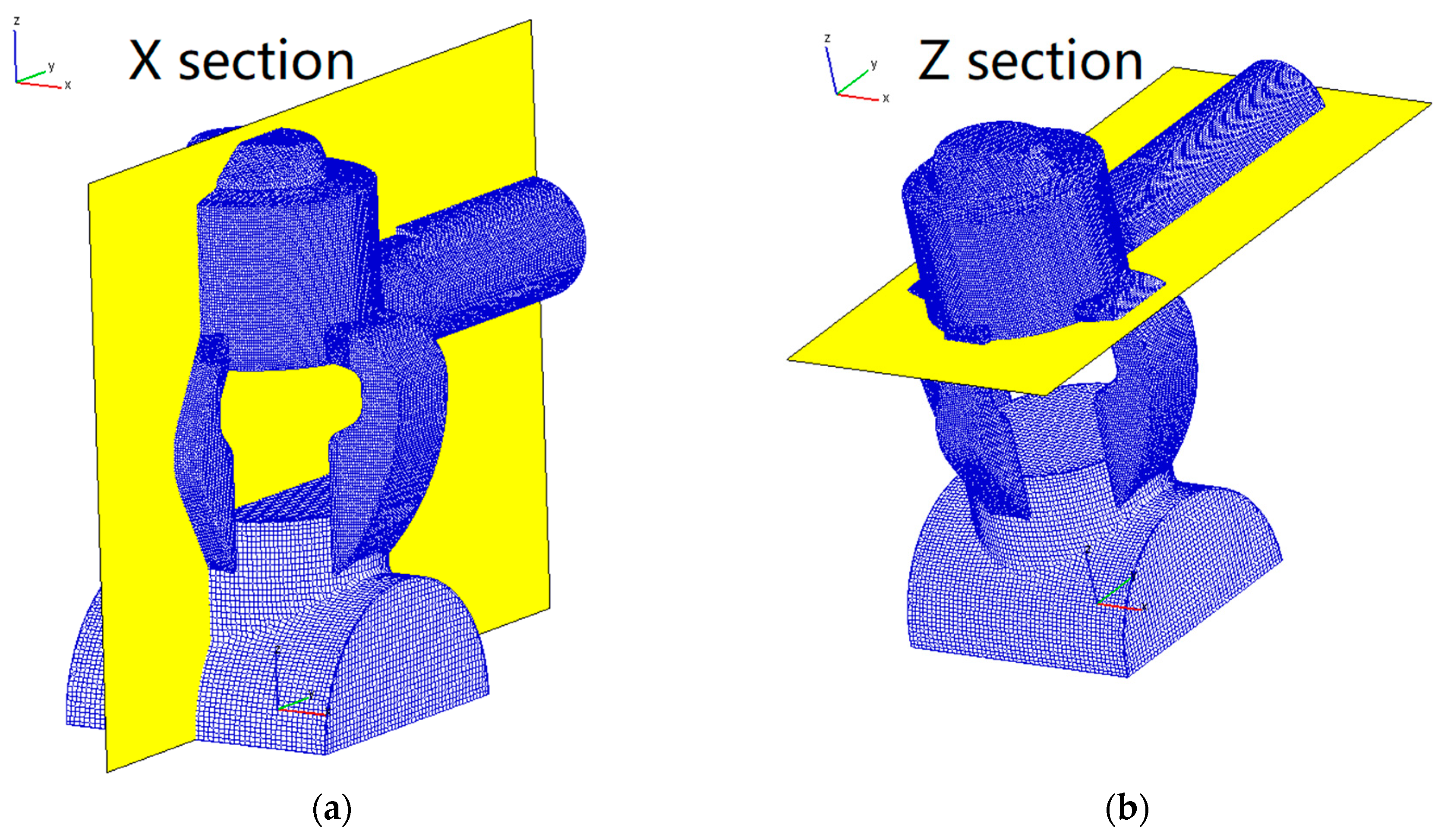
4.3. 3D Flow Field Visualization

With the powerful visualization tools provided by AVL FIRE simulation, various sectional views of the gas composition distribution inside the cylinder are accessible. As shown in Figure 18a, the X section passes through the cylinder axis and is exactly the symmetry plane of the cylinder. As shown in Figure 18b, the Z section is normal to the cylinder axis and passes through the center of four ports located on the cylinder wall.

150° CA, 180° CA, and 210° CA are selected as the representative crank angles of the whole scavenging process. X cross-sectional views and Z cross-sectional views of both the prototype engine and the optimal design under two different operating conditions are presented. The color in these figures indicates the proportion of fresh charge. The value of 1 indicates all fresh charge while 0 indicates all burned gas. The 3D flow field visualization results show that:

(1)

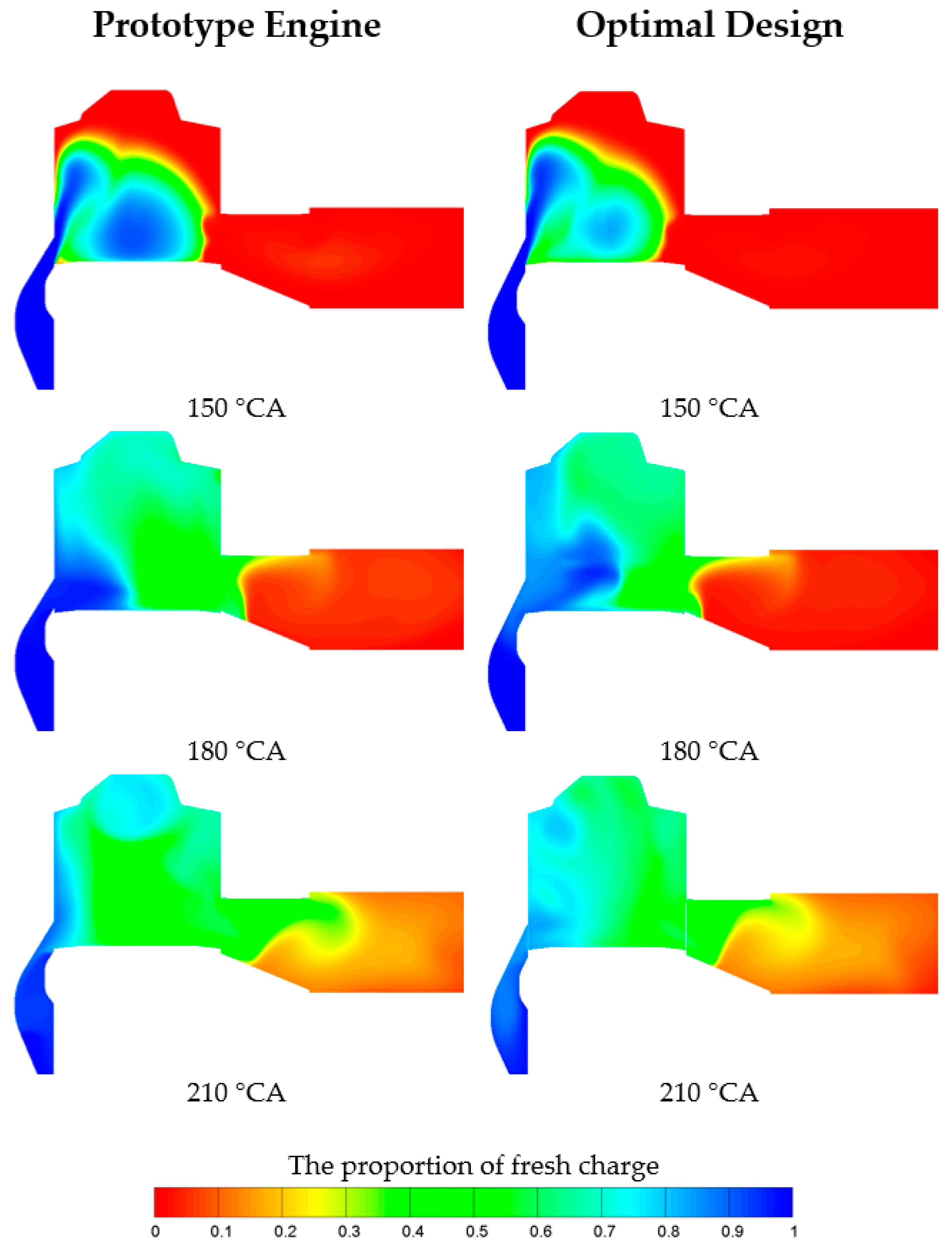
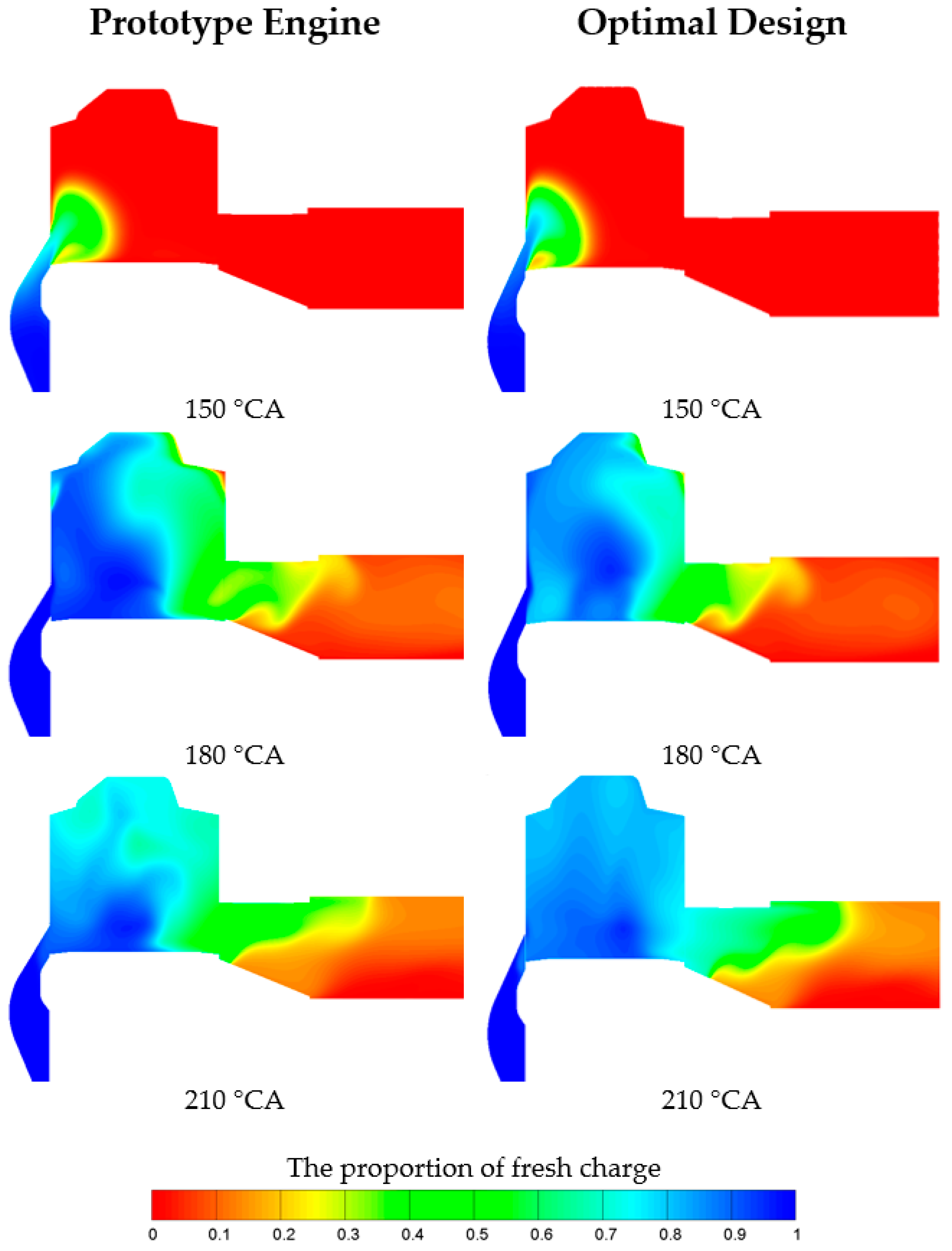
As shown in Figure 19, Figure 20, Figure 21 and Figure 22, when comparing the scavenging process of the prototype engine under two operating conditions, it is not difficult to find that the fresh intake charge under the high load is less than that of the partial load in the initial stage of the scavenging process (150 °CA). The in-cylinder pressure under the high load is higher than that of the partial load and the exhaust process takes a longer time, thus the in-cylinder pressure is still at a high level after the scavenging port opening. As a result, the pressure of the fresh charge is not enough to enter the cylinder in the early scavenging phase. Contrastingly, the fresh charge intake under the high load is notably more than that of the partial load at 180 °CA and 210 °CA. Because the throttle is wide open under the high load, the crankcase pressure is higher and the piston motion is faster and the crankcase scavenged process is more effective, thus more fresh charge is delivered into the cylinder. This significant difference can be perceived based on the ${\lambda }_S$ simulation data as well.

(2)

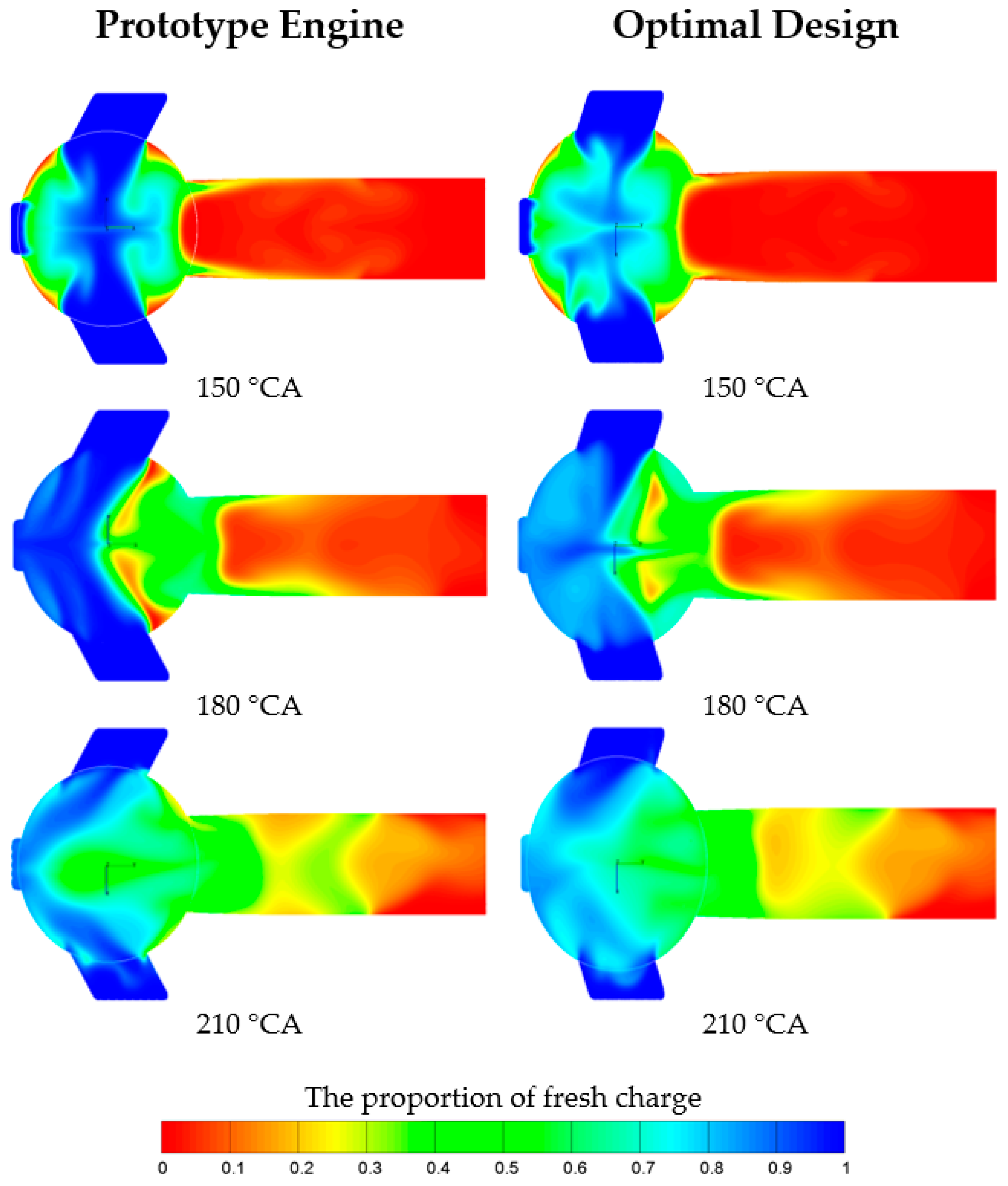
As shown in Figure 19 and Figure 20, when comparing the simulation results of the prototype engine and optimal design under the partial load, it can be found that at 150 °CA, the fresh charge intake of the prototype engine case is more than that of the optimal design case, especially around the lateral scavenging ports; at 180 °CA, the situation is similar to the high load simulation results, fresh charge distribution is biased toward the upper part of the cylinder with a larger “coverage area” after the optimal design; at 210 °CA, the optimal design results still show advantages over the prototype engine results in the scavenging quality. For the latter case, fresh charge is concentrated on the side of the central scavenging port as shown in the relevant Z cross-sectional views. Both lateral scavenging ports are inclined toward the central scavenging port. In consequence, corresponding gas motion due to the arrangement of the lateral scavenging ports hinders the fresh charge from entering the cylinder through the central scavenging port, and eventually gives rise to airflow obstruction and reduces the scavenging quality.

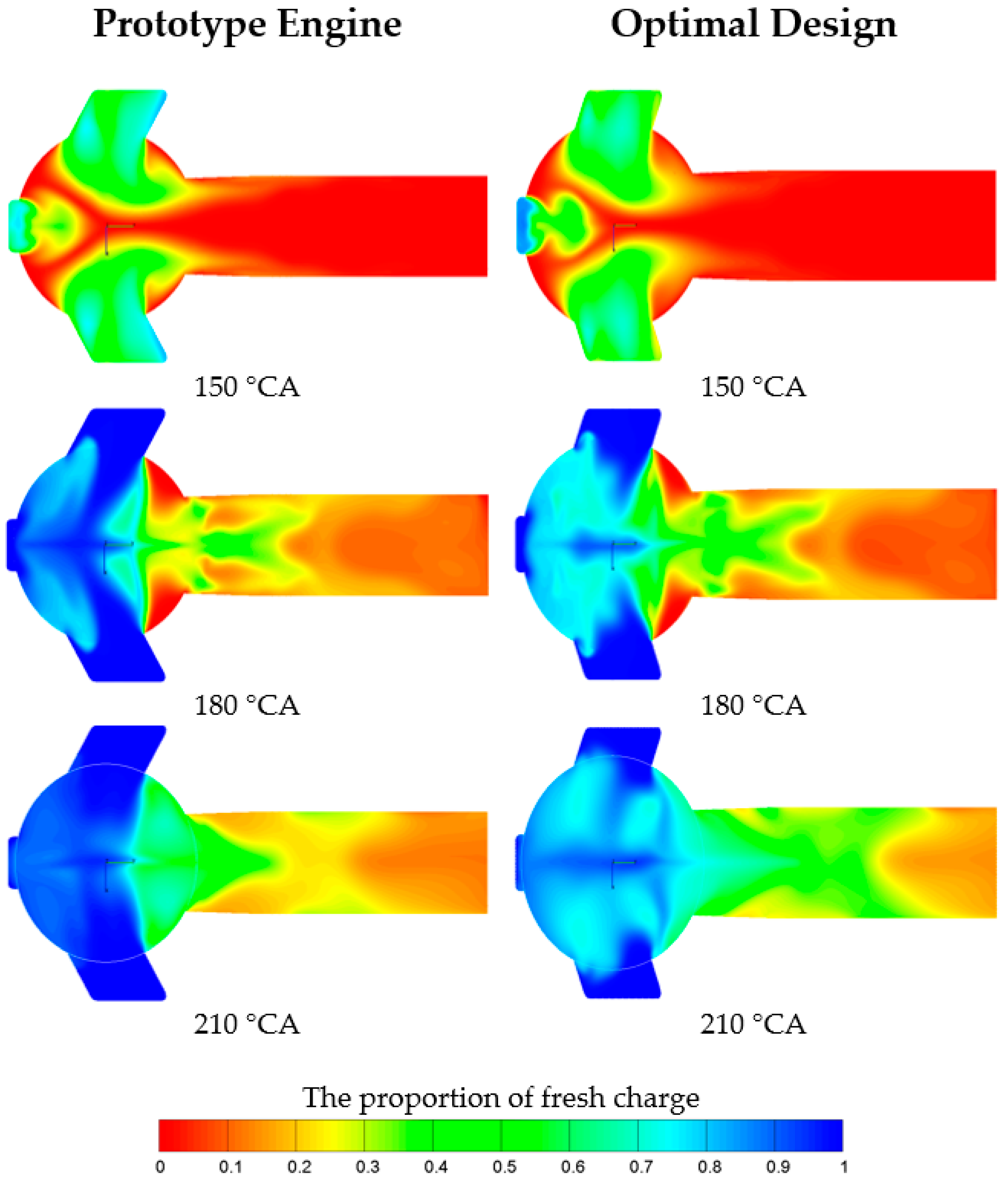
(3)

As shown in Figure 21 and Figure 22, when comparing the simulation results of the prototype engine and optimal design under the high load, it can be concluded that their gas composition distributions in the cylinder at 150 °CA are similar; at 180 °CA, fresh charge inside the cylinder is more biased toward the upper part in the optimal design results; at 210 °CA, fresh charge has reached more than 75% of the area of the entire cylinder after optimization. By contrast, the proportion of fresh charge in the combustion area is relatively low in the prototype engine case, which means the burned gas has not been cleared out of the cylinder even in the final scavenging phase.

Investigated factor values before and after optimization are displayed in

Table 10. Investigated factor values before and after optimization.

Factors	Prototype Engine	Optimal Design
${\alpha }_C$ (°)	55	60
${\alpha }_l$ (°)	0	20
${\beta }_l$ (°)	30	20
${\gamma }_C$	23.81%	23.81%

. Taken together, the optimal design has a larger ${\alpha }_C$ and ${\alpha }_l$, which yields better scavenging effects especially for the upper part of the cylinder, while a smaller ${\beta }_S$ alleviates the conflict impact resulted from the gas motion of fresh charge entering the cylinder through the central scavenging port and the lateral scavenging ports. The combination of these two points contributes to the optimal design results with a higher scavenging efficiency.

5. Discussion and Conclusions

As a common power source for widely applied small and medium-sized UAVs, the two-stroke small areoengine was selected as the research focus in this paper. Because of the particular scavenging system structure, the scavenging process features prominently in the engine power performance and fuel economy. Scavenging models are also proposed to describe the corresponding scavenging process. However, few previous researchers have paid enough attention to these more accurate and sophisticated scavenging models when optimizing the design of original ports’ arrangement. To illuminate this uncharted area, we selected the comprehensive evaluation objective function based on the Benson/Bradham model as the optimization goal and performed the 1D/3D coupling simulation to verify the optimal design results. Although demonstrated by preliminary simulation results, this optimization method suffers from some limitations due to the lack of a practical bench test of the redesigned two-stroke small areoengine. Despite that inadequacy, the present research findings provide the requisite criteria necessary for the appropriate design of a crankcase scavenging system, which plays a vital role in engine performance improvement. Detailed analysis leads to the following conclusions:

(1)

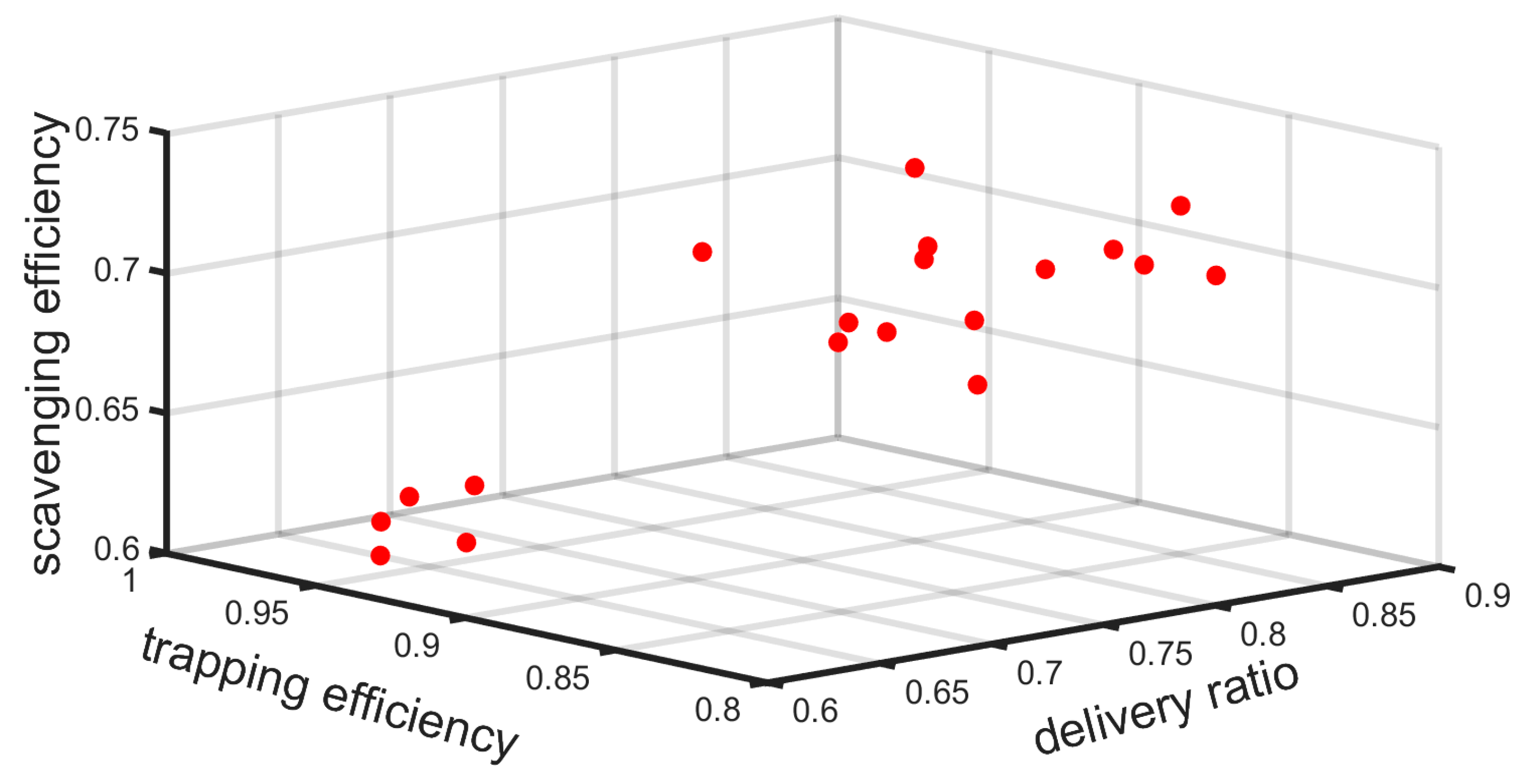
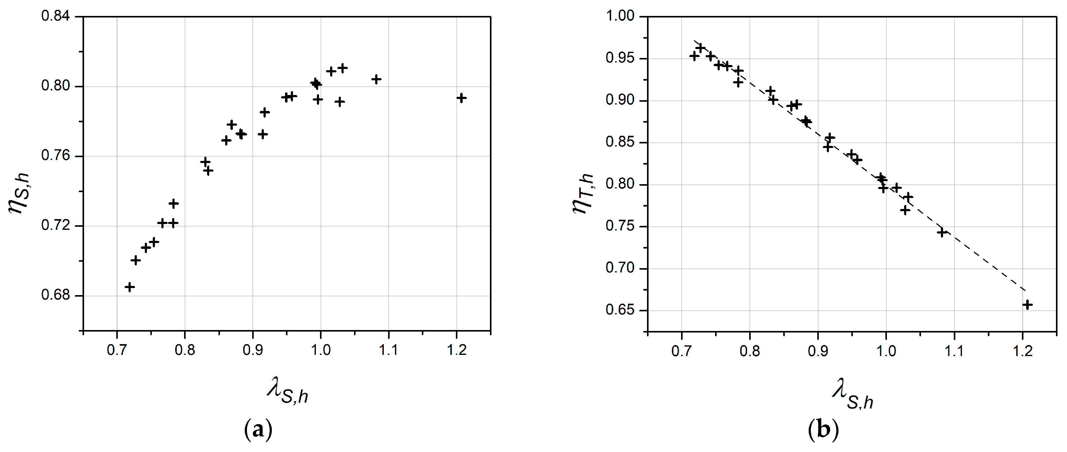
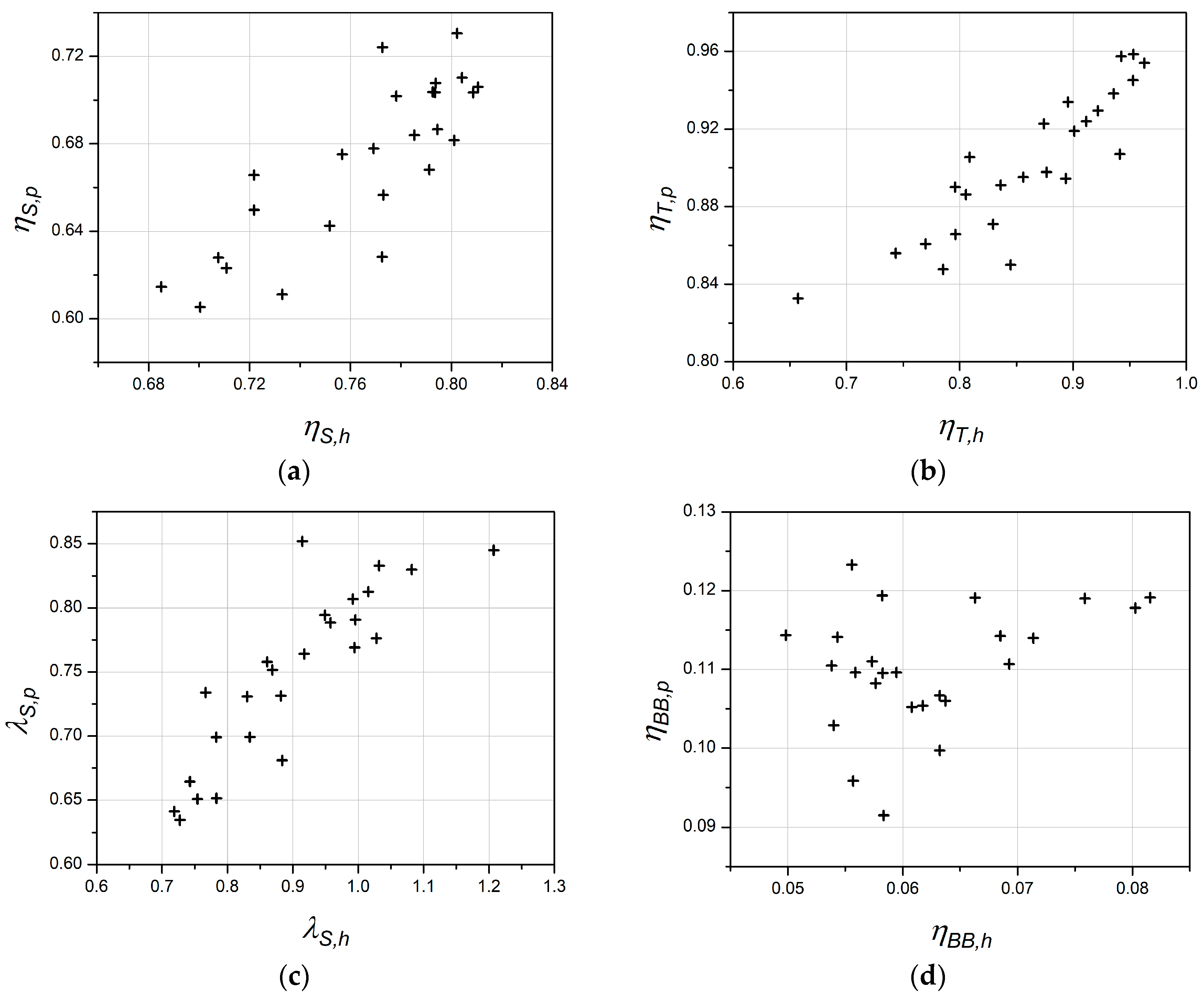
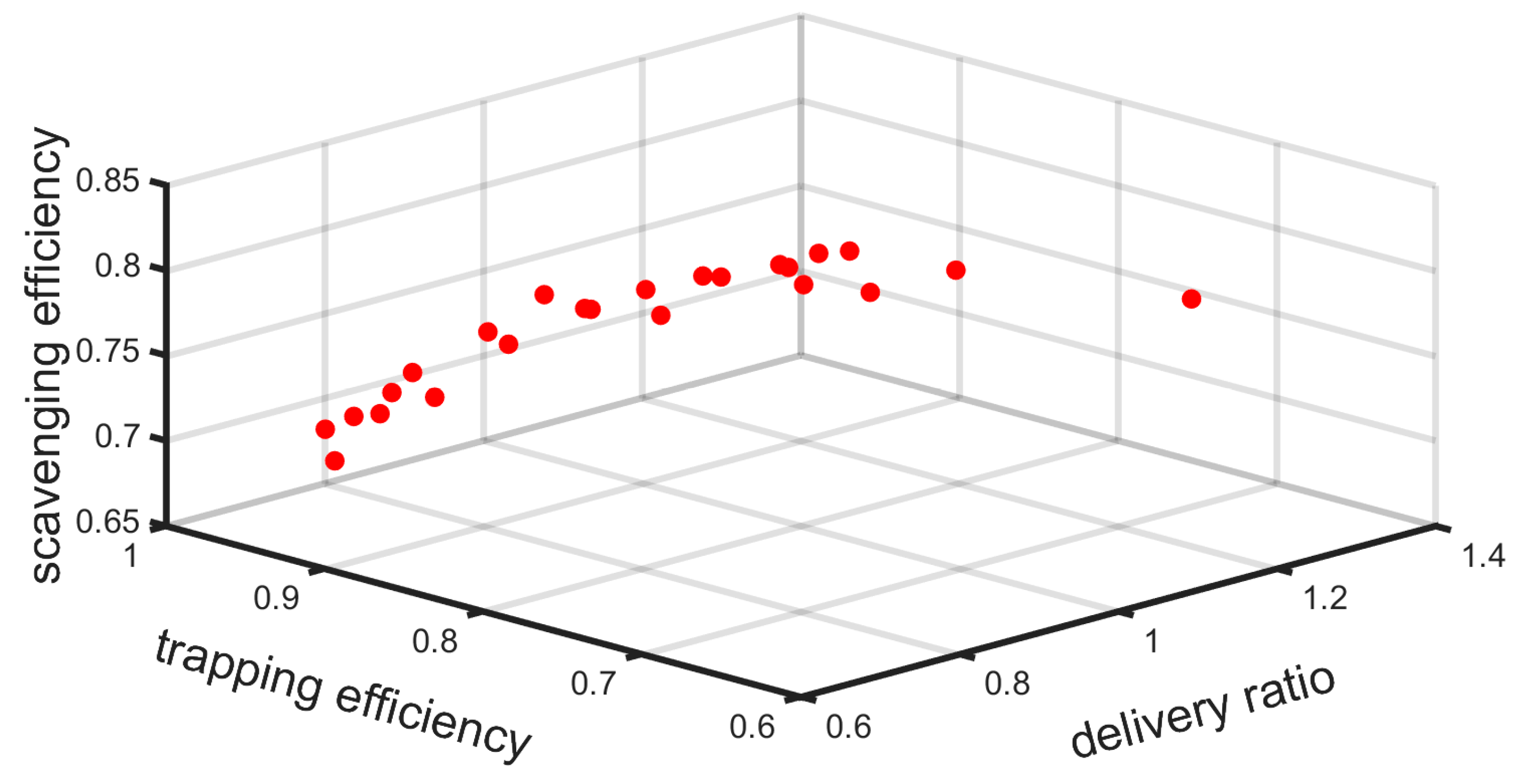
With respect to the investigated prototype engine scavenging system, there exists an obvious trade-off relationship between the scavenging efficiency, ${\eta }_S$, and trapping efficiency, ${\eta }_T$, which makes it difficult to balance the power performance and fuel economy during the optimization process.

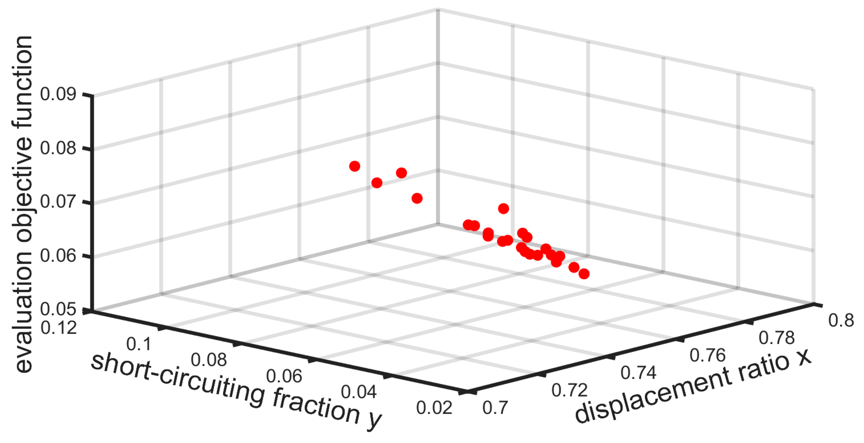
(2)

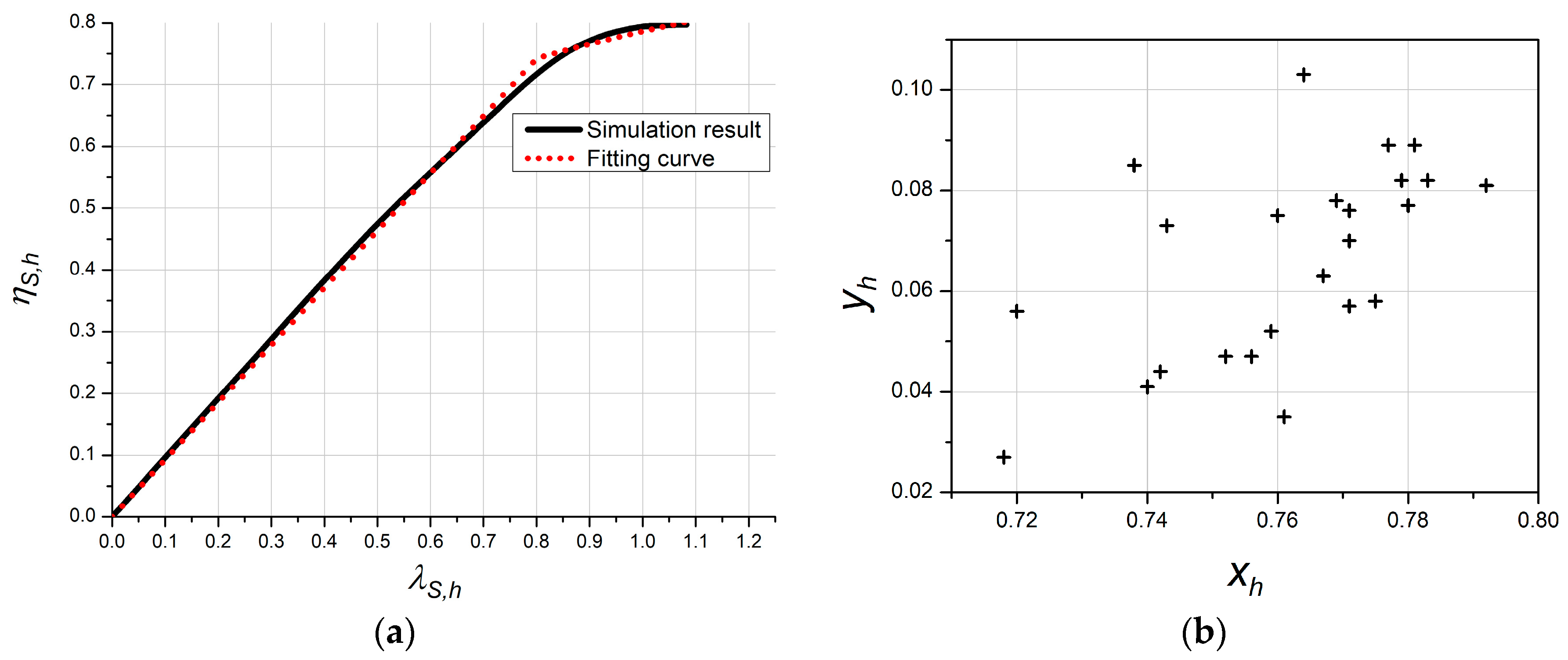
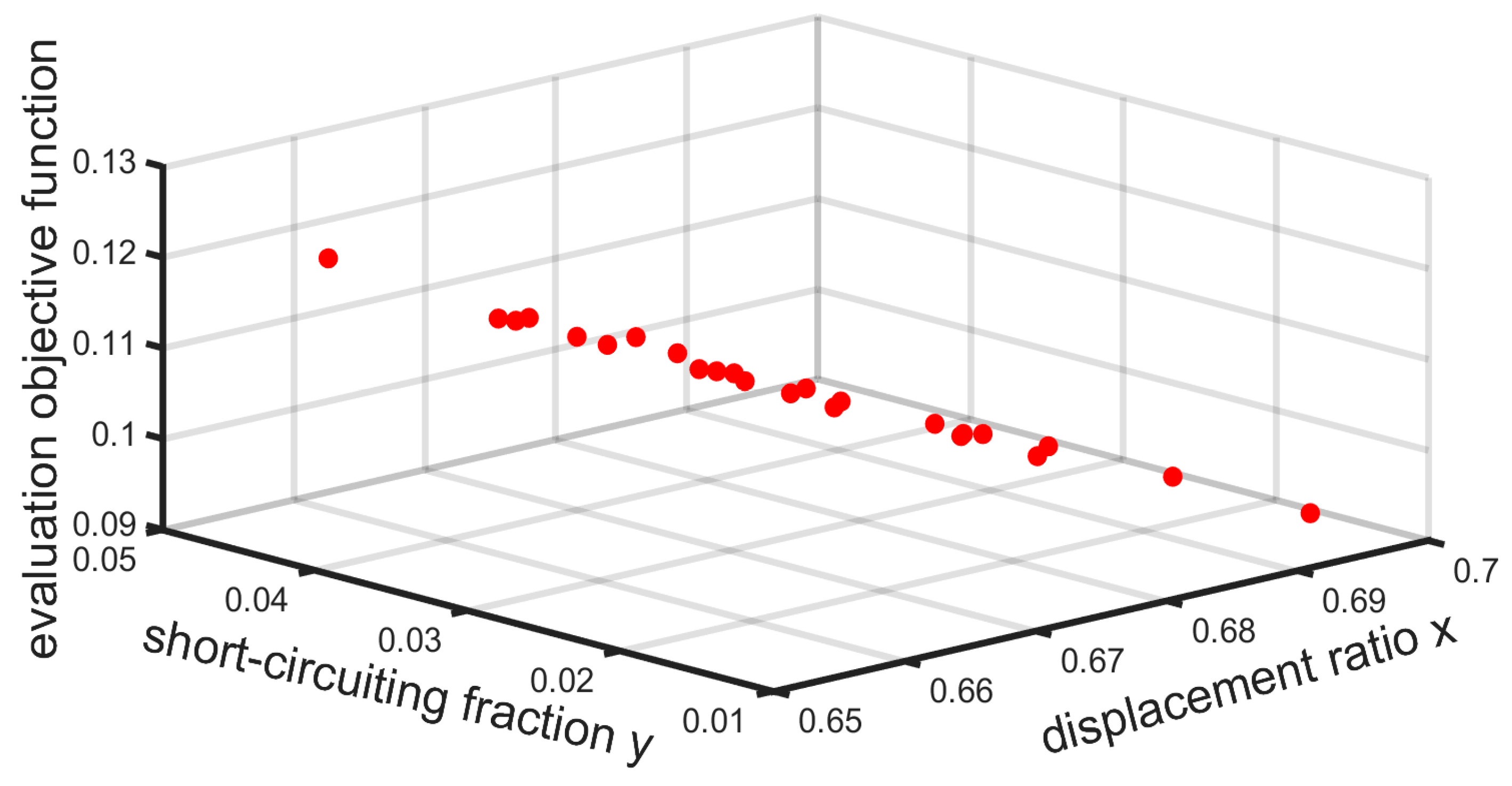
Characteristics of the actual gas exchange process can be indicated by the key parameters, $x$ and $y$, and the evaluation objective function, ${\eta }_{BB,c}$, based on the Benson/Bradham model was proven to reflect the scavenging quality precisely.

(3)

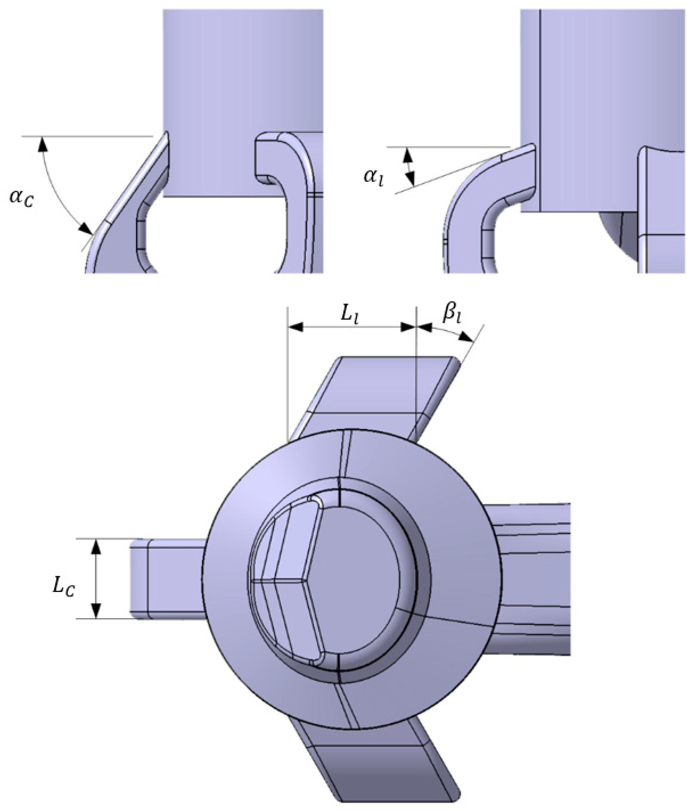
From the OED results analysis, it is clear that the slip angle of lateral scavenging ports, ${\beta }_l$, has the most significant influence on ${\eta }_{BB,c}$, followed by the tilt angle of lateral scavenging ports, ${\alpha }_l$, while the tilt angle of the central scavenging port, ${\alpha }_C$, and the width ratio of the central scavenging port, ${\gamma }_C$, are not statistically significant in terms of their influence on ${\eta }_{BB,c}$. The best factors combination is ${\alpha }_C$ = 60°, ${\alpha }_l$ = 20°, ${\beta }_l$ = 20°, and ${\gamma }_C$ = 23.81%.

(4)

Compared with the prototype engine, both ${\lambda }_S$ and ${\eta }_S$ in the optimal design results are improved, yet ${\eta }_T$ declines to some extent. Taken together, the optimal design results show superior progress in power performance (IMEP) while marginally deteriorations in the fuel economy (ISFC), which makes it still acceptable overall.

(5)

Powerful visualization tools provided by AVL FIRE software can be employed to analyze the gas composition distribution inside the cylinder during the whole scavenging process.

References

1. Ma, S.; Ma, L.; Xiao, B.; Yuan, Z. In Analysis of medium-sized unmanned aerial vehicle (UAV) maintenance and support organization. In Proceedings of the 2014 Prognostics and System Health Management Conference, Zhangjiajie, China, 24–27 August 2014; pp. 583–588. [Google Scholar]
2. Groff, E.G. Automotive Two-Stroke-Cycle Engine Development in the 1980–1990’s; Technical Paper for SAE International: Detroit, MI, USA, 2016. [Google Scholar]
3. Feng, G.; Zhou, M. Assessment of heavy fuel aircraft piston engine types. Tsinghua Sci. Technol. 2016, 56, 1114–1121. [Google Scholar]
4. Mavinahally, N.S. An Historical Overview of Stratified Scavenged Two-Stroke Engines-1901 through 2003; Technical Paper for SAE International: Detroit, MI, USA, 2004. [Google Scholar]
5. Hori, H. Scavenging Flow Optimization of Two-Stroke Diesel Engine by Use of CFD; Technical Paper for SAE International: Detroit, MI, USA, 2000. [Google Scholar]
6. Merker, G.P.; Gerstle, M. Evaluation on Two Stroke Engines Scavenging Models; Technical Paper for SAE International: Detroit, MI, USA, 1997. [Google Scholar]
7. Ma, F.; Zhao, Z.; Zhang, Y.; Wang, J.; Feng, Y.; Su, T.; Zhang, Y.; Liu, Y. Simulation Modeling Method and Experimental Investigation on the Uniflow Scavenging System of an Opposed-Piston Folded-Cranktrain Diesel Engine. Energies 2017, 10, 727. [Google Scholar] [CrossRef]
8. Brynych, P.; Macek, J.; Novella, R.; Thein, K. Representation of Two-Stroke Engine Scavenging in 1D Models Using 3D Simulations; Technical Paper for SAE International: Detroit, MI, USA, 2018. [Google Scholar]
9. Mattarelli, E.; Rinaldini, C.A.; Savioli, T. Port Design Criteria for 2-Stroke Loop Scavenged Engines; Technical Paper for SAE International: Detroit, MI, USA, 2016. [Google Scholar]
10. Wang, X.; Ma, J.; Zhao, H. Evaluations of Scavenge Port Designs for a Boosted Uniflow Scavenged Direct Injection Gasoline (BUSDIG) Engine by 3D CFD Simulations; Technical Paper for SAE International: Detroit, MI, USA, 2016. [Google Scholar]
11. Ma, J.; Zhao, H. The Modeling and Design of a Boosted Uniflow Scavenged Direct Injection Gasoline (BUSDIG) Engine; Technical Paper for SAE International: Detroit, MI, USA, 2015. [Google Scholar]
12. Wang, X.; Ma, J.; Zhao, H. Analysis of the Effect of Intake Plenum Design on the Scavenging Process in a 2-Stroke Boosted Uniflow Scavenged Direct Injection Gasoline (BUSDIG) Engine; Technical Paper for SAE International: Detroit, MI, USA, 2017. [Google Scholar]
13. Khoury, R.R.E.; Errera, M.; Khoury, K.E.; Nemer, M. Efficiency of coupling schemes for the treatment of steady state fluid-structure thermal interactions. Int. J. Therm. Sci. 2017, 115, 225–235. [Google Scholar] [CrossRef]
14. Rinaldini, C.A.; Mattarelli, E.; Golovitchev, V. CFD Analyses on 2-Stroke High Speed Diesel Engines. SAE Int. J. Engines 2011, 7, 2240–2256. [Google Scholar] [CrossRef]
15. Zirngibl, S.; Held, S.; Prager, M.; Wachtmeister, G. Experimental and Simulative Approaches for the Determination of Discharge Coefficients for Inlet and Exhaust Valves and Ports in Internal Combustion Engines; Technical Paper for SAE International: Detroit, MI, USA, 2017. [Google Scholar]
16. Nuccio, P.; Denno, D.D.; Magno, A. Development through Simulation of a Turbocharged 2-Stroke G.D.I. Engine Focused on a Range-Extender Application; Technical Paper for SAE International: Detroit, MI, USA, 2017. [Google Scholar]
17. Cui, L.; Wang, T.; Sun, K.; Lu, Z.; Che, Z.; Sun, Y. Numerical Analysis of the Steady-State Scavenging Flow Characteristics of a Two-Stroke Marine Engine; Technical Paper for SAE International: Detroit, MI, USA, 2017. [Google Scholar]
18. Xie, Z.; Zhao, Z.; Zhang, Z. Numerical Simulation of an Opposed-Piston Two-Stroke Diesel Engine; Technical Paper for SAE International: Detroit, MI, USA, 2015. [Google Scholar]
19. Zang, P.; Wang, Z.; Fu, Y.; Sun, C. Investigation of Scavenging Process for Steady-State Operation of a Linear Internal Combustion Engine-Linear Generator Integrated System; Technical Paper for SAE International: Detroit, MI, USA, 2017. [Google Scholar]
20. Mattarelli, E.; Rinaldini, C.A.; Savioli, T.; Cantore, G.; Warey, A.; Potter, M.; Gopalakrishnan, V.; Balestrino, S. Scavenge Ports Optimization of a 2-Stroke Opposed Piston Diesel Engine; Technical Paper for SAE International: Detroit, MI, USA, 2017. [Google Scholar]
21. Li, Z.; He, B.-q.; Zhao, H. Influences of intake ports and pent-roof structures on the flow characteristics of a poppet-valved two-stroke gasoline engine. Int. J. Engine Res. 2016, 17, 1077–1091. [Google Scholar] [CrossRef]
22. He, C.; Xu, S. Transient Gas Exchange Simulation and Uniflow Scavenging Analysis for a Unique Opposed Piston Diesel Engine; Technical Paper for SAE International: Detroit, MI, USA, 2016. [Google Scholar]
23. Zhou, L.; Zhang, H.; Zhao, Z.; Zhang, F. Research on Opposed Piston Two-Stroke Engine for Unmanned Aerial Vehicle by Thermodynamic Simulation; Technical Paper for SAE International: Detroit, MI, USA, 2017. [Google Scholar]
24. Zhao, F. Simulation Analysis and Optimization on the Scavenging Process for the Uniflow-Scavenge Diesel Engine. Master’s Thesis, Dalian University of Technology, Dalian, China, 6 July 2010. [Google Scholar]
25. Grljušić, M.; Tolj, I.; Radica, G.; Sciubba, E. An Investigation of the Composition of the Flow in and out of a Two-Stroke Diesel Engine and Air Consumption Ratio. Energies 2017, 10, 1. [Google Scholar] [CrossRef]
26. Taylor, C.F. The Internal-Combustion Engine in Theory and Practice: Thermodynamics, Fluid Flow, Performance, 2nd ed.; MIT Press: Cambridge, UK, 1985. [Google Scholar]
27. Γ Technologies, Engine Performance Application Manual, GT-Power Version 7.1. Available online: http://www.gtisoft.com/ (accessed on 19 July 2018).
28. Ma, F.K.; Wang, J.; Feng, Y.N.; Zhang, Y.G.; Su, T.X.; Zhang, Y.; Liu, Y.H. Parameter Optimization on the Uniflow Scavenging System of an OP2S-GDI Engine Based on Indicated Mean Effective Pressure (IMEP). Energies 2017, 10, 368. [Google Scholar] [CrossRef]
29. Dong, X.F.; Zhao, C.L.; Zhang, F.J.; Zhao, Z.F.; Xie, Z.Y. Experiment on the Scavenging Process of Opposed-Piston Two-Stroke Diesel Engine. Trans. CSICE 2015, 33, 362–369. [Google Scholar]
30. Sher, E.; Harari, R. A simple and realistic model for the scavenging process in a crankcase-scavenged two-stroke cycle engine. Proc. Inst. Mech. Eng. Part A J. Power Energy 1991, 205, 129–137. [Google Scholar] [CrossRef]
31. Wu, J. Similar design method used on the port size on the two-stroke diesel engine. Trans. Eng. Thermophys. 1981, 2, 145–153. [Google Scholar]
32. Dang, D.; Wallace, F.J. Some single zone scavenging models for two-stroke engines. Int. J. Mech. Sci. 1992, 34, 595–604. [Google Scholar] [CrossRef]
33. Kim, I.Y.; DeWeck, O.L. Adaptive weighted sum method for multi-objective optimization: A new method for Pareto front generation. Struct. Multidiscip. Optim. 2006, 31, 105–116. [Google Scholar] [CrossRef]
Figure 1. (a) Perfect mixing model; (b) perfect displacement model.
Energies 11 02739 g001
Figure 2. Phase/zone concept of the Benson/Bradham model: (a) Phase I; (b) Phase II.
Energies 11 02739 g002
Figure 3. Scavenging efficiency-delivery ratio relationship of the Benson/Bradham model.
Energies 11 02739 g003
Figure 4. GT Power simulation model architecture.
Energies 11 02739 g004
Figure 5. Comparison of in-cylinder pressure curves between the experiment and GT Power simulation. (a) High load operating condition; (b) partial load operating condition.
Energies 11 02739 g005
Figure 6. Comparison of the engine cylinder. (a) Reconstruction computer aided design (CAD) result; (b) actual part.
Energies 11 02739 g006
Figure 7. Scavenging system model. (a) CAD model; (b) CFD calculation model.
Energies 11 02739 g007
Figure 8. Comparison of in-cylinder pressure curves between the experiment and AVL FIRE simulation. (a) High load operating condition; (b) partial load operating condition.
Energies 11 02739 g008
Figure 9. Ports’ arrangement of the prototype engine scavenging system.
Energies 11 02739 g009
Figure 10. Definitions of important geometric parameters.
Energies 11 02739 g010
Figure 11. The high load results. (a) Scavenging efficiency; (b) trapping efficiency.
Energies 11 02739 g011
Figure 12. Comparison between the high load results and the partial load results. (a) Scavenging efficiency; (b) trapping efficiency; (c) delivery ratio; (d) evaluation objective function.
Energies 11 02739 g012
Figure 13. The high load results. (a) Comparison between the simulation result and the fitting curve; (b) scatterplot of coefficients, x h and y h .
Energies 11 02739 g013
Figure 14. 3D Pareto front results of the high load operating condition.
Energies 11 02739 g014
Figure 15. 3D Pareto front results of the partial load operating condition.
Energies 11 02739 g015
Figure 16. 3D Pareto front results of the high load operating condition.
Energies 11 02739 g016
Figure 17. 3D Pareto front results of the partial load operating condition.
Energies 11 02739 g017
Figure 18. (a) X section; (b) Z section.
Energies 11 02739 g018
Figure 19. X cross-sectional views of the prototype engine simulation case and optimal design simulation case under the partial load operating condition.
Energies 11 02739 g019
Figure 20. Z cross-sectional views of the prototype engine simulation case and optimal design simulation case under the partial load operating condition.
Energies 11 02739 g020
Figure 21. X cross-sectional views of the prototype engine simulation case and optimal design simulation case under the high load operating condition.
Energies 11 02739 g021
Figure 22. Z cross-sectional views of the prototype engine simulation case and optimal design simulation case under the high load operating condition.
Energies 11 02739 g022