Building Energy Management Strategy Using an HVAC System and Energy Storage System

Abstract

Recently, a worldwide movement to reduce greenhouse gas emissions has emerged, and includes efforts such as the Paris Agreement in 2015. To reduce greenhouse gas emissions, it is important to reduce unnecessary energy consumption or use environmentally-friendly energy sources and consumer products. Many studies have been performed on building energy management systems and energy storage systems (ESSs), which are aimed at efficient energy management. Herein, a heating, ventilation, and air-conditioning (HVAC) system peak load reduction algorithm and an ESS peak load reduction algorithm are proposed. First, an HVAC system accounts for the largest portion of building energy consumption. An HVAC system operates by considering the time-of-use price. However, because the indoor temperature is constantly changing with time, load shifting can be expected only immediately prior to use. Therefore, the primary objective is to reduce the operating time by changing the indoor temperature constraint at the forecasted peak time. Next, numerous research initiatives on ESSs are ongoing. In this study, we aim to systematically design the peak load reduction algorithm of ESS. The structure is designed such that the algorithm can be applied by distinguishing between the peak and non-peak days. Finally, the optimization scheduling simulation is performed. The result shows that the electricity price is minimized by peak load reduction and electricity usage reduction. The proposed algorithm is verified through MATLAB simulations.

1. Introduction

Over the past 40 years, the global consumption of primary energy has increased by approximately 2.4 times. Primary energy consumption has steadily increased, except for certain periods, such as the oil shock and financial crisis. Global energy demand is expected to continue to increase in the upcoming years. By 2040, the world energy demand is expected to increase by 30%. In response to the rapidly changing climate, the 21st Conference of the Parties to the United Nations Framework Convention on Climate Change was held in Paris at the end of 2015, with the aim of reducing greenhouse gas emissions. This move to control greenhouse gas emissions is occurring worldwide to raise the awareness about indiscriminate energy consumption. Hence, renewable energy generation such as solar power generation and wind power generation are spreading worldwide. However, the growth rate of new energy sources is limited and high investment costs are required. Therefore, technologies for efficiently using the existing energy are emerging. According to the data published by the U.S. Energy Information Administration in 2017, the heating, ventilation, and air-conditioning (HVAC) system is a heavy load, which accounts for approximately 25% of the total building load [1]. A typically used HVAC system operates to maintain the indoor temperature constant with the set temperature constant. Because of this feature, the HVAC system produces a constant output even at the peak load time, which is a burden to the user in terms of economy. In addition, on the grid side, HVAC systems can increase the required power plant capacity, generation and operating reserve capacity owing to increased peak loads. However, the HVAC system can control the set temperature; therefore, if it is controlled according to the electricity price and outdoor temperature by time, it has the potential to reduce the power consumption or peak load [2]. Another method to efficiently utilize the energy that is being used is via an energy storage system (ESS). The use of ESSs in buildings, which accounts for a significant portion of power consumption, is becoming a necessity for efficient demand management. Recently, the need for energy management has increased. HVAC system and ESS optimization scheduling has been studied extensively. Most of the studies using the HVAC system thus far have only considered reducing the load by modifying the indoor temperature constraint during the demand response time, and simulated by simplifying the thermal model. Thus, controlling the HVAC system only in the demand response time does not account for the economic benefits obtained from other times [3]. Further, a disadvantage is that the thermal model is simple and not similar to the actual temperature change pattern [4]. Significant work has been performed to manage the peak load using the ESS. Electricity costs can be divided into two categories: demand cost and energy cost. Strategies to minimize both the demand cost and energy cost are different. Previous studies have adopted necessary strategies, but the overall process was difficult to understand [5,6]. In the current work, we study the peak load reduction algorithm with the two systems above. Energy management using the HVAC system was designed considering the thermal model and user convenience, and the primary theme was to perform load shifting simultaneously with peak load reduction. The energy management algorithm using the ESS was used to design the structure, such that the overall process of minimizing the demand cost and energy cost can be organized by a single algorithm.

We herein introduce the uptime optimization scheduling of the HVAC system, and the output power optimization scheduling algorithm of the ESS for an optimal energy management. In the first of the two energy management strategies, the HVAC system schedules an uptime to reduce the day’s peak load. This does not simply stop the system at the peak time, but aims to maintain the proper indoor temperature considering user convenience. The change in the indoor temperature was implemented using the thermal model provided by MATLAB (R2017a, ‎The MathWorks Inc., Natick, MA, USA) to demonstrate a similar temperature change pattern. HVAC system optimization scheduling was performed by applying a genetic algorithm (GA). Next, the energy management algorithm using ESS is divided into two stages, and ESS output scheduling is implemented through the appropriate stage depending on the load at that time. ESS power optimization scheduling was performed by applying linear programming. Energy management simulations were performed using MATLAB.

Section 2 presents the algorithm for energy management using the HVAC system. Section 3 presents the algorithm for energy management using the ESS. The purpose of each stage and the formulae used are shown in detail. Section 4 shows the simulation results of the proposed algorithms using various cases. Finally, Section 5 presents the conclusions and the next steps of the presented study.

2. Energy Management Using HVAC System

2.1. Thermal Model and User Convenience in HVAC System

In HVAC systems, the indoor and outdoor temperatures are closely related to the load. The outdoor temperature is estimated at the meteorological office site, and it is important to model the indoor temperature with characteristics similar to those of actual HVAC systems [7]. In particular, the indoor temperature changes must be considered simultaneously with changes in HVAC system operation and outdoor temperature. In addition, the indoor temperature is affected by various factors, such as the structure of the building and the specifications of the HVAC system. To reflect these characteristics, the thermal model provided by MATLAB is applied to the HVAC system energy optimization algorithm.

The thermal model is constructed considering the characteristics of the building and the characteristics of the HVAC system, and various parameters can be changed according to the site. The thermal model provided by MATLAB is shown in Figure 1. The model consists of Simulink, and the initial model is a heating system. In this study, a Simulink model is constructed as a script to implement the HVAC system optimization algorithm, and a heating system model is constructed by partially modifying the cooling system model [8]. The formulae for the thermal model are as follows.

$$\frac{\mathrm{d}{\mathrm{Q}}_{\mathrm{c}\mathrm{o}\mathrm{o}\mathrm{l}}(\mathrm{t})}{\mathrm{d}\mathrm{t}}=({\mathrm{T}}_{\mathrm{i}\mathrm{n}}(\mathrm{t})-{\mathrm{T}}_{\mathrm{c}\mathrm{o}\mathrm{o}\mathrm{l}})\times ({\mathrm{t}}_{\mathrm{i}\mathrm{n}\mathrm{t}}\times 3600)\times {\mathrm{M}}_{\mathrm{d}\mathrm{o}\mathrm{t}}\times \mathrm{c}[\mathrm{J}/\mathrm{s}\mathrm{e}\mathrm{c}]$$

(1)

$$\frac{\mathrm{d}{\mathrm{Q}}_{\mathrm{h}\mathrm{e}\mathrm{a}\mathrm{t}}(\mathrm{t})}{\mathrm{d}\mathrm{t}}=({\mathrm{T}}_{\mathrm{h}\mathrm{e}\mathrm{a}\mathrm{t}}-{\mathrm{T}}_{\mathrm{i}\mathrm{n}}(\mathrm{t}))\times ({\mathrm{t}}_{\mathrm{i}\mathrm{n}\mathrm{t}}\times 3600)\times {\mathrm{M}}_{\mathrm{d}\mathrm{o}\mathrm{t}}\times \mathrm{c}[\mathrm{J}/\mathrm{s}\mathrm{e}\mathrm{c}]$$

(2)

$$\frac{\mathrm{d}{\mathrm{Q}}_{\mathrm{l}\mathrm{o}\mathrm{s}\mathrm{s}}(\mathrm{t})}{\mathrm{d}\mathrm{t}}=({\mathrm{T}}_{\mathrm{o}\mathrm{u}\mathrm{t}}(\mathrm{t})-{\mathrm{T}}_{\mathrm{i}\mathrm{n}}(\mathrm{t}))/{\mathrm{R}}_{\mathrm{e}\mathrm{q}}[\mathrm{J}/\mathrm{s}\mathrm{e}\mathrm{c}]$$

(3)

$${\mathrm{P}}_{\mathrm{c}\mathrm{o}\mathrm{o}\mathrm{l}}(\mathrm{t})=\frac{\mathrm{d}\mathrm{Q}\mathrm{c}\mathrm{o}\mathrm{o}\mathrm{l}(\mathrm{t})}{\mathrm{d}\mathrm{t}}/1000[\mathrm{k}\mathrm{W}]$$

(4)

$${\mathrm{P}}_{\mathrm{h}\mathrm{e}\mathrm{a}\mathrm{t}}(\mathrm{t})=\frac{\mathrm{d}\mathrm{Q}\mathrm{h}\mathrm{e}\mathrm{a}\mathrm{t}(\mathrm{t})}{\mathrm{d}\mathrm{t}}/1000[\mathrm{k}\mathrm{W}]$$

(5)

$$\frac{\mathrm{d}{\mathrm{T}}_{\mathrm{i}\mathrm{n}}(\mathrm{t})}{\mathrm{d}\mathrm{t}}=\{\begin{array}{l}\frac{1}{{\mathrm{M}}_{\mathrm{a}\mathrm{i}\mathrm{r}}\times \mathrm{c}}\times \left(\frac{\mathrm{d}{\mathrm{Q}}_{\mathrm{l}\mathrm{o}\mathrm{s}\mathrm{s}}(\mathrm{t})}{\mathrm{d}\mathrm{t}}-\frac{\mathrm{d}{\mathrm{Q}}_{\mathrm{c}\mathrm{o}\mathrm{o}\mathrm{l}}(\mathrm{t})}{\mathrm{d}\mathrm{t}}\right),\mathrm{w}\mathrm{h}\mathrm{e}\mathrm{n}\mathrm{c}\mathrm{o}\mathrm{o}\mathrm{l}\mathrm{i}\mathrm{n}\mathrm{g}\mathrm{s}\mathrm{y}\mathrm{s}\mathrm{t}\mathrm{e}\mathrm{m}\\ \frac{1}{{\mathrm{M}}_{\mathrm{a}\mathrm{i}\mathrm{r}}\times \mathrm{c}}\times \left(\frac{\mathrm{d}{\mathrm{Q}}_{\mathrm{l}\mathrm{o}\mathrm{s}\mathrm{s}}(\mathrm{t})}{\mathrm{d}\mathrm{t}}+\frac{\mathrm{d}{\mathrm{Q}}_{\mathrm{h}\mathrm{e}\mathrm{a}\mathrm{t}}(\mathrm{t})}{\mathrm{d}\mathrm{t}}\right),\mathrm{w}\mathrm{h}\mathrm{e}\mathrm{n}\mathrm{h}\mathrm{e}\mathrm{a}\mathrm{t}\mathrm{i}\mathrm{n}\mathrm{g}\mathrm{s}\mathrm{y}\mathrm{s}\mathrm{t}\mathrm{e}\mathrm{m}\end{array}$$

(6)

$${\mathrm{T}}_{\mathrm{i}\mathrm{n}}(\mathrm{t}+1)={\mathrm{T}}_{\mathrm{i}\mathrm{n}}(\mathrm{t})+{\mathrm{t}}_{\mathrm{i}\mathrm{n}\mathrm{t}}\times \frac{\mathrm{d}{\mathrm{T}}_{\mathrm{i}\mathrm{n}}(\mathrm{t})}{\mathrm{d}\mathrm{t}}$$

(7)

Equations (1) and (2) represent the HVAC system heat flow in the cooling and heating modes, respectively. Here, ${\mathrm{t}}_{\mathrm{i}\mathrm{n}\mathrm{t}}$ denotes the algorithm control period, and in the subsequent simulation, the time interval is set to 5 min and its value is 1/12 (h); ${\mathrm{T}}_{\mathrm{i}\mathrm{n}}$ denotes the indoor temperature by the control cycle; ${\mathrm{T}}_{\mathrm{c}\mathrm{o}\mathrm{o}\mathrm{l}}$, ${\mathrm{T}}_{\mathrm{h}\mathrm{e}\mathrm{a}\mathrm{t}}$ denote the cooling supply temperature, the heating supply temperature; ${\mathrm{M}}_{\mathrm{d}\mathrm{o}\mathrm{t}}$, $\mathrm{c}$ denote the HVAC system supply air mass and air heat capacity, respectively. Equation (3) shows the heat loss owing to the outdoor temperature and shows the effect on the indoor temperature change. Here, ${\mathrm{R}}_{\mathrm{e}\mathrm{q}}$ denotes the building equivalent heat resistance. Equations (4) and (5) show the output in the cooling and heating modes in kW, respectively. Equation (6) is the variation of the indoor temperature considering heat flow by the HVAC system and heat loss by the outdoor temperature. In Equation (7), the indoor temperature is updated according to the value from Equation (6) [9,10].

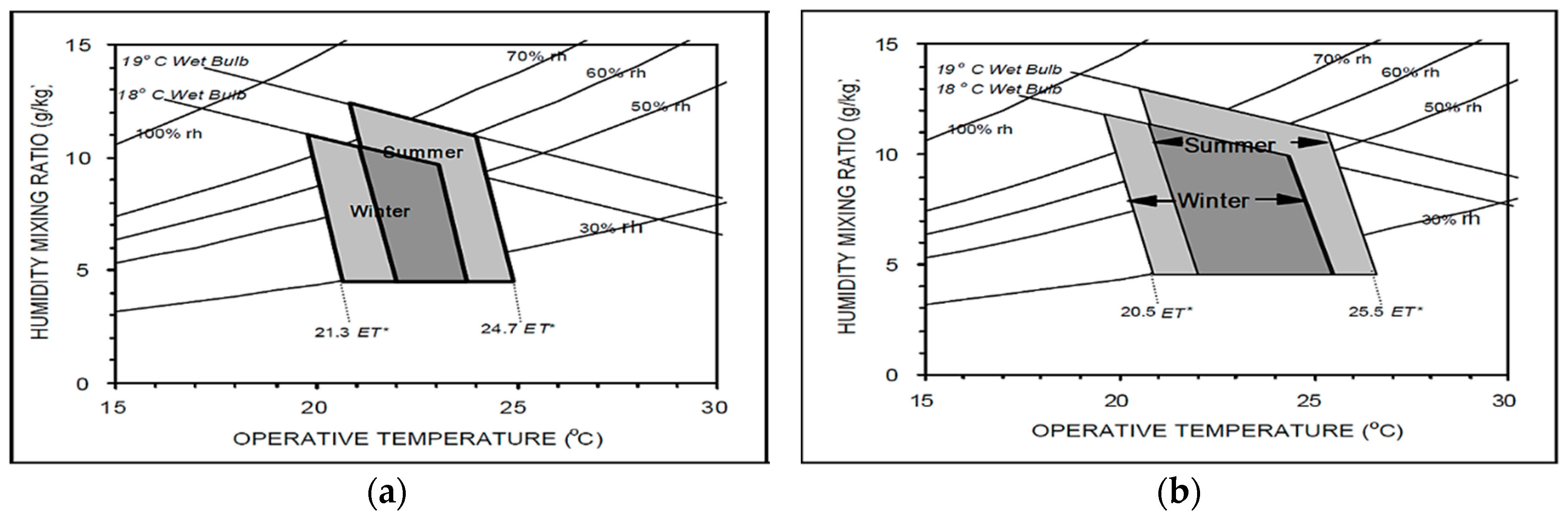
Once the optimal value is determined through the thermal model, the optimization scheduling of the HVAC system proceeds. The indoor temperature that the HVAC system must control is the most direct parameter that determines the user’s comfort. Hence, it is essential to consider user convenience in the energy optimization algorithm using the HVAC system. Figure 2 shows the range in which the user sees comfort in the psychrometric chart. The psychrometric chart shows the relationship among the dry bulb temperature, wet bulb temperature, absolute humidity, relative humidity, water vapor pressure, and enthalpy under atmospheric pressure [11,12]. The two graphs in Figure 2a,b demonstrate the range in which 90% and 80% of the users can feel comfortable, respectively. Because the 90% acceptability level is narrow, it is difficult to expect a load shifting effect to reduce the peak load at a specific time, or to reduce the energy cost through the HVAC operation. Meanwhile, the 80% acceptability level has a relatively wide tolerance range; therefore, the load peak or energy cost reduction can be expected through the proper operation of the HVAC. In the subsequent simulation, the relative humidity was set at 50% and the indoor temperature operating range is at the 80% acceptability level.

2.2. HVAC System Energy Management Optimization Algorithm

The objective function of the algorithm is to minimize the energy cost. The thermal model and user convenience described above are considered. The uptime of the HVAC system is regulated according to the electricity price. The HVAC system is operated at a time when the electricity price is low, thus reducing the operating number of HVAC systems at a relatively high electricity price. However, the pattern of the peak shifting is limited because the indoor temperature is continuously changed by the outdoor temperature. That is, even if the setting temperature is changed by operating at a specific time, it can only affect the next time. The objective function and the constraint conditions of the energy management optimization algorithm using the HVAC system are as follows.

$$\mathrm{M}\mathrm{i}\mathrm{n}\left\{{\displaystyle \sum _{\mathrm{t}=1}^{24/{\mathrm{t}}_{\mathrm{i}\mathrm{n}\mathrm{t}}}({\mathsf{\rho }}_{\mathrm{e}}(\mathrm{t})\times {\mathrm{t}}_{\mathrm{i}\mathrm{n}\mathrm{t}}\times \mathrm{u}(\mathrm{t})\times {\mathrm{P}}_{\mathrm{H}\mathrm{V}\mathrm{A}\mathrm{C}}(\mathrm{t}))}\right\}$$

(8)

$${\mathrm{P}}_{\mathrm{H}\mathrm{V}\mathrm{A}\mathrm{C}}(\mathrm{t})={\mathrm{u}}_{\mathrm{c}}(\mathrm{t})\times {\mathrm{P}}_{\mathrm{c}\mathrm{o}\mathrm{o}\mathrm{l}}(\mathrm{t})+{\mathrm{u}}_{\mathrm{h}}(\mathrm{t})\times {\mathrm{P}}_{\mathrm{h}\mathrm{e}\mathrm{a}\mathrm{t}}(\mathrm{t})$$

(9)

$$\mathrm{u}(\mathrm{t})={\mathrm{u}}_{\mathrm{c}}(\mathrm{t})+{\mathrm{u}}_{\mathrm{h}}(\mathrm{t})$$

(10)

$${\mathrm{u}}_{\mathrm{c}}(\mathrm{t})+{\mathrm{u}}_{\mathrm{h}}(\mathrm{t})\le 1$$

(11)

$${\mathrm{T}}_{\mathrm{i}\mathrm{n},\mathrm{m}\mathrm{i}\mathrm{n}}(\mathrm{t})\le {\mathrm{T}}_{\mathrm{i}\mathrm{n}}(\mathrm{t})\le {\mathrm{T}}_{\mathrm{i}\mathrm{n},\mathrm{m}\mathrm{a}\mathrm{x}}(\mathrm{t})$$

(12)

$${\mathrm{T}}_{\mathrm{w}\mathrm{o}\mathrm{r}\mathrm{k},\mathrm{m}\mathrm{i}\mathrm{n}}(\mathrm{t})\le {\mathrm{T}}_{\mathrm{i}\mathrm{n}}(\mathrm{t})\le {\mathrm{T}}_{\mathrm{w}\mathrm{o}\mathrm{r}\mathrm{k},\mathrm{m}\mathrm{a}\mathrm{x}}(\mathrm{t})$$

(13)

Equation (8) adjusts the operating time such that the energy cost is minimized as an objective function. Here, ${\mathsf{\rho }}_{\mathrm{e}}$, $\mathrm{u}$, ${\mathrm{P}}_{\mathrm{H}\mathrm{V}\mathrm{A}\mathrm{C}}$ denote the electricity price, the HVAC system on/off state, and the HVAC system power, respectively. Equations (9) and (10) represent the values of ${\mathrm{P}}_{\mathrm{H}\mathrm{V}\mathrm{A}\mathrm{C}}$ and $\mathrm{u}$ of the objective function, respectively; ${\mathrm{P}}_{\mathrm{c}\mathrm{o}\mathrm{o}\mathrm{l}}$ and ${\mathrm{P}}_{\mathrm{h}\mathrm{e}\mathrm{a}\mathrm{t}}$ are the cooling/heating power calculated in the thermal model; ${\mathrm{u}}_{\mathrm{c}}$ and ${\mathrm{u}}_{\mathrm{h}}$ are the binary variables indicating the cooling/heating state of the specific time, respectively. Equation (11) allows only one of the cooling and heating modes to operate at a specific time. Equation (12) represents the indoor temperature range constraint when the time is not the operating time or the peak load time, and this range can be changed according to the condition of the building. Equation (15) shows the indoor temperature range constraint considering user convenience at the operating time. The energy management algorithm of the HVAC system is optimized using the GA [13]. The optimal temperature range is set as a constraint condition considering user convenience, and the change in the indoor temperature is based on a thermal model [14,15]. Basically, it schedules the uptime according to the electricity price. If the peak load time of the day can be determined through the demand prediction, the peak load can be reduced by changing the indoor temperature range limit of the time [16,17].

3. Energy Management Using ESS

ESS can be used to reduce the electricity price and the peak load through charging and discharging. Thus, the cost of electric energy can be reduced. ESS can be more active in responding to peak control than the HVAC system load, and significant savings can be achieved if operated with proper output scheduling. The electricity costs are generally divided into the demand cost and energy cost. In this study, the process of minimizing the power consumption to determine the demand cost, as well as the power consumption to determine the energy cost are both structured systematically. 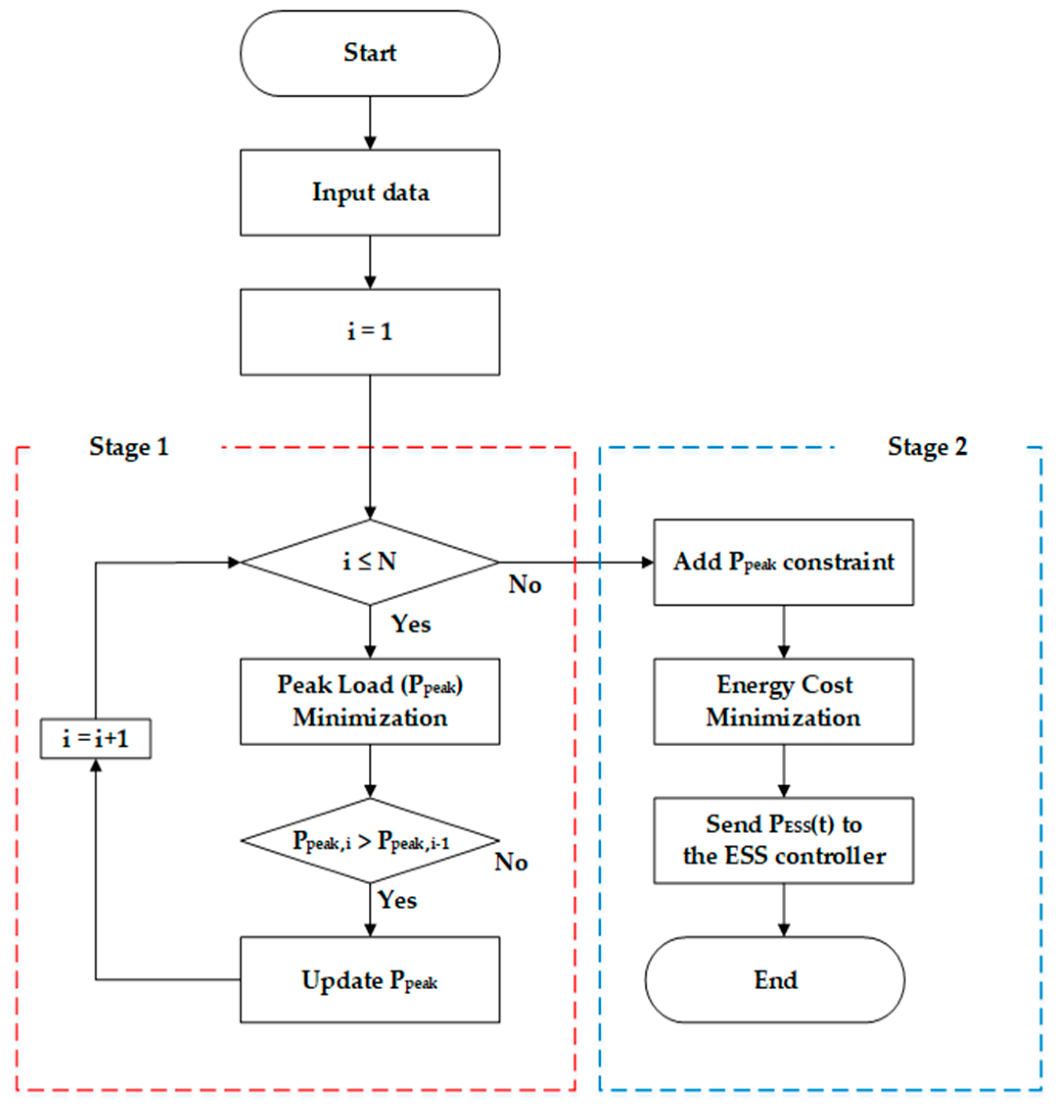Figure 3 shows the flow chart of the energy management optimization algorithm using the ESS. The algorithm is divided into Stage 1 and Stage 2. Stage 1 performs power scheduling to minimize the peak load. Stage 2 is developed to perform power scheduling to minimize the energy cost while not exceeding the peak load determined at Stage 1.

In Stage 1, peak load reduction scheduling using the ESS is performed using the predicted monthly load data. Simultaneously, the peak load (with ESS) is repeatedly compared to update the peak load that determines the monthly demand cost. The ESS output is determined according to the peak load reduction scheduling result when the peak load that determines the monthly demand cost is generated in the current month. In Stage 1, the objective function and constraint are as follows.

$$\mathrm{M}\mathrm{i}\mathrm{n}\{{\mathsf{\rho }}_{\mathrm{s}}\times {\mathrm{P}}_{\mathrm{p}\mathrm{e}\mathrm{a}\mathrm{k}}\}$$

(14)

$$-{\mathrm{P}}_{\mathrm{c}\mathrm{h},\mathrm{m}\mathrm{a}\mathrm{x}}\times \mathrm{x}(\mathrm{t})\le {\mathrm{P}}_{\mathrm{E}\mathrm{S}\mathrm{S}(\mathrm{t})}\le {\mathrm{P}}_{\mathrm{d}\mathrm{c}\mathrm{h},\mathrm{m}\mathrm{a}\mathrm{x}}\times \mathrm{y}(\mathrm{t})$$

(15)

$$\mathrm{x}(\mathrm{t})+\mathrm{y}(\mathrm{t})\le 1$$

(16)

$$\mathrm{S}\mathrm{O}\mathrm{C}(\mathrm{t})=\mathrm{S}\mathrm{O}\mathrm{C}(\mathrm{t}-1)-(\mathrm{y}(\mathrm{t})\times {\mathrm{P}}_{\mathrm{E}\mathrm{S}\mathrm{S}}(\mathrm{t})\times {\mathsf{\eta }}_{\mathrm{d}}{}^{-1}+\mathrm{x}(\mathrm{t})\times {\mathrm{P}}_{\mathrm{E}\mathrm{S}\mathrm{S}}(\mathrm{t})\times {\mathsf{\eta }}_{\mathrm{c}})$$

(17)

$$\mathrm{S}\mathrm{O}{\mathrm{C}}_{\mathrm{l}\mathrm{b}}\le \mathrm{S}\mathrm{O}\mathrm{C}\le \mathrm{S}\mathrm{O}{\mathrm{C}}_{\mathrm{u}\mathrm{b}}$$

(18)

$$\mathrm{S}\mathrm{O}{\mathrm{C}}_{\mathrm{f}\mathrm{i}\mathrm{n}\mathrm{a}\mathrm{l}}=\mathrm{S}\mathrm{O}{\mathrm{C}}_{\mathrm{i}\mathrm{n}\mathrm{i}\mathrm{t}\mathrm{i}\mathrm{a}\mathrm{l}}$$

(19)

$$\mathrm{L}\mathrm{o}\mathrm{a}\mathrm{d}(\mathrm{t})-{\mathrm{P}}_{\mathrm{E}\mathrm{S}\mathrm{S}}(\mathrm{t})\le {\mathrm{P}}_{\mathrm{p}\mathrm{e}\mathrm{a}\mathrm{k}}$$

(20)

Equation (14) is an objective function and consists of a base rate. ESS power scheduling is performed to lower the peak load. Here, ${\mathsf{\rho }}_{\mathrm{s}}$, ${\mathrm{P}}_{\mathrm{p}\mathrm{e}\mathrm{a}\mathrm{k}}$ denote the price per kW of the demand cost, i.e., the peak load. Equation (15) is a charging/discharging power constraint. The charging power has a negative value and the discharging power has a positive value. Here, ${\mathrm{P}}_{\mathrm{c}\mathrm{h},\mathrm{m}\mathrm{a}\mathrm{x}}$, ${\mathrm{P}}_{\mathrm{E}\mathrm{S}\mathrm{S}}$, ${\mathrm{P}}_{\mathrm{d}\mathrm{c}\mathrm{h},\mathrm{m}\mathrm{a}\mathrm{x}}$ denote the ESS charging rated power, the ESS power and the ESS discharging rated power, respectively. Equation (16) allows only one of the charging and discharging modes to operate at a specific time. Further, $\mathrm{x}$, $\mathrm{y}$ denote the ESS charging and discharging states, respectively. Both values are binary variables. Equation (17) is a formula for calculating the state of charge (SOC) for each control cycle. Here, ${\mathsf{\eta }}_{\mathrm{d}}$ and ${\mathsf{\eta }}_{\mathrm{c}}$ denote the ESS charging and discharging efficiencies, respectively. Equation (18) limits the operating range of the SOC of the ESS, and the final SOC is set equal to the initial SOC, as shown in Equation (19). Here, $\mathrm{S}\mathrm{O}{\mathrm{C}}_{\mathrm{l}\mathrm{b}}$ and $\mathrm{S}\mathrm{O}{\mathrm{C}}_{\mathrm{u}\mathrm{b}}$ denote the SOC lower and upper limits, respectively. Equation (20) shows that ${\mathrm{P}}_{\mathrm{p}\mathrm{e}\mathrm{a}\mathrm{k}}$ has the largest value among differences between the load and the ESS power.

When the peak load that determines the monthly demand cost is determined in Stage 1, Stage 2 adds the constraint using this value. In the objective function, the ESS performs power scheduling considering only the electricity price, excluding the demand cost portion. The objective function and the additional constraint condition in Stage 2 that minimizes the energy cost are as follows.

$$\mathrm{M}\mathrm{i}\mathrm{n}\left\{{\displaystyle \sum _{\mathrm{t}=1}^{96}({\mathsf{\rho }}_{\mathrm{e}}(\mathrm{t})\times 0.25\times (\mathrm{L}\mathrm{o}\mathrm{a}\mathrm{d}(\mathrm{t})}-{\mathrm{P}}_{\mathrm{E}\mathrm{S}\mathrm{S}}(\mathrm{t})))\right\}$$

(21)

$${\mathrm{P}}_{\mathrm{p}\mathrm{e}\mathrm{a}\mathrm{k}}\le {\mathrm{P}}_{\mathrm{p}\mathrm{e}\mathrm{a}\mathrm{k},\mathrm{l}\mathrm{i}\mathrm{m}\mathrm{i}\mathrm{t}}$$

(22)

According to Equation (21), the ESS performs optimization scheduling to charge at a low electricity price, and to discharge at a high electricity price considering the electricity price. Here, ${\mathsf{\rho }}_{\mathrm{e}}(\mathrm{t})$ denotes the electricity price. Equation (22) sets the peak load that determines the monthly demand cost as a constraint and limits the occurrence of new peak loads owing to the excessive charging of the ESS according to the electricity price. Here, ${\mathrm{P}}_{\mathrm{p}\mathrm{e}\mathrm{a}\mathrm{k},\mathrm{l}\mathrm{i}\mathrm{m}\mathrm{i}\mathrm{t}}$ means a peak load limit. The day when the peak load occurs in a month is preferentially scheduled in Stage 1 by the peak-reduction algorithm, and subsequently rescheduled to Stage 2.

4. Simulation Results

4.1. Simulation of HVAC System Optimization Algorithm

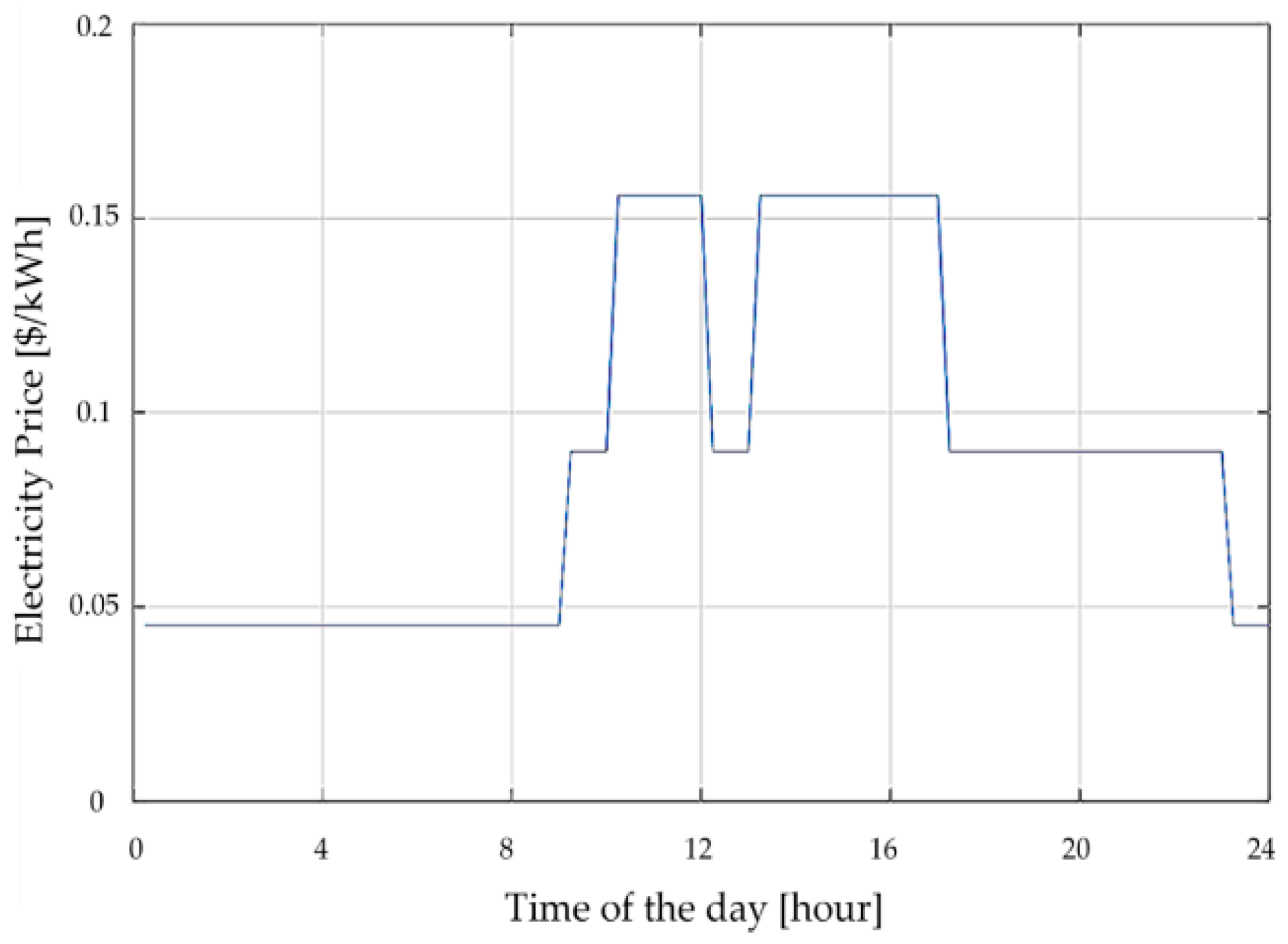
Our simulation is performed by modeling a real building and HVAC system using MATLAB. The building is modeled as a thermal model assuming a building size of 30 m × 10 m. The actual outdoor temperature is based on the actual data from 6 July 2015, in South Korea. The electricity cost is calculated using the actual hourly electricity price in Korea. The hourly electricity price is shown in Figure 4. First, it is assumed that the HVAC system does not operate, and the variation in the indoor temperature is confirmed when the indoor temperature changes only by the external temperature. A comparison of the indoor and outdoor temperatures is shown in Figure 5. The configuration data of the buildings are summarized in

Table 1. Configuration data of the building.

Parameter	Definition	Value	Parameter	Definition	Value
lenBuilding	Building Length	30 [m]	widWindows	Window Width	1 [m]
widBuilding	Building Width	10 [m]	htWindows	Window Height	1 [m]
htBuilding	Building Height	4 [m]	Req	Building Equivalent Heat Resistance	$1.73\times {10}^{-8}$ [sec∙°C/J]
numWindows	Number of Widows	6 [ea]	M	Indoor Air Mass	1470 [kg]

.

In this study, the simulation is performed for the summer. One day is composed of non-work time and work time, and the time from 2:00 p.m. to 3:00 p.m. is assumed to be the time when the peak load occurs. Scenarios for the HVAC system simulation are shown in

Table 2. Scenarios for the heating, ventilation, and air-conditioning (HVAC) system simulation.

Scenario	Setting Temperature (°C) (Non-Work Time/Work Time)	Indoor Temperature Range (°C) (Non-Work Time/Work Time)	Indoor Temperature Range at Peak Time (°C)
Case 1	27.5/23.5	−	−
Case 2	Scheduling	19.5~27.5/21.5~25.5	−
Case 3			19.5~27.5

.

4.1.1. Case 1

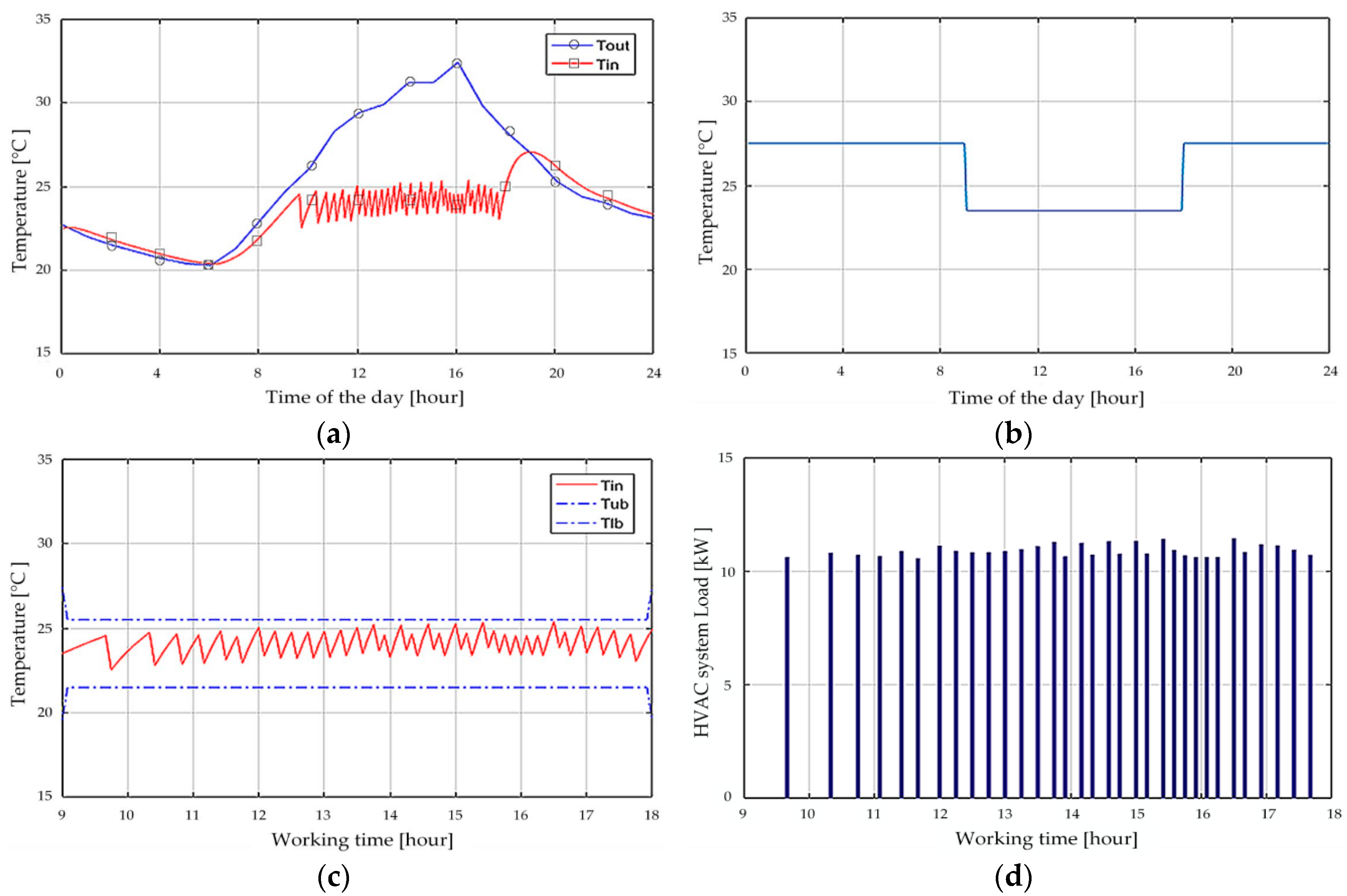
Case 1 is performed to observe the variation in the indoor temperature when the HVAC system is operated for the summer outdoor temperature change in the building model above. At this time, the HVAC system operates only when the set temperature and indoor temperature differ by 1 °C between 9:00 a.m. and 6:00 p.m., which is the work time. The control period is set to 5 min. The HVAC system data are summarized in

Table 3. Configuration data of the HVAC system.

Parameter	Definition	Value	Parameter	Definition	Value
Tcool	Cooling supply temperature	14 [°C]	Twork,max	Work time indoor temperature maximum	25.5 [°C]
Mdot	HVAC supply air mass	1 [kg/s]	Tin,min	Non-work time indoor temperature minimum	19.5 [°C]
Twork,min	Work time indoor temperature minimum	21.5 [°C]	Tin,max	Non-work time indoor temperature maximum	27.5 [°C]

.

We confirmed that the HVAC system is turned on/off as the daytime outdoor temperature increases. Therefore, the indoor temperature is maintained within a certain range. Case 1 is a general HVAC system because it operates at a constant temperature setting. The HVAC system output in Figure 6d is displayed every 5 min. Because the actual output is measured in units of 15 min, the unit load is obtained by averaging over a 15-min period. In the simulation, it is assumed that the peak of the total load occurs between 2:00 p.m. and 3:00 p.m. Therefore, the peak load of the HVAC system is as shown in

Table 4. Summary of Case 1 simulation results.

Scenario	Number of On/Off	Peak Load (2:00 p.m.~3:00 p.m.)	Power Consumption	Energy Cost
Case 1	33 [times]	7.36 [kW]	30.01 [kWh]	4.91 [$]

, summarizing the results, such as the number of on/off, power consumption, and energy cost.

4.1.2. Case 2

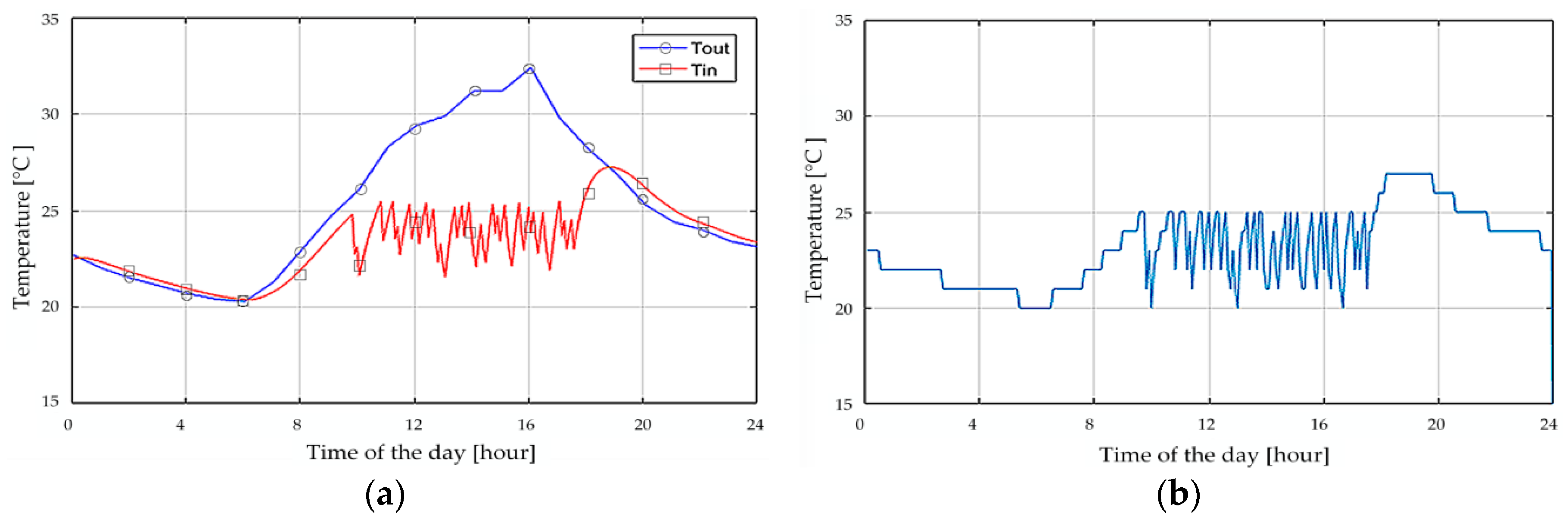
Case 2 uses the GA method to set the set temperature at which the energy cost is minimized. The simulation is performed using the same data as in Case 1 for the building data, HVAC system data, outdoor temperature data, and hourly electricity price data. Figure 7b shows the scheduled setting temperature. The HVAC system is turned on/off by comparing the setting temperature with the indoor temperature. To reduce the energy cost as much as possible, we confirmed that the cost is minimized by lowering the indoor temperature to as low as possible at 12:00 p.m. to 1:00 p.m., and increasing the indoor temperature at an expensive time. In Case 2, we confirmed that power consumption is increased compared to Case 1. This is because the difference between the indoor temperature of the current time and the outdoor temperature of the next time is increased as the indoor temperature is lowered as much as possible at a low electricity price. However, because the indoor temperature is changed according to the electricity price, the total energy cost is reduced by approximately $0.09 compared to Case 1.

Table 5. Summary of Case 2 simulation results.

Scenario	Number of On/Off	Peak Load (2:00 p.m.~3:00 p.m.)	Power Consumption	Energy Cost
Case 2	35 [times]	6.5 [kW]	30.43 [kWh]	4.82 [$]

summarizes the results of the number of on/off, peak load, power consumption, and energy cost.

4.1.3. Case 3

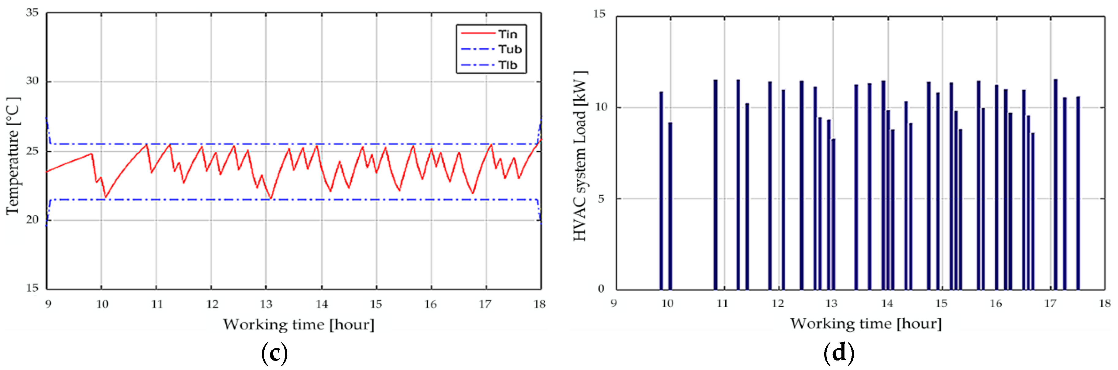
Case 3 controls the HVAC system at the setting temperature at which the energy cost is minimized using the GA method, as in Case 2. However, by maximizing the room temperature range from 2:00 p.m. to 3:00 p.m., which is assumed to be the peak load time, it is a simulation that reduces the peak load and minimizes the energy cost.

The data used is the same as those in Case 2, and the indoor temperature limit at 2:00 p.m. to 3:00 p.m. is changed as shown in

Table 6. Indoor temperature constraints between 2:00 p.m. and 3:00 p.m.

Parameter	Definition	Value	Parameter	Definition	Value
Twork,min	Work time indoor temperature minimum	19.5 [°C]	Twork,max	Work time indoor temperature maximum	27.5 [°C]

. In Case 3, the HVAC system also operates within a certain temperature range. Figure 8c shows the change in indoor temperature when the indoor temperature range from 2:00 p.m. to 3:00 p.m. is increased. In Case 3, the setting temperature is changed such that the energy cost is the lowest. In Case 3, the indoor temperature is increased to the maximum because the temperature range is increased from 2:00 p.m. to 3:00 p.m. Therefore, when cooling after 3:00 p.m., the HVAC peak load at every 5 min is higher than that of Case 2 to reduce the high temperature. Because the actual load is measured in units of 15 min, we confirmed that the peak load decreases from Case 2. In addition, because the setting temperature is maintained high when the electricity price is expensive, the energy cost is reduced by approximately $0.19 as compared to Case 2.

Table 7. Summary of Case 3 simulation results.

Scenario	Number of On/Off	Peak Load (2:00 p.m.~3:00 p.m.)	Power Consumption	Energy Cost
Case 3	32 [times]	4.52 [kW]	28.83 [kWh]	4.64 [$]

summarizes the results of the number of on/off, peak load, power consumption, and energy cost.

4.2. Simulation of ESS Optimization Algorithm

The ESS optimization algorithm is implemented and simulated using MATLAB. The actual load data from Inha University from February 2017 to August 2017 are used as the simulation load data. As a result of simulating all the dates by applying the algorithm of Stage 1, we confirmed that a peak load occurs on 7 August 2017. Hence, August 2017 is set as the simulation target. The rated power of the ESS is set to 2 MW, and the rated capacity to 2 MWh. The charging and discharging efficiencies are both set to 90%. The initial SOC and final SOC are both set at 50%, and the SOC operating range is set at 10 to 90%. The scenarios for the ESS simulation are shown in

Table 8. Scenarios for ESS simulation.

Scenario	ESS Configuration Data	Load Data	Characteristic
Case 1	2 MW/2 MWh Initial SOC: 50% Charging/Discharging efficiency: 90%	7 August 2017	Peak load (with ESS) Occurs
Case 2		9 August 2017	Peak load (without ESS) of Case 2 exceeds peak load (with ESS) of Case 1
Case 3		12 August 2017	Peak load (without ESS) of Case 3 less than peak load (with ESS) of Case 1

. The reason for configuring the scenario as shown below is that it can demonstrate all the situations that can occur.

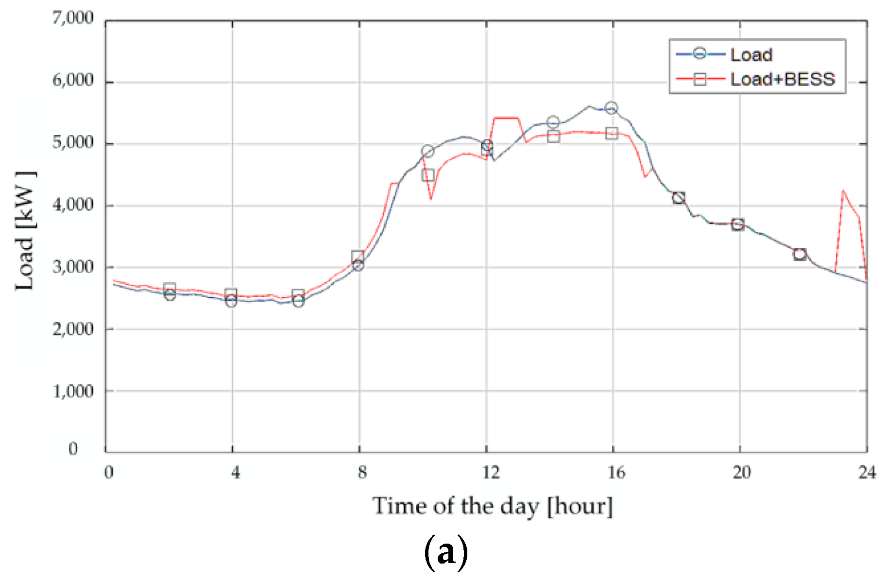
4.2.1. Case 1

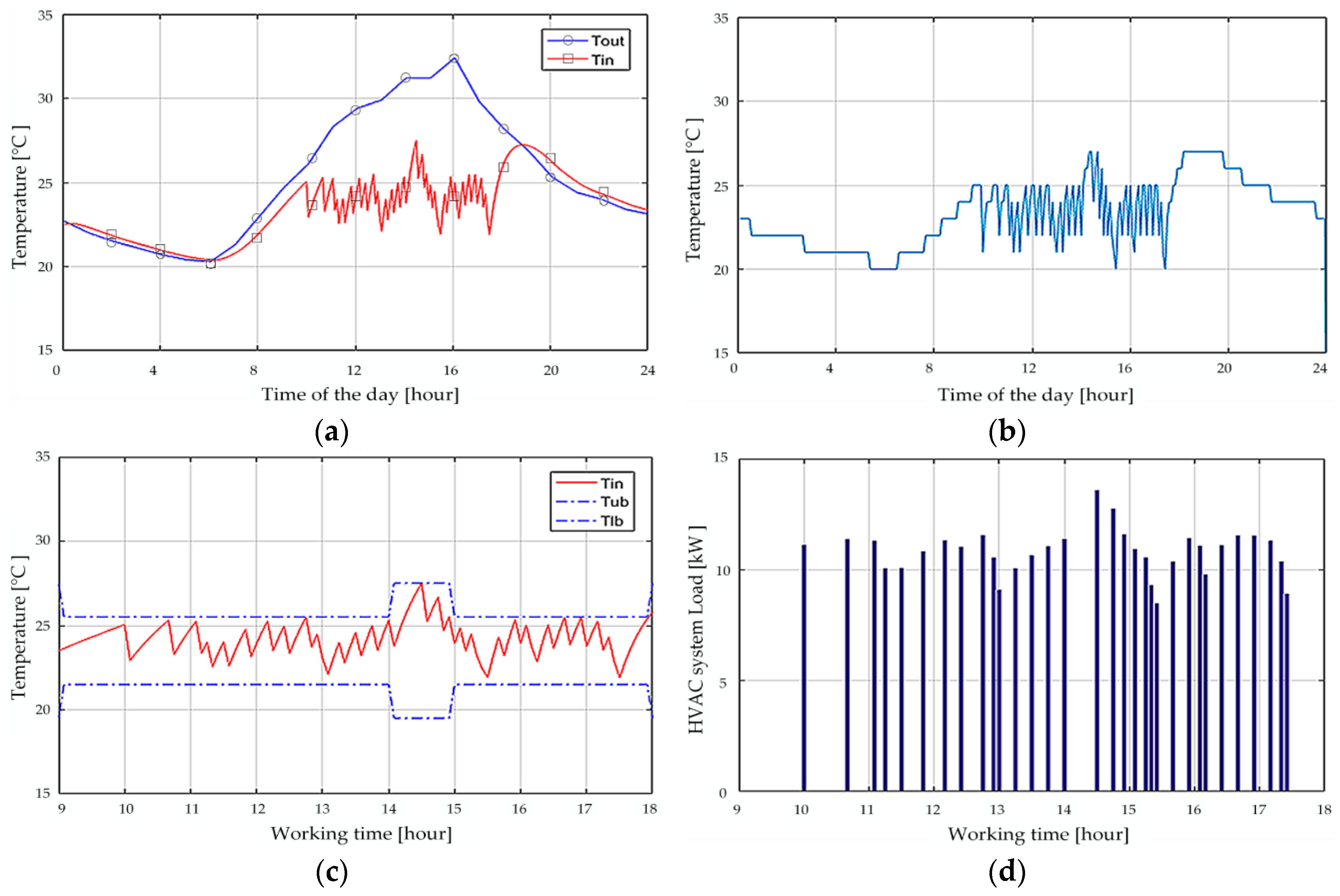
In Case 1, 7 August 2017 is the day when the peak load (including ESS) occurs. Hence, Stage 1 scheduling is performed to minimize the peak load (with ESS). Because the peak load reduction is the primary goal, the SOC is set to the maximum value before the peak time, and the discharging is continued from 1:00 p.m. to 5:00 p.m. Figure 9a shows that 479.4 kW is reduced at the original peak load using the ESS. Because the pattern of the original load is flat at the peak, the peak load reduction is not large. The results of Case 1 are summarized in

Table 9. Summary of Case 1 simulation results.

Scenario	Original Peak Load	New Peak Load (with ESS)	Demand Cost Reduction	Daily Energy Cost Reduction
Case 1	5900.2 [kW]	5420.8 [kW]	3097.9 [$]	136.8 [$]

, and the peak load that determines the demand cost in August is set at 5420.8 kW.

4.2.2. Case 2

Case 2 uses the load data of 9 August 2017. Stage 1 is assessed as not the peak load that determines the demand cost through the scheduling of minimizing the peak load; therefore, it goes to Stage 2 of the flowchart. The purpose of the simulation in Case 2 is to confirm the power scheduling of the ESS when the peak load exceeds the peak load that determines the demand cost. In Figure 10, because the demand cost is not included in the objective function, discharging is performed at a time when the electricity price is high to minimize the energy cost. Therefore, the ESS is charged at 12:00–1:00 p.m., owing to the low electricity price. However, it is not possible to increase the SOC to the maximum owing to the constraint of the peak load that determines the demand cost in Case 1. The simulation results demonstrate that the ESS charges from 11:00 p.m. to 12:00 a.m. to set the final SOC to the same value as the initial SOC. Because the simulation is performed only for one day, the ESS is charged from 11:00 p.m. to 12:00 p.m., and the lowest price is shown in the evening. The results of Case 2 are summarized in

Table 10. Summary of Case 2 simulation results.

Scenario	Original Peak Load	New Peak Load (with ESS)	Daily Energy Cost Reduction
Case 2	5614.1 [kW]	5420.8 [kW]	150.9 [$]

.

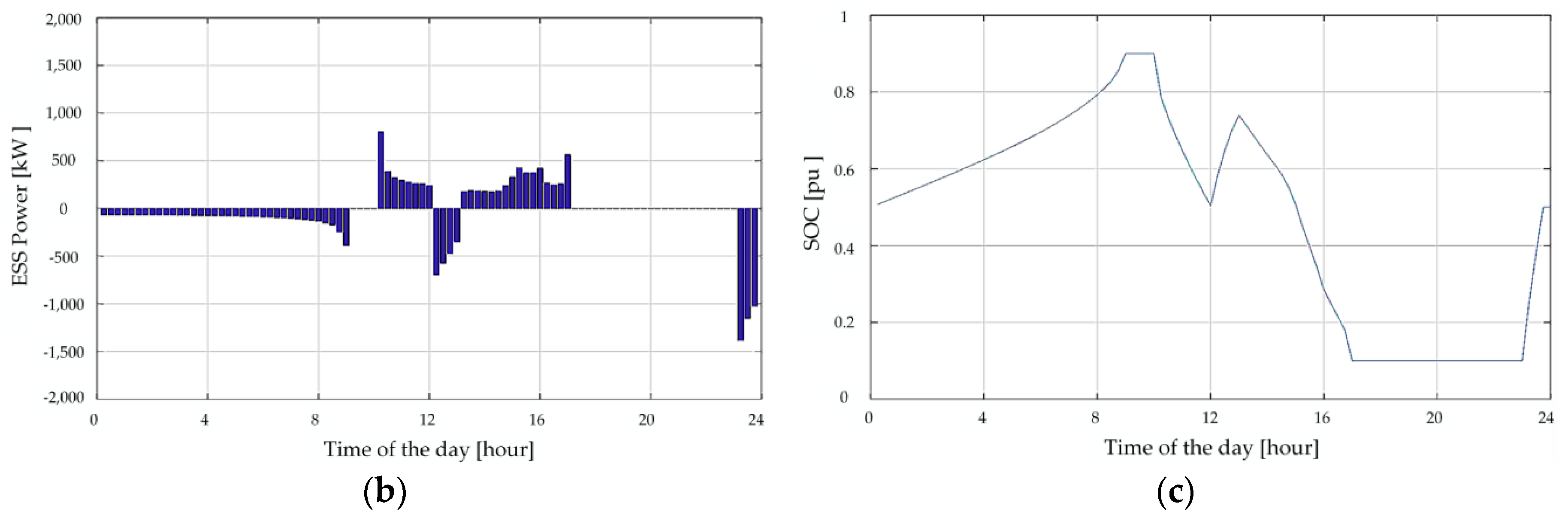
4.2.3. Case 3

In Case 3, the load data of 12 August 2017 are used. The peak is not high because Case 3 is a weekend load. The purpose simulating Case 3 is to confirm the power scheduling of the ESS when the peak load does not exceed the peak load that determines the demand cost. In Figure 11b,c, the ESS output power and SOC are similar to the patterns in Case 2. However, because the original peak load is low, the energy cost is minimized without violating the constraints. The peak load is increased by 539.7 kW when operating the ESS compared to the original peak load; however, it does not affect the demand cost. The results of Case 3 are summarized in

Table 11. Summary of Case 3 simulation results.

Scenario	Original Peak Load	New Peak Load (with ESS)	Daily Energy Cost Reduction
Case 3	3246.7 [kW]	4929.6 [kW]	193.1 [$]

.

5. Conclusions

We herein proposed a method to reduce the peak load by adjusting the operation time of the HVAC system at the peak load time. Algorithms were designed to receive the peak load time period and the electricity price as the input data; thus, the HVAC system performed uptime scheduling to minimize the peak load and energy cost. The thermal model provided by MATLAB was applied, and user convenience was considered. Through simulations, the operation of the algorithm was verified and the simulation results were analyzed. By operating the cooling in advance at a time when the electricity price was low, the indoor temperature was maintained within an appropriate range and the power consumption was reduced. In addition, by changing the room temperature limit during peak hours, we confirmed that the HVAC operation time and the peak of the entire load was reduced. In another energy management strategy, the ESS optimization algorithm was designed to schedule the outputs of the ESS systematically. This algorithm was divided into Stage 1 to reduce the peak load corresponding to the demand cost, and Stage 2 to minimize the overall energy cost. We confirmed that the scheduling was performed by distinguishing the stages through three simulations. The proposed algorithms demonstrated energy management strategies in a single building. The contribution of this paper is that different types of technologies can be controlled for the same purpose, peak load reduction and the energy cost saving. The HVAC system does not simply turn off at peak hours, but it can save the electricity cost while meeting user comfort. The ESS can reduce both the energy cost and the peak load by charging energy at the low price time and discharging at the high price time.

As future work, we will further study the design of an integrated aggregator for the participation of the electricity providers and consumers in many buildings applying the proposed algorithms.