PLDAD—An Algorihm to Reduce Data Center Energy Consumption

Abstract

Due to the demands of new technologies such as social networks, e-commerce and cloud computing, more energy is being consumed in order to store all the produced data. While these new technologies require high levels of availability, a reduction in the cost and environmental impact is also expected. The present paper proposes a power balancing algorithm (power load distribution algorithm-depth (PLDA-D)) to optimize the energy distribution of data center electrical infrastructures. The PLDA-D is based on the Bellman and Ford–Fulkerson flow algorithms that analyze energy-flow models (EFM). EFM computes the power efficiency, sustainability and cost metrics of data center infrastructures. To demonstrate the applicability of the proposed strategy, we present a case study that analyzes four power infrastructures. The results obtained show about a 3.8% reduction in sustainability impact and operational costs.

1. Introduction

Social awareness has influenced the way the world works and how people live. Widely available Internet access, the growing mobile market and advances in cloud computing technology are generating a huge amount of data, thus entailing unprecedented demands on energy consumption. The digital universe corresponds to 500 billion gigabytes of data [1], for which only 25% of the world’s population is on-line [2].

Data center power consumption has increased significantly over recent years, influenced by the increasing demand for storage capacity and data processing [3,4,5]. In 2013, data centers in the U.S. consumed 91 billion kilowatt-hours of electricity [6], and this is expected to continue to rise. In addition, critical elements in the performance of daily tasks, such as social networks, e-commerce and data storage, also contribute to the rise in energy consumption across these systems.

Data center infrastructures require electrical components, many of which may directly affect system availability. Fault-tolerant mechanisms are key techniques for handling equipment with limited reliability. The Uptime Institute [7] is an institution that classifies the infrastructure of the data center based on the architectures and characteristics of redundancy and fault tolerance (Tier I, Tier II, Tier III and Tier IV). In this paper, four data centers were analyzed, considering different tiers of architectures for the power subsystem. The power subsystem electrical flow is represented by the energy flow model (EFM) [8].

The algorithm proposed in this paper, named power load distribution algorithm-depth (PLDA-D), improves the results presented in our previous work when considering the operational cost and energy efficiency of data centers [8,9,10]. Now, we have obtained the shortest path, using Bellman algorithm instructions, considering the energy cost as the main metric and the maximum energy flow (Ford–Fulkerson), considering the energy efficiency of each component of the data center’s electrical infrastructure. Thus, we propose this new algorithm that uses two criteria of different classes that complement each other.

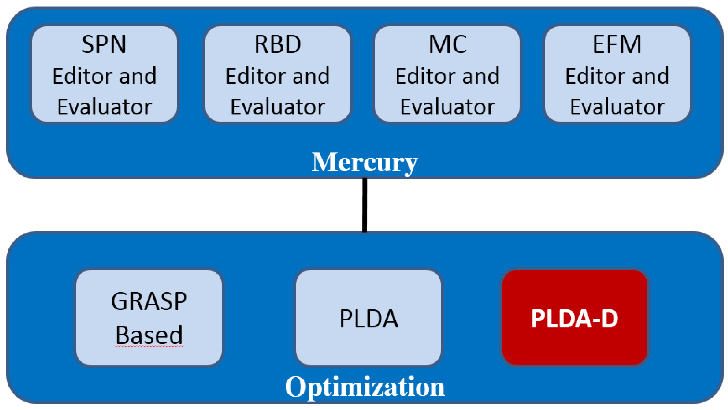
Both the proposed algorithm and the EFM model are supported in the Mercury modeling environment (see Section 4). In addition to the EFM model and the proposed algorithm, the Mercury environment also supports reliability block diagrams (RBD) [11], Markov chain [12] and stochastic Petri nets (SPN) [13] modeling, which are an essential part of the analysis. As such, the impact on the power subsystem reliability and availability was included.

The paper is organized as follows. Section 2 presents studies related to this research field. Section 3 introduces the basic concepts of the data center tier classification, sustainability and dependability. Section 4 presents an overview of the Mercury evaluation platform. Section 5 describes the energy flow model (EFM). Section 6 explains the PLDA-D. Section 7 describes the basic models adopted. Section 8 presents a case study, and finally, Section 9 concludes the paper and suggests directions for future work.

2. Related Works

Over the last few years, considerable research has been conducted into energy consumption in data centers. This section presents studies related to this research field.

Al-Fares [14] proposed an engine, called Hedera, for dynamic re-routing of the traffic of networking switch topologies that compose data center infrastructures. The main goal is to optimize the network bandwidth utilization with the proposed scheduler engine that has a minimal overhead on the available flows. Following the proposed approach by the authors, the bandwidth utilization was optimized to over 113% in relation to the static load-balancing strategies.

Dzmitry [15] proposed a methodology, named “Data center energy-efficient network-aware scheduling" (DENS) to manage job performance, energy consumption and data traffic. This proposed strategy is able to dynamically analyze the network feedback and make decisions to improve performance, energy consumption and the traffic. Therefore, the goal is to conduct the balance between those metrics, as well as to minimize the number of computing servers required on the data center that provide support to the services contracted.

These two papers are complementary to ours, as we propose a solution to reduce the energy consumption through the IT equipment of a data center, and those papers reduce the energy consumption by improving the network utilization.

Doria [16] extended the PowerFarm software [17] concept by adding an online monitor of loads and the correspondent power consumption. Additionally, the proposed EnergyFarm tool is able to turn off/on servers as needed according to the demands and respecting logical and physical dependencies. Therefore, the EnergyFarm turns off a set of servers to satisfy the required demand for storage on the data center, which reduces the overall system energy consumption, CO₂ emissions and the respective associated cost.

Heller et al. [18] proposed an engine, named ElasticTree, for managing the power consumption of computer networks. The ElasticTree is able to dynamically adjust switches in order to couple with the changes of the traffic loads of data centers. The main goal is, besides reducing the energy consumption, to improve performance and the fault tolerance of the system under analysis as well. To accomplish this, methods (e.g., formal models, greedy bin-packer, heuristic and prediction methods) are proposed to decide which links and/or switches must be used.

Neto et al. [19] proposed an algorithm, named MtLDF, to improve the load balance of fog systems considering performance metrics such as delay and priority. The authors have shown, through applied case studies, that the proposed method is able to reduce the energy consumption by improving the load distribution.

These previous related works are similar to the proposed strategy of our paper. However, none of them propose our own algorithm to minimize the energy consumption of the data center. The PLDA-D proposes the use of a new algorithm, based on the classic algorithms of minimum and maximum flow, making a mixture of both and obtaining a great result, with the search in depth.

3. Basic Concepts

This section discusses the basic concepts needed for a better understanding of the paper and presents an overview of the data center tier classification, followed by concepts regarding sustainability and combinatorial and state-based models. Finally, the concepts of Mercury environment and energy flow model are introduced.

3.1. Tier Classification

A data center infrastructure can be classified based on its redundancy features and fault tolerance ability [7]. This classification provides metrics to data center designers that identify the performance of the electrical infrastructureand strategies adopted. The following lines provide an overview of the four-tier classification.

3.1.1. Data Center Tier I (Basic)

This is a data center that does not offer redundant power and cooling infrastructures. A Tier I data center provides infrastructure to support information technology beyond office hours. Its infrastructure includes a dedicated area for the IT subsystem; a power subsystem with one uninterruptible power supply (UPS) to cope with power spikes and short outages; a dedicated cooling subsystem that does not shut down during office hours; and a generator to protect IT subsystem outages. Figure 1 depicts an example of the power system infrastructure for the Tier I data center.

We discuss how to manage schemas and their evolution for the last two scenarios (static schema management is straightforward and ignored here).

3.1.2. Data Center Tier II (Redundant Components)

A Tier II data center incorporates redundant critical power and cooling components, but with a single power distribution infrastructure. This infrastructure supports planned maintenance activities without interrupting the service, reducing as a result the system downtime. The redundant components include power and cooling equipment, such as UPS, chillers, pumps and engine generators. Figure 2 depicts an example of the power subsystem infrastructure assuming the Tier II classification.

3.1.3. Data Center Tier III (Simultaneous Maintenance and Operation)

A Tier III data center does not require shutdowns for equipment replacement or maintenance. The Tier III configuration considers the Tier II arrangement including a redundant independent power path (as shown through Figure 3). Therefore, each power component may be shutdown for maintenance without impacting the IT system’s operation. Similarly, a redundant cooling subsystem is also provided. These data centers are not susceptible to downtime for planned activities and accidental causes. Planned maintenance activities may be carried out using the redundant components and capabilities of the reference distribution so as to ensure the safe operation of the remaining components.

3.1.4. Data Center Tier IV (Fault-Tolerant Infrastructure)

A Tier IV adopts the Tier III infrastructure by adding a fault-tolerant mechanism, in which independent systems (electrical and cooling) are present. This tier classification is suitable for international companies that provide 24/7 customer services (as shown through Figure 4).

3.2. Sustainability

The concept of the green data center is related to electricity consumption and CO₂ emissions, which depend on the utility power source adopted. For example, in Brazil, 73% of electrical power is derived from clean electricity generation [8], whereas in the USA, 82.1% of generated electricity comes from petroleum, coal or gas [20]. Figure 5 depicts the relationship between the type of material used for power generation in Brazil and the USA.

Several methods and metrics are available for comparing equipment from a sustainability viewpoint.

Exergy is a metric that estimates the energy consumption efficiency of a system. It is defined as the maximal fraction of latent energy that can be theoretically converted into useful work [21].

$$Exergy=Energy\times F$$

(1)

where F is a quality factor represented by the ratio of $Exergy/Energy$. For example, F is 0.16 for water at 80 ${}^{°}$C, 0.24 for steam at 120 ${}^{°}$C and 1.0 for electricity [21].

The PUE (power usage efficiency) is defined as the total load of the data center ($C_{infrastructure}$) divided by the total load of the IT equipment installed ($C_{TI}$).

$$PUE=\frac{C_{infrastructure}}{C_{TI}}$$

(2)

3.3. Combinatorial and State-Based Models

RBD [22], fault trees [11], SPNs [23] and Continuous Time Markov Chains (CTMC) [12] have been used to model fault-tolerant systems and to evaluate some dependability measures. These model types differ in two aspects, i.e., simplicity and respective modeling capability. RBD and fault trees are combinatorial models, so they capture conditions that make a system fail in the structural relationships between the system components. They are more intuitive to use, but do not allow one to express dependencies between system’s components. CTMC and SPN models represent the system behavior (failures and repair activities) by its states and event occurrence expressed as labeled state transitions.

These state-based models enable the representation of complex relations, such as active redundancy mechanisms or resource constraints [22,24]. The combination of both types of models is also possible, allowing one to obtain the best of both worlds, via hierarchical modeling. Different model types can be combined with different levels of comprehension, leading to composite hierarchical models. Heterogeneous hierarchical models are being used to deal with the complexity of systems in other domains, such as sensors networks, telecommunication networks and private cloud computing environments.

3.3.1. Reliability Block Diagram

The reliability block diagram (RBD) [25] is a technique for computing the reliability of systems, using intuitive block diagrams. The RBD is able to represent the component’s interaction and to verify the relationship over the failed and active status of elements that keeps the system operational.

Figure 6a depicts a series relationship, where the system fails by the failure of a single component. Considering n independent components, the reliability is obtained by Equation (3)

$$\begin{array}{c}\hfill P_s=\prod _{i=1}^m\left(P_i\right)\end{array}$$

(3)

where P${}_i$ is the reliability—R${}_i$(t) (instantaneous availability (A${}_i$(t)) or steady state availability (A${}_i$))—of block b${}_i$.

Figure 6b shows a parallel arrangement, where the system continues to be operational, even with the failure of a single component. Considering n independent components, the reliability is obtained by Equation (4):

$$\begin{array}{c}\hfill P_p=1-\prod _{i=1}^m(1-P_i)\end{array}$$

(4)

For other examples and closed-form equations, the reader should refer to [11].

3.3.2. Stochastic Petri Nets

The Petri net (PN) [26] is able to represent concurrency, communication mechanisms, synchronization and a natural representation of deterministic and probabilistic systems. PN is a graph, in which places are represented by circles and transitions are shown as rectangles. Directed arcs are used to connect places and transitions and vice versa.

This paper considers stochastic Petri nets for conducting dependability analysis of data center power architectures. Figure 7 represents the SPN model of a “simple component”, where the places’ states are $X\_ON$ (activity) and $X\_OFF$ (inactivity). When the number of tokens (#) in the place $X\_ON$ is greater than zero, this means the component is operational. Otherwise, the component has failed. MTTFand MTTRof the system are used to compute the availability, and these parameters are not shown in the figure, but are associated with the transitions $X\_Failure$ and $X\_Repair$.

The expression IF ($\#X\_Rel\_Flag=1):2$ ELSE 1 defines the multiplicity (〈〈 md 〉〉), represented by the arc from $X\_OFF$ to $X\_Repair$. The place $X\_Rel\_Flag$ is adopted to let one conduct the evaluation of availability or reliability according to the marking of the place p. $\#XRel\_Flag=1$ means the reliability model is set; otherwise, we have the availability model.

If the number of tokens in the place is zero ($X\_Rel\_Flag$ and ($\#X\_Rel\_Flag=0$)), the probability P$\#X\_ON$ > 0 computes the component’s availability. Otherwise, ($\#X\_Rel\_Flag=1$); then the probability $P\#X\_ON>0$ allows one to compute the component’s reliability. That enables us to parameterize the model, allowing the system evaluation, considering or not the repair.

3.3.3. Continuous Time Markov Chains

Markov chains can be adopted to analyze various types of systems. A Markov process does not have memory; therefore, it has no influence from the past. The current state is enough to know the future steps. A Markov chain occurs when the process has a discrete state space. These states represent the different conditions that the system may be in. The events are represented by the transitions between the states.

In Figure 8, a new task is represented by the arc with rate $\lambda$. The arc with rate $\mu$ represents the server. This model depicts a system with two servers that compute received jobs. Considering the number of busy servers as a time function, it is possible to assume the function $X\left(t\right)$ or a random variable. The state $X_n\left(t\right)$ is named as any modification of X over $\left(t\right)$. The state space of the model is the set of all possible states. Therefore, we can compute the transition probabilities from a state to its successor $X_{n+1}\left(t\right)$.

In order to accomplish this, it is necessary to define the probability distribution function of $Xn\left(t\right)$. Stochastic processes are these random functions of time, where this variable changes its state over time [22].

4. Mercury

The Mercury environment [27,28] was developed by the MoDCS [28] research group for building and evaluating performance and dependability models. The proposed environment can be adopted as a modeling tool for the following formalisms: CTMC [12], RBD [11], EFM [9] and SPN [13,29,30].

Mercury offers useful features that are not easily found in other modeling environments, such as:

• More than 25 probability distributions supported in SPN simulation;
• Sensitivity analyses of CTMC and RBD models;
• Computation of reliability importance indices; and
• Moment matching of empirical data

Figure 9 details the functionalities available in the Mercury environment. The optimization module is able to evaluate the supported models (SPN, RBD, CTMC and EFM) through optimization techniques. In our previous study, we implemented GRASP (Greedy Randomized Adaptive Search Procedure) [31] and PLDA [9]. This paper proposes the PLDA-D as a great improvement over the PLDA. This is because in a single search, the PLDA-D considers two criteria for stopping, i.e., minimum flow for the lowest cost (Bellman) and maximum flow for energy (Ford–Fulkerson), with a scan of the graph in depth for each possible path.

5. Energy Flow Model

The EFM represents the energy flow between the components of a cooling or power architecture, considering the respective efficiency and energy that each component is able to support (cooling) or provide (power). The EFM is represented by a directed acyclic graph in which components of the architecture are modeled as vertices and the respective connections correspond to edges [8,32]. For more details about the formal definitions of the EFM, the reader is redirected to [32].

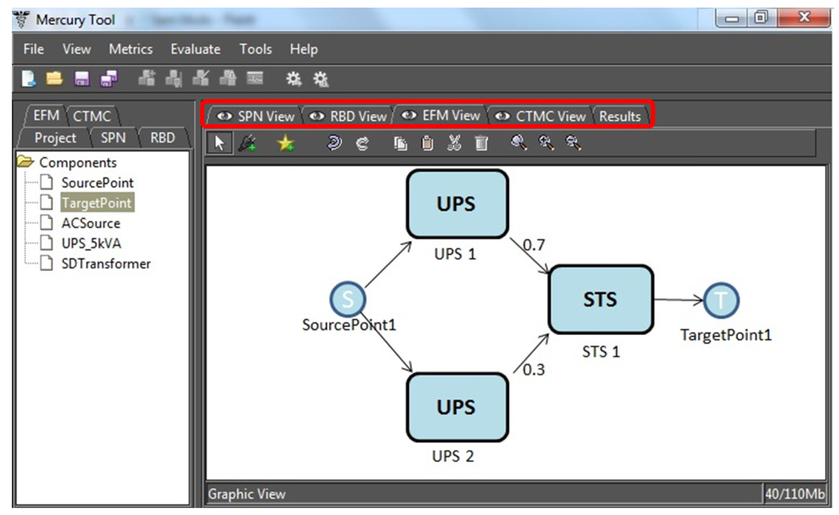
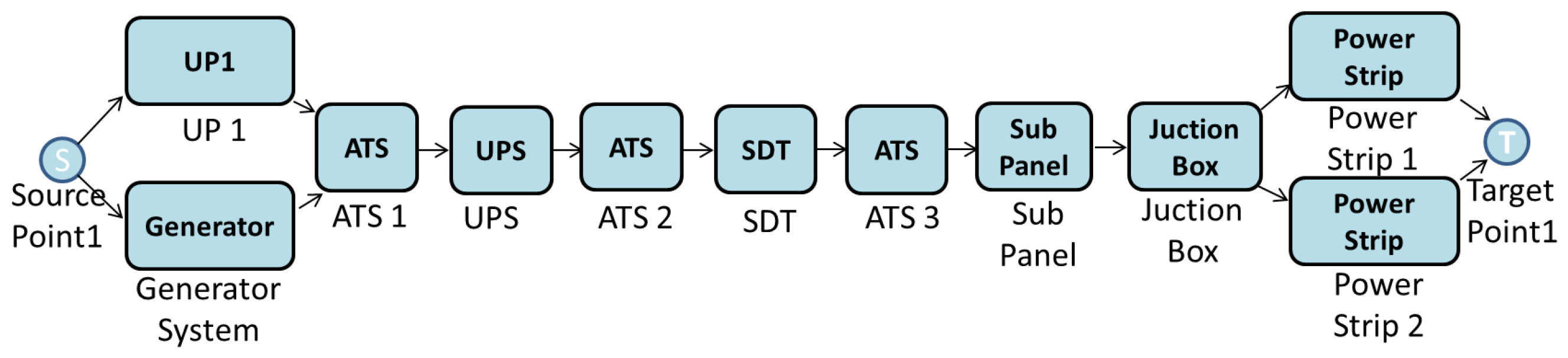
An example of EFM is shown in Figure 10. The rounded rectangles equate to the type of equipment, and the labels name each item. The edges have weights that are used to direct the energy that flows through the components. For the sake of simplicity, the graphical representation of EFM hides the default weight of one.

TargetPoint1 and SourcePoint1 represent the IT power demand and the power supply, respectively. The weights of the edges, i.e., 0.7 and 0.3, are the energy flows via the uninterrupted power supply (UPS) units, UPS1 at 70% and UPS2 at 30%, respectively, for meeting the power demand from the IT system.

The EFM is employed to compute the overall energy required to provide the necessary energy at the target point. If we consider that the demand from the data center computer room is 100 kW, this value is thus associated with TargetPoint1. Assuming that the efficiency of STS1 (static transfer switch) is 95%, the electrical power that the STS component receives is 105.26 kW.

A similar strategy is adopted for components UPS1 and UPS2, however now, dividing the flow according to the associated edge weights, 70% (73.68 kW) for UPS1 and 30% (31.27 kW) for UPS2. Thus, the UPS1 needs 77.55 kW, considering 95% efficiency, and UPS2 needs 34.74, considering 90% electrical efficiency. The Source Point1 accumulates the total flow (112.29 kW).

The edge weights are specified by the designer of the model, and there is no guarantee that the best values for the distribution were defined; as a result, higher power consumption may be reached. This work aims at solving such an issue by automatically setting the edge’s weight distribution of the EFM model with the PLDA-D algorithm. Therefore, our approach is able to achieve lower power consumption for the system.

Cost

In this paper, the operational cost considers the data center operation period, energy consumed, energy cost and the data center availability. Expression (5) denotes the operational cost.

$$OpCost=P_{Input}\times C_{Energy}\times T\times (A+\alpha (1-A))$$

(5)

$P_{input}$ is the power supply input; $C_{energy}$ is the energy cost per energy unit; T is the considered time period; A is the system availability; $\alpha$ is the energy percentage that continues to be consumed when the system fails.

6. Power Load Distribution Algorithm in Depth Search

The power load distribution algorithm-depth (PLDA-D) is proposed to minimize the electrical energy consumption of the system represented through EFM models [32]. PLDA-D is a depth search extension of PLDA [9,10]. The Bellman–Ford algorithm [33] is used for searches of the smaller path in a weighted digraph, whose edges have a weight, including a negative one. The Ford–Fulkerson algorithm [34] is used when it is desired to find a maximum flow that makes the best possible use of the available capacities of the network in question. The PLDA-D is a blend of these algorithms since it uses the characteristics of Bellman–Ford to choose the lowest cost, considering the weights of each node and the attributes of Ford–Fulkerson to pass the more significant amount of energy by a specific path, considering the energy efficiency of each piece of equipment.

The time and space analysis of depth-first-search (DFS) differs according to its application area. DFS traverses an entire graph with time $\Theta$ (|V| + |E|), linear in the graph size. In the worst case, it adopts the space O(|V|) to store the set of vertices on the actual search path like the stack of vertices visited [35]. Thus, in this setting, the time and space bounds are the same as for breadth-first search, and the choice of which of these two algorithms to use depends less on their complexity and more on the different properties of the vertex orderings the two algorithms produce.

In this case, for the properties of a data center’s electrical infrastructure, the depth search implemented in PLDA-D offers an optimal solution, whereas the width search performed in PLDA guarantees only a good solution.

The PLDA-D is divided into three phases: initialization, kernel calculations and search.

6.1. Initialization

This phase initializes variables, calls PLDA-D and computes the input power assigned to the EFM. In Algorithm 1 (initialize PLDA-D), the power infrastructure is represented by graph G (EFM model). Variable R stores a copy of G, so the original EFM is preserved (Line 1). The accumulated cost ($AccumCost$) of the variables, the capacities of the equipment ($cc{u}_v$), edge weights ($weig{h}_e$) and the input power ($inputPower$) are initialized with values of zero (Lines 2–11).

Algorithm 1 Initialization PLDA-D (G).

1: R = G; 2: for $v\in$ R do 3:   $cc{u}_v=0;$ 4:   $ActualCos{t}_v=\infty$ 5:   $AccumCos{t}_v=0;$ 6:   $Chil{d}_v=null$ 7: end for 8: for $e\in$ R do 9:   $weig{h}_e=0;$ 10: end for 11: $inputPower=0;$ 12: for $t\in$ $V_{target }$ do 13:   $R=PLDADKernel(R,f_d\left(t\right),s);$ 14: end for 15: $setUpdateWeight\left(R\right);$ 16: $\mathbf{return}$ $R;$

$ActualCos{t}_v$ of each node is initialized with a symbol denoting an infinite quantity (Line 4), and the variable $Child$ is initialized with a null value. This variable is adopted to create a relationship between nodes (Line 6).

Lines 12–14 call the PLDA-D function for each target node vertex (if there is more than one target in the EFM). The number of calls corresponds to the number of target nodes on G. If there is more than one target node, the energy flow will be distributed considering each.

The EFM edge weights are updated considering the accumulated flow of each component (Line 13).

6.2. Kernel Calculations

The kernel calculations, depicted in Algorithm 2 (Algorithm 2: PLDA-D kernel calculations), execute a loop with two stop criteria. First, it is checked if the demand is higher than zero ($f_d\left(t\right)$ > 0) and if there is a valid path from $Target\left(t\right)$ node to $Source\left(s\right)$ node (isPathValid(R,t,s)), where t is target node and s is the source. A valid path is a path from one node to another where the electrical capacity of all components in this path is respected.

Algorithm 2 PLDA-D kernel calculations (R, $f_d$(t), t, s).

1: while ($f_d\left(t\right)$ > 0) & (isPathValid($R,t,s$)) do 2:   $P=getElementsFromBestPath\left(t\right);$ 3:   $pf=\infty ;$ 4:   for$i\in P$do 5:     $pf=getMinimumCapacity(pf,f{c}_{\left(i\right)}-cc{u}_{\left(i\right)});$ 6:   end for 7:   for$i\in P$do 8:     $cc{u}_i=cc{u}_i+pf;$ 9:     if $(f{c}_{\left(i\right)}-cc{u}_{\left(i\right)}=0$) then 10:      $i.reachedLimit\left(\right)$ 11:     end if 12:   end for 13:   $f_d\left(v\right)$ = $f_d\left(t\right)$ − $pf;$ 14: end while 15: return R

The function $getElementsFromBestPath\left(t\right)$ aims at finding the best path from the target to the source node, according to the efficiencies and respecting the capacity of each element. This function is explained in the following section.

The path is stored in list P (Line 2), then the infinity symbol is assigned to the variable pf (possible flow) (Line 3), which stores the possible energy flow in the path. In the first loop (Lines 4–6), pf receives the value returned from getMinimumCapacity() for each path (Line 5), which returns the lower value between the actual possible flow (pf) and the difference between the flow capacity supported by the node $f{c}_{\left(i\right)}$ and the actual flow $cc{u}_{\left(i\right)}$.

The smallest possible value is added to each node of the path. The second loop (Lines 7–12) stores the accumulated flow ($cc{u}_i$). The limit of each piece of equipment is respected ($i.reachedLimit\left(\right)$) (Line 10). In the next valid path query, those that possess a selected node as a limit reached will be disregarded.

The demanded energy of the target node ($f_d\left(t\right)$) is updated (Line 13), subtracting the previously transmitted flow from its values. The previous steps are repeated until all valid paths have been analyzed or there is no demand. Finally, residual graph R is returned (Line 15), and only the edge weights are changed from the original graph G.

6.3. Search

We proposed our own version of an algorithm to compute maximum and minimum flows, which was implemented based on the Bellman [33] and Ford and Fulkerson [34] algorithms. More detail is provided in this section.

All paths are traversed from the target to source node. A cost is assigned to each node (component); the lower the value, the better the path. Once the cost associated with each path is calculated, it is possible to direct the flow to the better paths in relation to the electrical energy consumption.

Algorithm 3 (Algorithm 3: best patch choice) shows a function, called “$getElementsFromBestPath$”, responsible for identifying the best path through the nodes $Target$ to $Source$. In the first execution, the value passed as a parameter (CurrentVertices) is the $Target$ node. $ListOfParents$ stores the list of nodes with one level of the current node precedence, i.e., the list of parents (Line 1).

Line 2 starts a loop to each node of the list of parents. The first step of the loop chooses one item of equipment from a list of parents to begin the procedure (Line 3). The order of choice does not influence the search. The limit of capacity is verified in Line 4. If the node has reached its capacity limit, the algorithm proceeds looking for other paths available.

Algorithm 3 Search getElementsFromBestPath(CurrentVertices).

1: $ListOfParents=getListofParentsFrom\left(CurrentVertices\right)$ 2: for $i\in ListOfParents.size$ do 3:   $CurrentParent=ListOfParents\left[i\right]$ 4:   if $CurrentParent.LimitNotReached\left(\right)$ then 5:    $newCost=1/(CurrentVertices.getAccumCost\ast (CurrentParent.efficiency/100\left)\right)$ 6:    if $CurrentVertices=Target$ then 7:     $CurrentParent.setActualCost\left(newCost\right)$ 8:     $CurrentParent.setChild\left(CurrentVertices\right)$ 9:     $CurrentParent.setAccumCost($ 10:     $CurrentParent.efficiency/100)$ 11:    else 12:     $\mathit{if}$$CurrentParent.ActualCost>CurrentVertices.getActualCost+newCost$$\mathit{then}$ 13:     $CurrentParent.setActualCost($ 14:     $CurrentVertices.getActualCost+newCost)$ 15:   $CurrentParent.setChild\left(CurrentVertices\right)$ 16:   $CurrentParent.setAccumCost($ 17:   $CurrentParent.efficiency/100)\ast CurrentVertices.getAccumCost$ 18:    end if 19:    $getElementsFromBestPath\left(CurrentParent\right)$ 20:   end if 21: end for 22: $ListOfElements.addBestChild\left(Source\right)$ 23: return $\left(ListOfElements\right)$

Line 5 computes the cost of each component node, in which the shortest value represents the best path choice. Line 6 verifies if the vertex under analysis (CurrentVertices) is the $Target$. In this case, the $CurrentParent$ cost receives $newCost$; the $CurrentVertices$ is assigned as the $Child$ of $CurrentParent$; and the accumulated cost is computed (Lines 7–9). The accumulated cost represents the cost of the node multiplied by the cost of the path that precedes it. This step draws the best path.

Assuming the $CurrentVertices$ are not the $Target$, Line 11 conducts a check that is only satisfied when there is at least one path with a lower cost to be reached.

In this case, the $CurrentParent$ cost is updated to the sum of the cost of the $CurrentVertices$ plus the $newCost$. The $CurrentVertices$ will be the “$best$ $child$” for the $CurrentParent$, and the $CurrentParent$ cost is updated considering this new path (Lines 12–14).

In Line 19, a list of elements is filled with the children of the $Source$ node, which corresponds to the best path from the $Target$ to the $Source$ node, according to the expression of Line 5. Finally, a list with the elements of the best path is returned (Line 20).

6.4. PLDA-D Execution

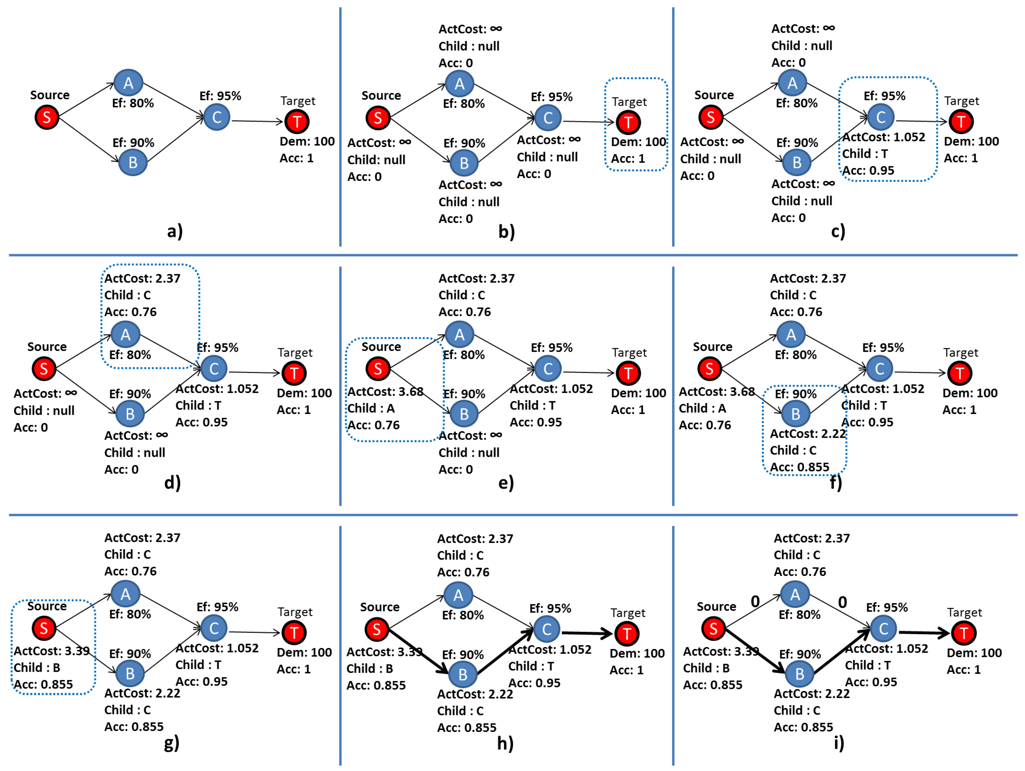
Figure 11 illustrates the step-by-step execution of the PLDA-D. Figure 11a shows an EFM composed of three electrical components A, B, and C, with an efficiency of 80, 90 and 95%, respectively. S is the $Source$ node, representing an electrical utility, and T is the $Target$ node, representing a computer room.

The demand ($Dem$) and the efficiency ($Ef$) values are specified by the data center designer. The $Target$ node $Acc$ value is set to one. The other accumulated costs ($Acc$) are set to zero, and the edge weights are set to the default value, respectively, as depicted in Figure 11a. Phase 1 of the PLDA-D is represented by Figure 11b, where all variables of all vertices are initialized.

Phase 2 starts in Figure 11c following until Figure 11h. The best path is selected according to the efficiency of each component. In Figure 11c, the values of the $ActualCost$ and $AccumulatedCost$ are computed, and the best child is chosen according to the lowest value of the variable $ActCost$.

Next, one of the parents of node C is chosen; the order of choice does not influence the search. Node A was selected, and the values of $Acc$ and $ActCost$ were computed; the best child is node C; see Figure 11d.

The values of $ActCost$ and $Acc$ were computed according to Equations (6) and (7), as described in Lines 5 and 14 of Algorithm 3.

$$ActCost=ActCost+\frac{1}{ActCost\times \frac{efficiency}{100}}$$

(6)

$$Acc=Acc\times \frac{efficiency}{100}$$

(7)

Figure 11e shows the algorithm step in which $Acc$ and $ActCost$ of all variables were computed and the best child selected. The $Source$ is a terminal node and has no parent; thus, the algorithm returns to the node C that has two parents. Node C has not been thoroughly researched, because there is an unvisited parent node B. Figure 11f shows the algorithm step once the variables for node B have been computed.

Figure 11g depicts the step after calculating variables $Acc$ and $ActCost$ and verifies that the $ActCost$ for the current path (3.39) was less than the $ActCost$ of the previous path (3.68) for reaching the $Source$ node. Thus, the $Source$ node has changed the values of its variables, and the best $Child$ is now node B and no longer node A. In other words, the path passing through the node B represents a better choice than passing through the node A.

Figure 11h represents the end of Phase 3, which returns the best path to Phase 2. The best path from the target to source node is: $Target, C, B,$$Source$. Figure 11i presents the flow distributed by Phase 2. After that, the EFM computes the minimum possible value for the input power.

7. Basic Models

This section presents the analysis of the proposed models for representing the previous four-tier configurations. The baseline architecture is modeled with RBD; however, RBD models cannot completely represent complex systems with dependencies between components.

State-based methods can represent these dependencies, thereby allowing the representation of complex redundant mechanisms. The Achilles heel for state-based methods is the exponential growth of the state space as the problem becomes large, which can either increase the computation time or make the problem mathematically intractable. However, strategies for hierarchical and heterogeneous modeling (based on states and combinatorial models) are essential to represent large systems with complex redundancy mechanisms [22]. MC, SPN, RBD and EFM models were utilized to evaluate the four tiers. The availability was obtained by the RBD, MC or SPN model. The other metrics (cost, PUE, input power) were achieved through the EFM evaluation.

7.1. Tier I Models

Figure 12 and Figure 13 depict the RBD models for power and cooling architectures of Tier I, respectively. The power and cooling architectures were evaluated separately.

After that, we assumed that the system was only operational once both the cooling and power system were working. Therefore, the previous availability results were put together in a serial relationship, meaning that the failure of an electrical device would also affect the cooling equipment. Moreover, the system availability was compared with the Up Time Institute [7], in which there can be no doubt that the results achieved are equivalent.

Once the availability was computed, the EFM shown in Figure 14 was adopted for computing, for instance, cost and operational exergy. Only the electrical infrastructure was consider in the EFM model.

7.2. Redundancy N + 1

Redundancy N + 1 is adopted in utility power and generator systems for Tiers II, III and IV. This redundancy is a form of ensuring system availability in the event of component failure. Components (N) have at least one independent backup component (+1). This paper considers redundancy $N+1$ (generator and UPS), as there is a demand for at least two pieces of equipment. One machine works with a spare backup; thus, N is assumed to be two.

The RBD model is used to obtain the dependability metrics of the electrical infrastructure of data center Tiers II, III and IV. However, due to the system complexity of the redundancy (N + 1), the utility power and generator subsystem were modeled in SPN (Figure 15 depicts the corresponding SPN model for that system). This model represents the operational mode of the utility power and generator system, in which the system is operational if the power supply utility ($\#C\_UP$ = 1) and the two main generators are operating ($\#G12\_Up$ = 2) or if one main generator and one backup is running, i.e., (($\#G12\_Up$ = 1) and ($\#Gb\_Up$ = 1)).

In this SPN model, the transaction that activate Generators 1 and 2 (G12 Act) is only fired when the power supply utility has failed. Similarly, the transaction $Gb$ $Act$ is able to fire once the power supply utility and at least one main generator have failed.

The availability expression obtained by the SPN model is:

$$\begin{array}{c}{\displaystyle A=(C_{U}p=1)OR(G{12}_{U}p=2)OR\left((G{12}_{U}p=1)AND(G{b}_{U}p=1)\right)}\hfill \end{array}$$

(8)

The UPS system is modeled with redundancy (N + 1), assuming a cold standby strategy. A cold standby redundant system considers a non-active spare component that is only activated when the main active component fails. The components of the UPS system are based on a non-active redundant module that expects to be active when the main module fails. The operational mode of this system considers that at least two UPSs must be active. Figure 16 depicts the Markov chain model adopted to evaluate the availability of the UPS system with redundancy (N+ 1) in cold standby.

In Figure 16, State 2 represents the two standard UPSs operating and the backup waiting. State 1 shows the detection of a fault in one UPS. State 2* represents two UPSs operating (one standard UPS and one backup). State 1* represents a fault in the standard or backup UPS. State 0 represents the fault of all the UPS’s. State 0* shows the fault of two standard UPSs and the operating of the backup. The failure rate is represented by $\lambda$; $\mu$ is the repair rate; $\sigma$ is the mean time to activate the backup UPS.

The availability expression obtained by the CTMC model is A’/A”, where:

$$A^{\prime }=\left(\mu \sigma (4{\lambda }^3+4{\lambda }^2(\mu +\sigma )+{\mu }^2(\mu +\sigma )+\lambda \mu (3\mu +2\sigma ))\right)$$

(9)

$$\begin{array}{c}{\displaystyle A^{″}=(2{\lambda }^2{\mu }^3+(\lambda +\mu )(2\lambda +\mu )(2{\lambda }^2+{\mu }^2)\sigma +(4{\lambda }^3+4{\lambda }^2\mu +2\lambda {\mu }^2+{\mu }^3){\sigma }^2)}\hfill \end{array}$$

(10)

7.3. Tier II Models

Availability results are obtained through the evaluation of these SPN models, as well as the RBD and MC. We use two-level hierarchical models in which RBD is used to represent the overall system on the upper level, and SPN and MC are used to capture the behavior of the subsystem on the lower level, as power and UPS systems. Figure 17 depicts the RBD model adopted to represent the power infrastructure.

The values of the GS + UP1 (Generator_System and UtilityPower1) and the UPS_System used in the RBD models of Tiers II, III and IV are computed through the SPN and MC models in Figure 15 and Figure 16, respectively. The availabilities of the SPN and MC models are computed and inserted into each block of the RBD (e.g., UP1 + GS) models.

Figure 18 depicts the EFM model of the electrical infrastructure of data center Tier II. As the reader may observe, there is a difference between the representation of dependability models and the electrical flow to the power strip component.

At first, representation in series signifies that the failure of one component affects the operation of the data center. In the second, the parallel representation signifies that the electrical flow is distributed by all power strip devices.

7.4. Tier III Models

The data center Tier III model uses hierarchy to represent the UPS system and power generation system. The Tier III model is divided into subsystems; two of them represent the power and UPS systems previously presented (Figure 15 and Figure 16). One path of the electrical flow uses the UPS system with redundant components (Subsystem X), and the other path has no redundant components (Subsystem Y). Both provide possible paths to the set of power strip components (Subsystem P). The availability algebraic expressions of each subsystem is shown in Equations (11)–(13).

$$\begin{array}{c}{\displaystyle SubsystemX=ATS1\times UPSSystem\times ATS2\times SDT1\times SubPanel1\times JuctionBox1}\hfill \end{array}$$

(11)

$$\begin{array}{c}\hfill SubsystemY=SDT1\times SubPanel2\times JuctionBox2\end{array}$$

(12)

$$\begin{array}{c}\hfill SubsystemP=\prod _{i=1}^n\left(PowerStri{p}_{\left(n\right)}\right)\end{array}$$

(13)

where n is six in this model. Equation (14) shows the algebraic availability expressions of all subsystem (X, Y, P) that compose Tier III.

$$\begin{array}{c}TierIII=(1-(1-(UPS\_GS)\times (ATS1\times UPSSystem\times ATS2\times SDT1\times \\ SubPanel1\times JuctionBox1\left)\right)\times (1-(UP2)\times (SDT1\times SubPanel2\times JuctionBox2\left)\right))\times \\ \left(\prod _{i=1}^n\left(PowerStri{p}_{\left(n\right)}\right)\right)\end{array}$$

(14)

Once availability is computed, the EFM model can be analyzed to provide cost and operational exergy, as well as to ensure that the power restrictions of each device are respected. Figure 19 presents the EFM model adopted for Tier III.

7.5. Tier IV Models

Tier IV is the highest level of assurance that a data center can offer. This data center category is fully redundant in terms of electrical circuits (see Figure 4).

The RBD of Tier IV is modeled using a similar approach to Tier III, with hierarchical models. Five subsystems are used, two representing the power and UPS system (Figure 15 and Figure 16). There are two redundant paths of electrical flow, both with redundant UPS systems. One path, named Subsystem Z (see the availability algebraic expression in Equation (15)), is composed of ATS1, UPS System 1, ATS2, SDT1, SubPanel 1and JunctionBox1. The set of power strips for data center Tier IV is present in Equation (16), where m is eight.

$$\begin{array}{c}\hfill SubsystemZ=ATS1\times UPSSystem1\times ATS2\times SubPane1\times JuctionBox1\end{array}$$

(15)

$$\begin{array}{c}\hfill SubsystemPS=\prod _{i=1}^m\left(PowerStri{p}_{\left(m\right)}\right)\end{array}$$

(16)

There are two utility powers, each with a backup generator system (UtilityPower1 + GeneretorSystem1 and UtilityPower2 + GeneretorSystem2). The availability algebraic expression of Tier IV is presented in Equation (17).

$$\begin{array}{c}TierIV=(1-(\prod _{i=1}^n(1-{(UtilityPower\_GeneretorSys)}_{\left(n\right)}\times (ATS1\times UPSSystem1\\ {\times SubPane1\times ATS2\times JuctionBox1)}_{\left(n\right)}\left)\right)\times \left(\prod _{i=1}^m\left(PowerStri{p}_{\left(m\right)}\right)\right)\end{array}$$

(17)

After computing the availability value of Tier IV, the EFM depicted in Figure 20 is adopted.

8. Case Study

The main goal of this case study is to validate the proposed models and to show the applicability of the PLDA-D algorithm, considering the data center power infrastructure of Tiers I, II, III and IV. To conduct the evaluation, the environment Mercury was adopted. In addition to computing the dependability metrics, Mercury is adopted for estimating the cost and sustainability impact, as well as to conduct the energy flow evaluation and propose a new one, according to the optimization of the PLDA-D algorithm. 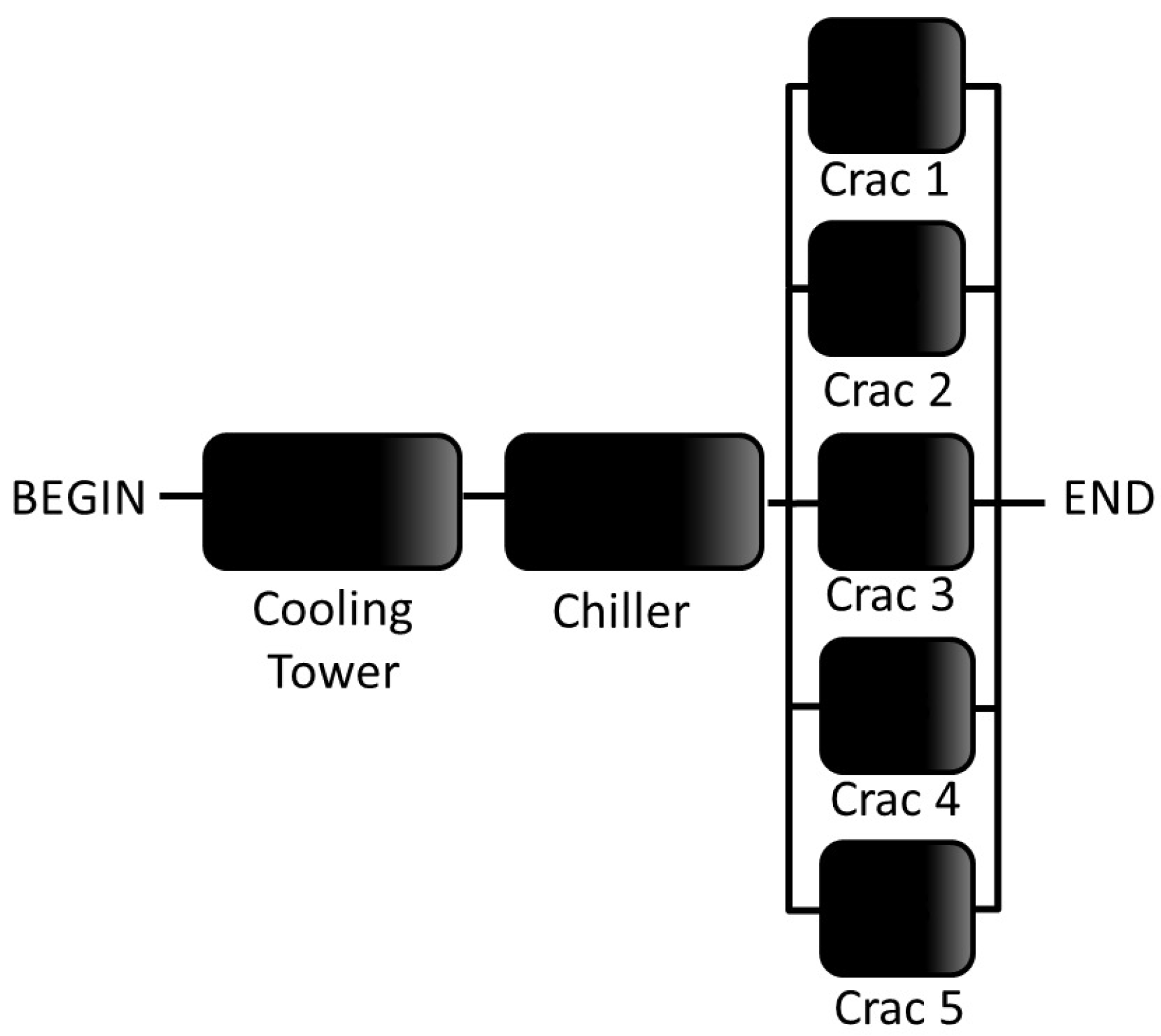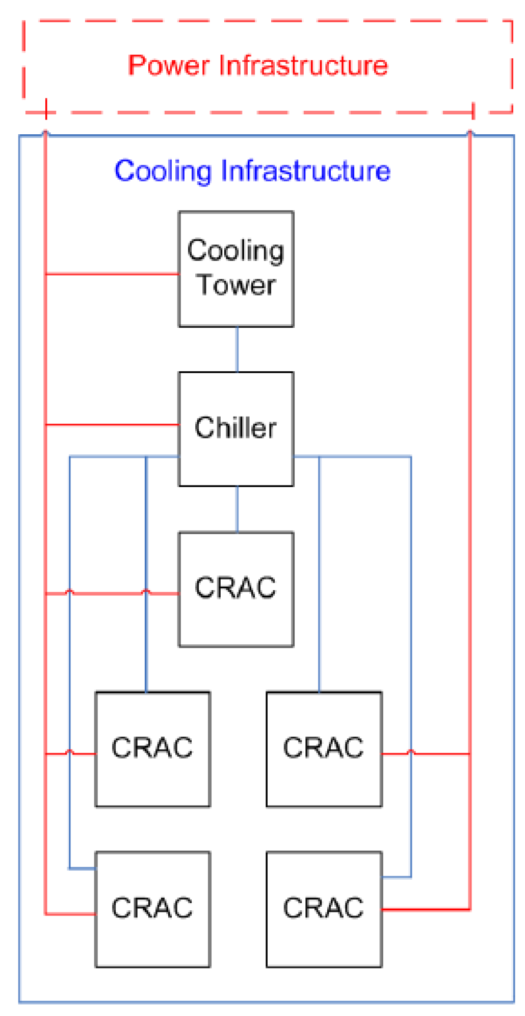Figure 21 depicts the connections between cooling components and electrical infrastructure.

To validate the Tier I model, the cooling and power infrastructure were evaluated together. The value of the availability proposed for Tier I according to the Up Time Institute is 0.9967. The availability obtained from the RBD model of Figure 12 and Figure 13 was 0.9952. To validate the proposed model, the relative error was used, to compare the difference between the results. Considering the relative error (presented in Equation (18)), the value of 0.0015 was reached.

$$RelativeError=\frac{(Theoretical-Experimental)}{Experimental}$$

(18)

A very small value for the relative error was found; therefore, we consider the proposed model to be an accurate representation of the Tier I model. The same strategy was adopted to validate the other proposed models of Tiers II, III and IV.

Table 1. MTTRand MTTRvalues.

Equipment	MTTF (h)	MTTR (h)
AcSource	5380.0	8
Generator	3190.0	8
ATS	282,581	8
UPS	60,000	8
SDT	1,412,908	8
Subpanel	404,000	8
Junction Box	5,224,000	8
Power Strip	215,111	8
Cooling Tower	24,816	48
Chiller	18,000	48
CRAC	37,059	8

shows the MTTF and MTTR values for each device. These values were obtained from [36].

To show the applicability of the PLDA-D, four data center power infrastructure tiers were evaluated considering the following metrics: (i) total cost; (ii) operational exergy; (iii) availability; and (iv) PUE (power usage efficiency). These metrics were computed over a period of five years (43,800 h). Each metric was computed before and after the PLDA-D execution.

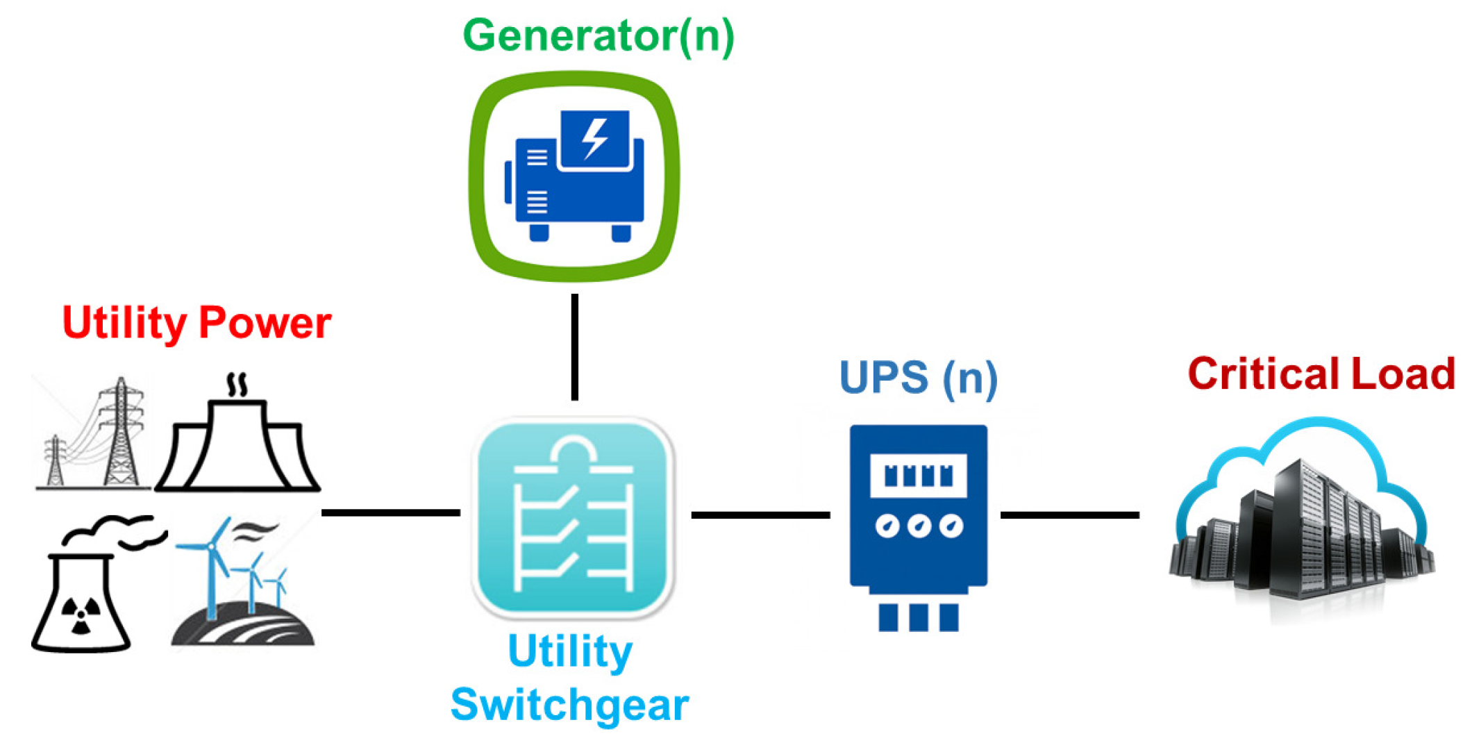
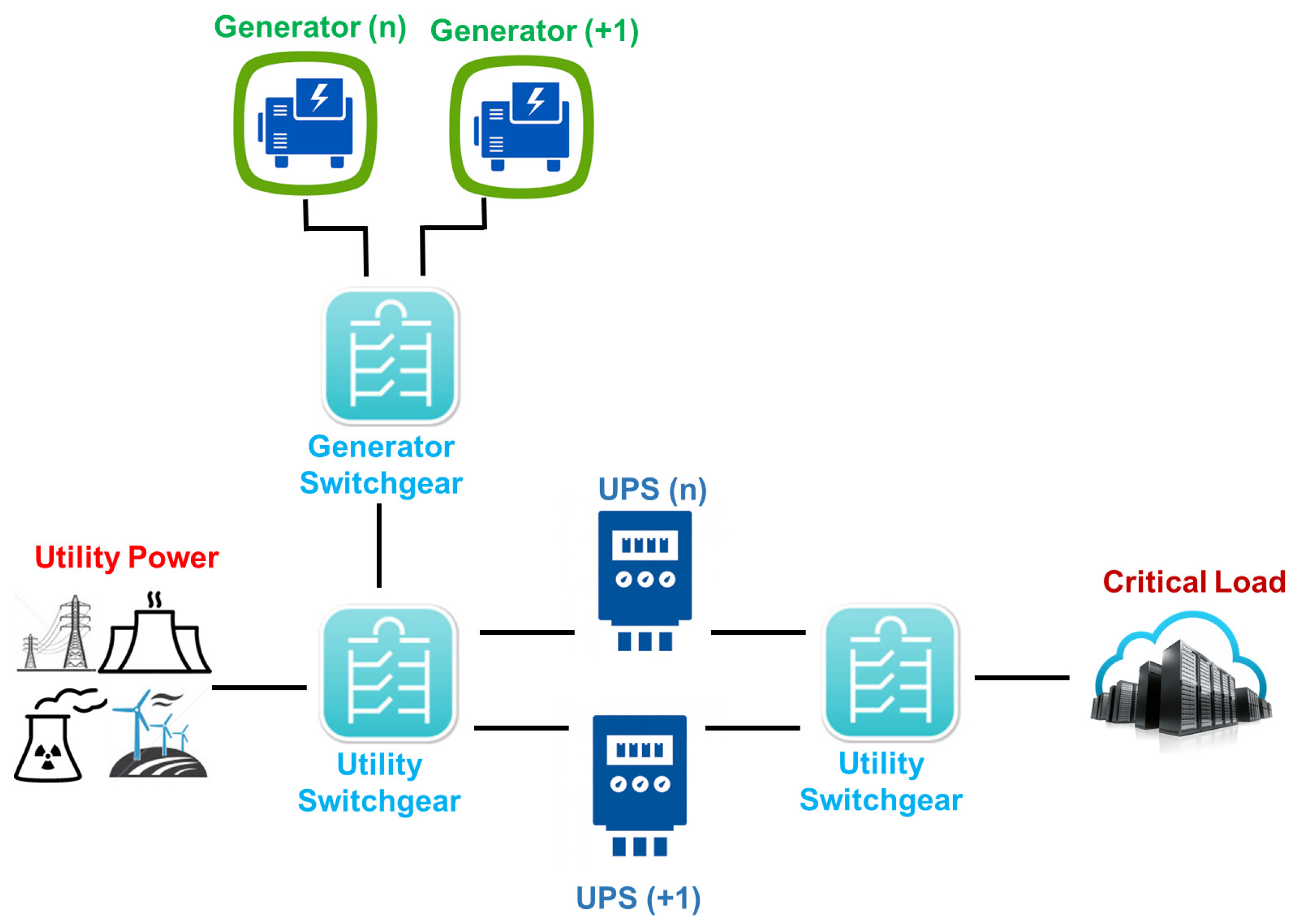
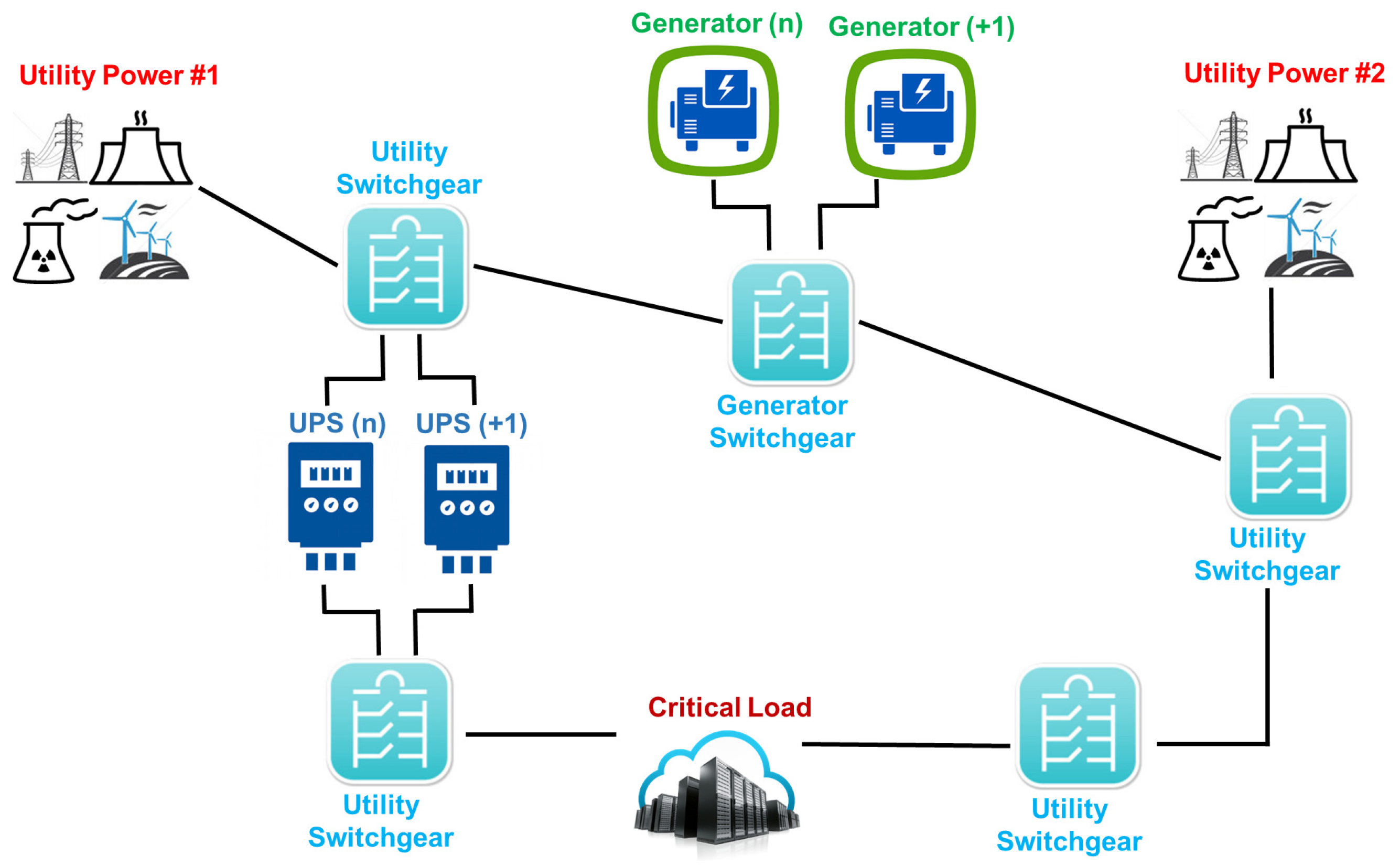
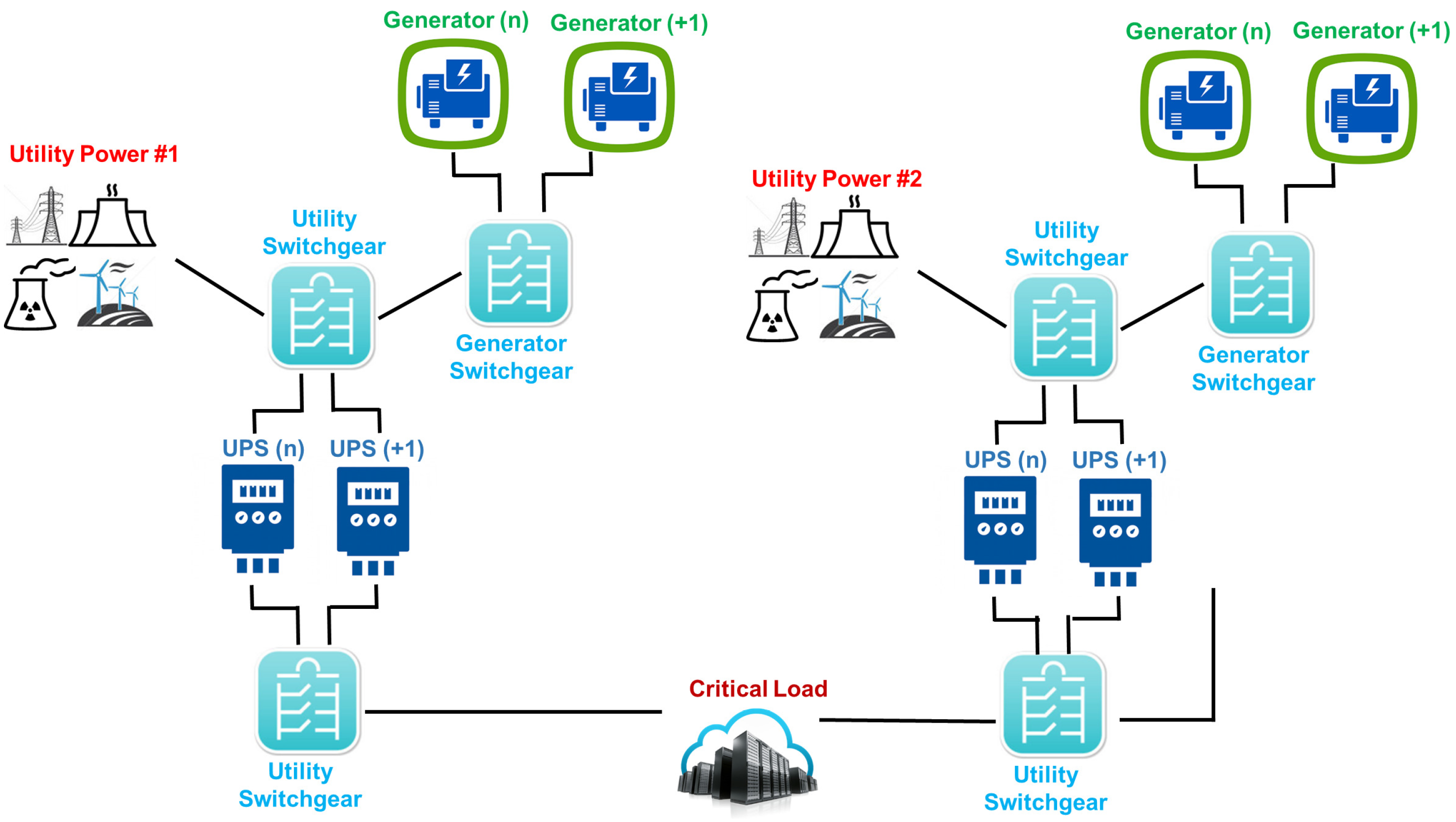
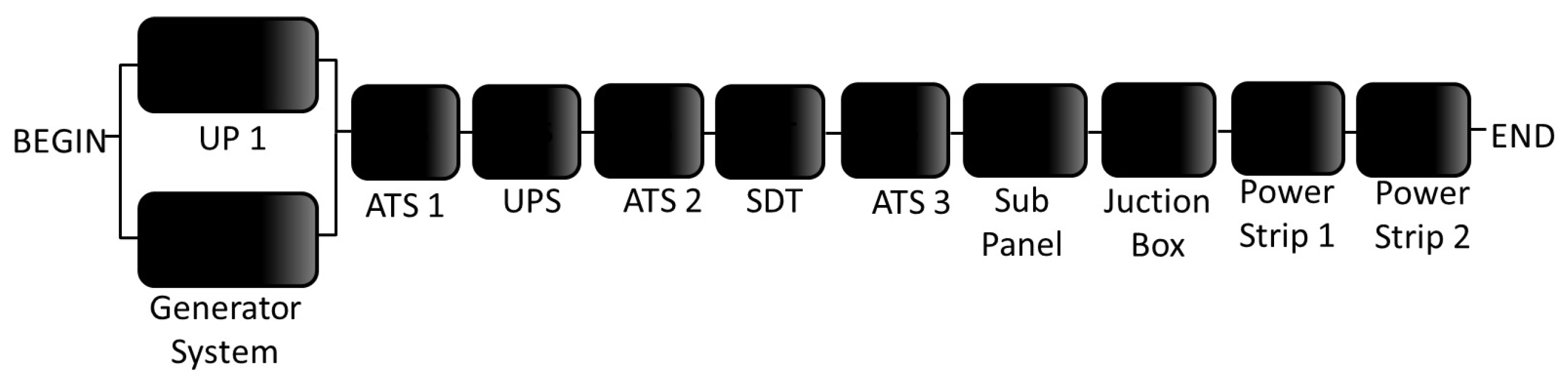
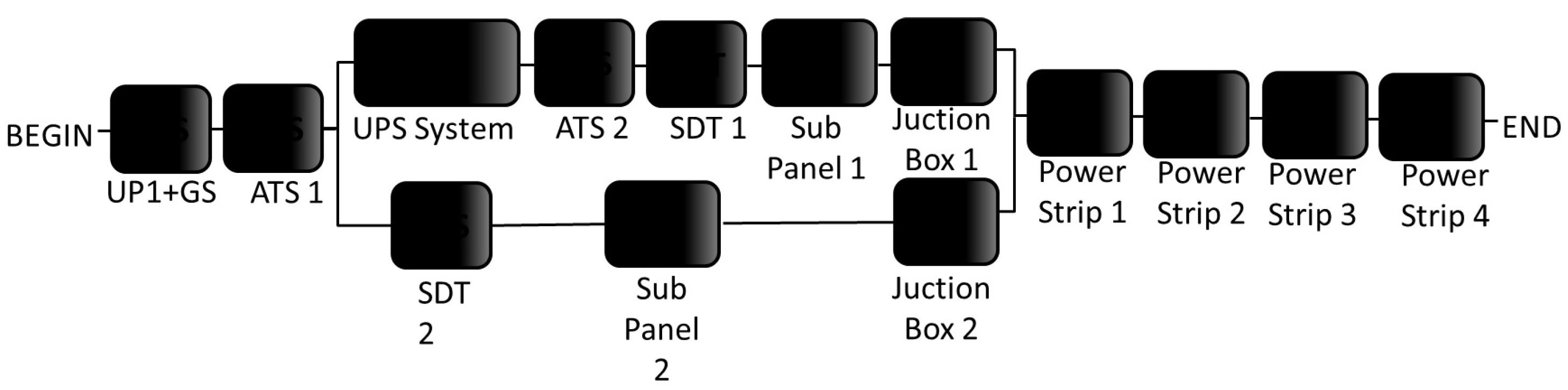
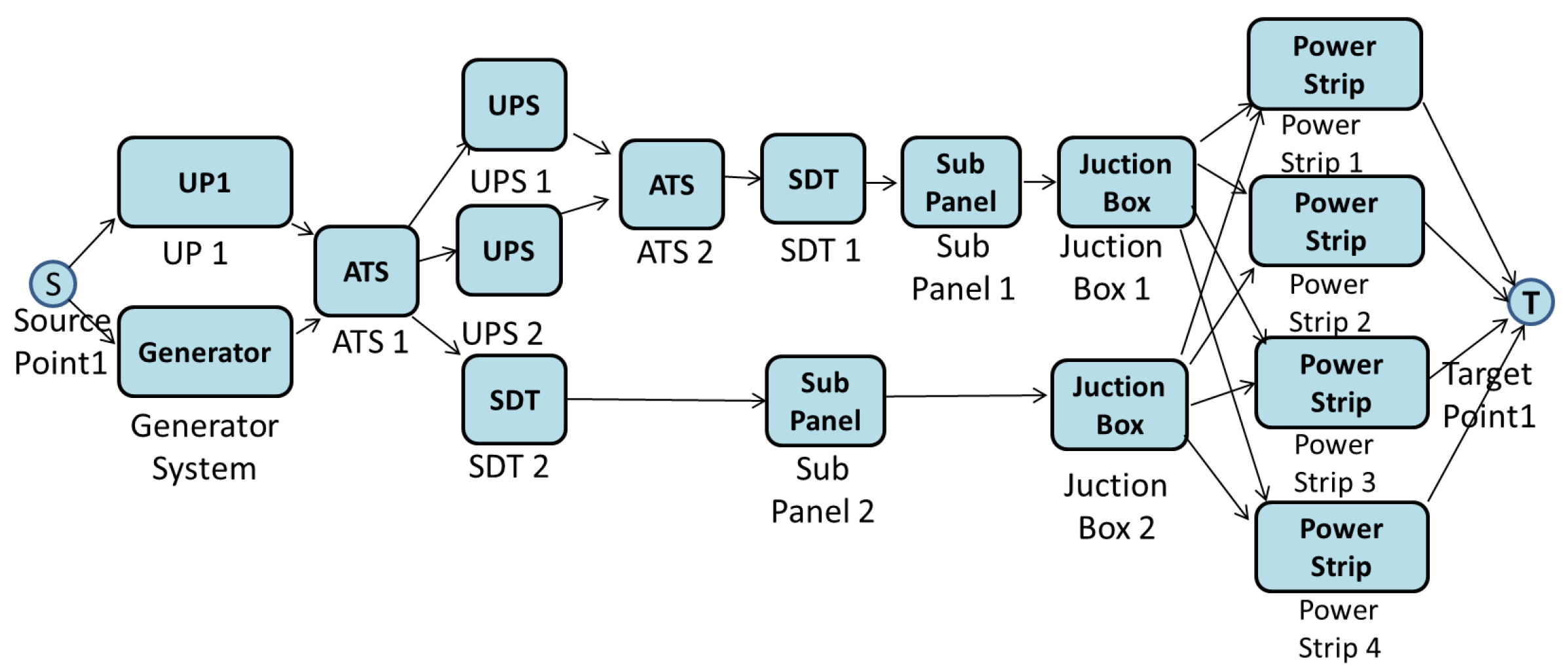
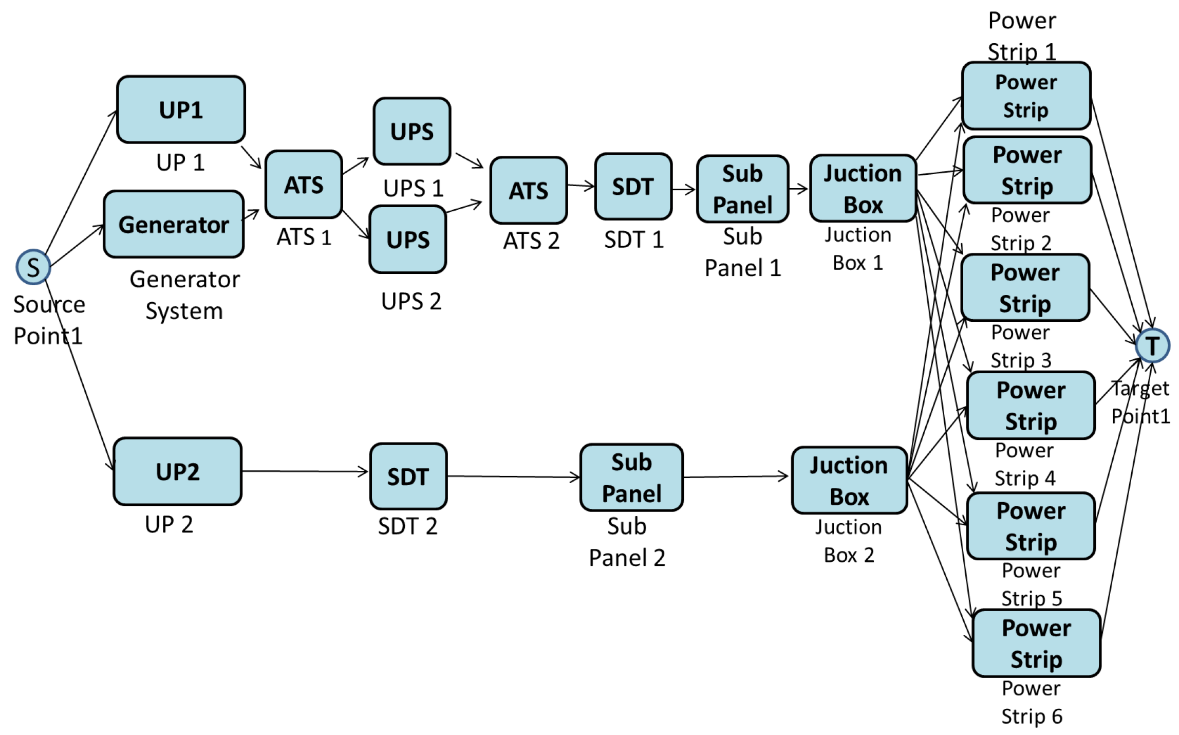
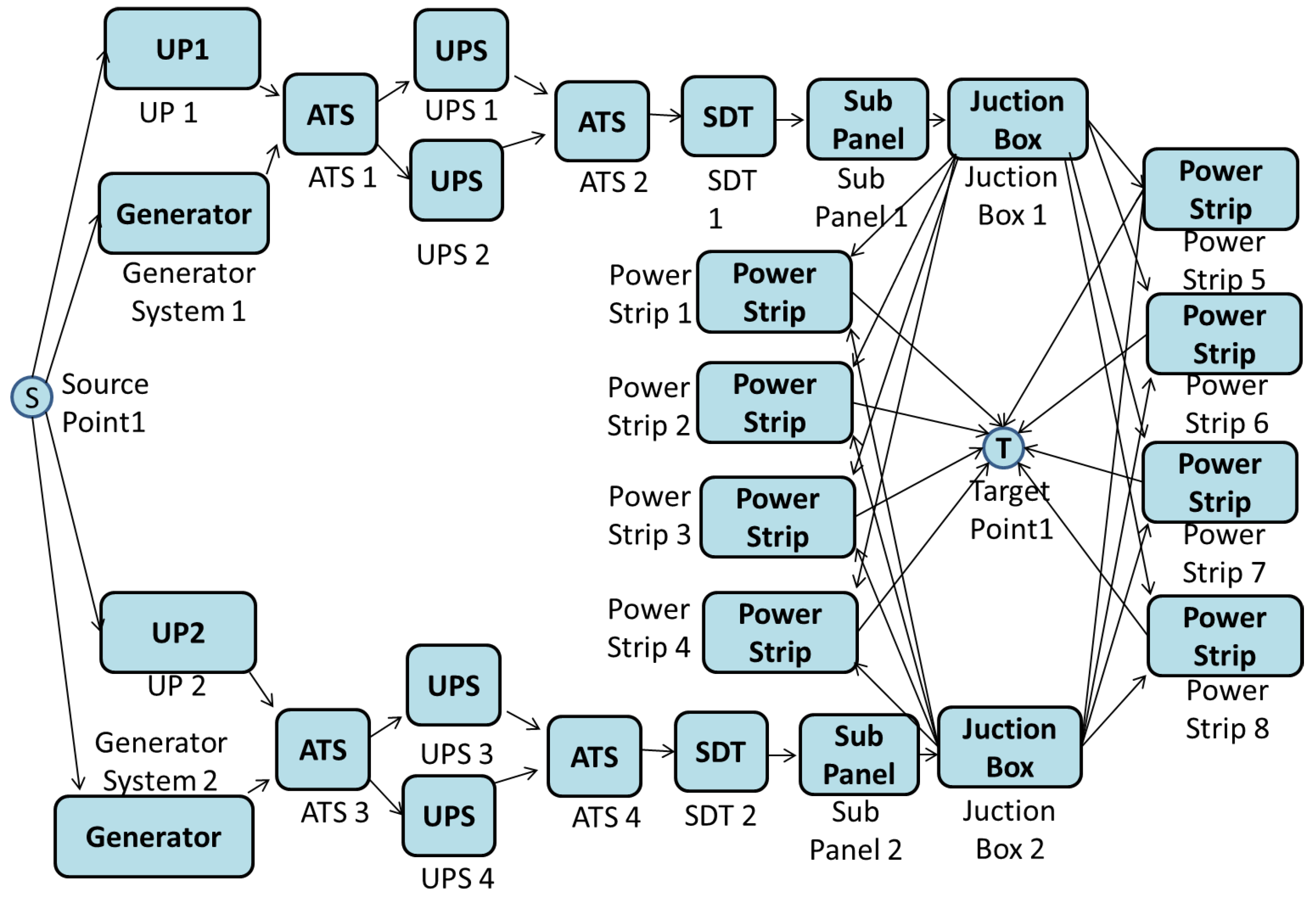
The electrical flow in a data center starts from a power supply (i.e., utility power), passes through uninterruptible power supply units (UPSs), the step down transformer (SDT), power distribution units (PDUs) (composed of a transformer and an electrical subpanel) and, finally, to the rack. According to the adopted tier configuration, different redundant levels were considered, which impact the metrics computed for this case study.

Table 2. Capacity and efficiency. SDT, step down transformer.

Equipment	Efficiency (%)	Capacity (kW)
Utility Power 1	95.3	10,000
Utility Power 2	90.0	10,000
STS 1	99.5	1500
STS 2	98.0	1500
SDT (or transformer) 1	98.5	5000
SDT (or transformer) 2	95.0	5000
Subpanel 1	99.9	1500
Subpanel 2	95.0	1500
UPS 1	95.3	5000
UPS 2	90.0	5000
Junction Box 1	99.9	1500
Junction Box 2	98.0	1500
Power Strip 1	99.5	5000
Power Strip 2	95.1	5000

presents the electrical efficiency and maximum capacity of each device.

Table 3. Results of PLDA-D execution with improvement in %. Operational Exergy, Total Cost; Availability and PUE.

Tiers	-	Oper. Exergy	Total Cost	Availability	PUE
Tier I	Before	4688	1,173,593	0.999605271	86.84 (%)
	After	4418	1,165,323	0.999605271	87.50 (%)
	Improvement (%)	6.13	0.71	0	0.77
Tier II	Before	10,127	2,289,365	0.9997510814	85.94 (%)
	After	8837	2,249,961	0.9997510814	87.50 (%)
	Improvement (%)	14.59	1.75	0	1.82
Tier III	Before	13,242	3,347,222	0.9999999380	87.52 (%)
	After	11,077	3,281,087	0.9999999380	89.34 (%)
	Improvement (%)	19.54	2.02	0	2.08
Tier IV	Before	16,252	4,452,412	0.99999993803	88.39 (%)
	After	11,000	4,291,925	0.99999993803	91.84 (%)
	Improvement (%)	47.75	3.74	0	3.9

summarizes the results for each power infrastructure of data center Tiers I–IV. Row $Before$ presents the results obtained before executing the PLDA-D; row After presents the results after PLDA-D execution; Improvement (%) is the improvement achieved as a percentage; Oper. Exergy is the operational exergy in gigajoules (GJ) (considering five years); Total Cost is the sum of the acquisition cost with the operation cost in USD (for five years); Availability is the availability level; PUE is the power usage efficiency as a percentage, which corresponds to the total load of the data center divided by the total load of the IT equipment installed.

We apply the PLDA-D algorithm to each EFM architecture, and as a result, the weights presented on each edge of the EFM model are updated, improving the energy flow. The lowest value of the input power is reached, and thus, all metrics related to energy consumption are improved.

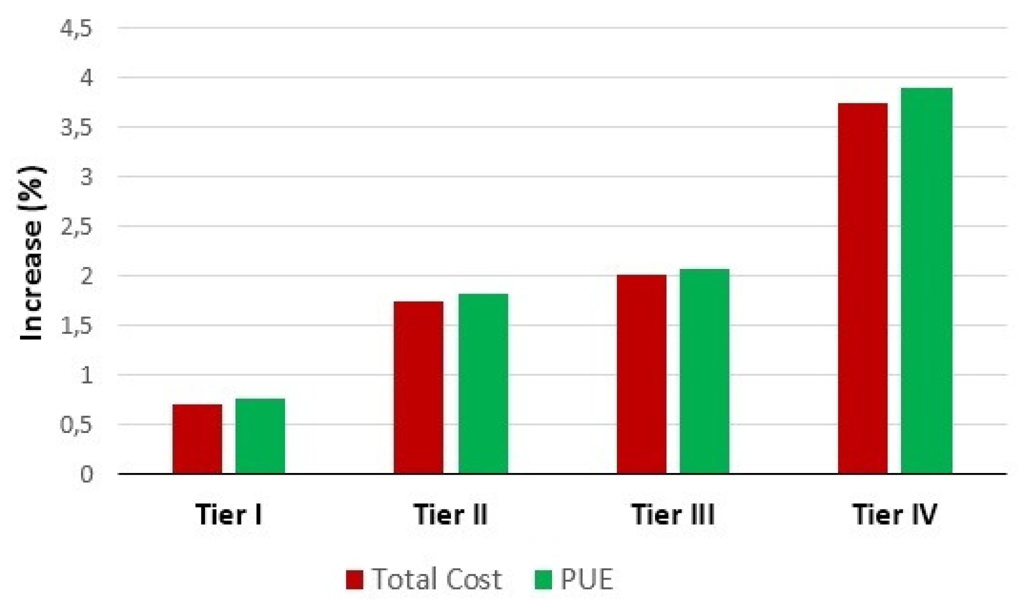
From the aforementioned table, the first observation to be noted is the improvement obtained after using the PLDA-D algorithm. The metrics of sustainability, energy consumption and cost are all improved. For instance, even in the data center of Tier I, where no redundant components are considered, improvements were achieved. For instance, the operational exergy was reduced by 6.13% and the total cost by 0.71% (which corresponds to 8720 USD savings), and the PUE metric was also improved by around 0.77%.

Tier II presents an improvement in cost and sustainability metrics. For example, operational exergy was reduced from 10,127 to 8,837 GJ and PUE from 85.94 to 87.50 (%), and the cost improved by 1.75 (%), which would be 39,404 USD. Assuming Tier III, a reduction of almost 20% was observed in operational exergy and 2% in total cost, which in financial resources equates to 66,135 USD. The PUE was improved by 2.08%, reaching 89.34%, a considerable improvement.

The data center classified as Tier IV is the most complete in redundancy and security levels. The values achieved were significant, with a reduction of almost 50% in operating exergy and almost 160,500 USD in five years. The PUE was improved by 3.9%. Figure 22 presents the increase of the total cost and PUE.

Although the improvements to the algorithm seem slight, the long-term values are high. For instance, the total cost of Tier II was 1.75 (%), which means USD 39,403 over five years. Resources from these energy savings could be used for hiring employees, team qualification or acquiring equipment. In order to do this, it is sufficient to adopt a new method for distributing the electrical flow.

Furthermore, the UPS system is responsible for maintaining the IT infrastructure; then, there is a relationship between the tier classification and the capacity of the UPS system. The average power consumption of a computer room according to the tier level is shown in

Table 4. Relation between cost/kW before/after PLDA and PLDA-D.

Tier Classification	Cost/kW	After PLDA	After PLDA-D
Tier 1	10,000	9923	9923
Tier 2	11,000	10,870.2	10,870.2
Tier 3	20,000	19,679	19,584
Tier 4	22,000	21,337	21,142

[37].

The columns “After PLDA” and “After PLDA-D” represent the results achieved after running the PLDA and PLDA-D algorithms, in which a reduction in comparison with the average power consumption (column “Cost/kW”) can be noticed.

To compare the improvement of PLDA-D also with its predecessor, PLDA, we have included the results after the execution of both. For the first two tiers, there was no change in the result, showing that both have good solutions (in this case, optimal); however, as the complexity of the graph increases, PLDA-D continues to offer an optimal result, unlike PLDA, which returns a good solution. For Tier III, the use of PLDA implies a reduction of 1.63%, while with PLDA-D 2.12%. For Tier IV, the improvement is even more significant, since with PLDA 2.21% and PLDA-D, we achieved a 4.05% reduction in the cost/kW.

Therefore, this case study has shown that the proposed approach can be adopted for reducing the cost for a company. In this specific case, we have reduced the cost associated with the electricity consumed through the improvement of the electrical flow inside the data center system infrastructure.

9. Conclusions

The present paper has proposed an algorithm, named the power load distribution algorithm in depth search (PLDA-D), to reduce the electrical energy consumption of data center power infrastructures.

The main goal of the PLDA-D algorithm is to allocate more appropriate values to the edge weights of the EFMs automatically. Such an optimization-based approach was evaluated through a case study, which validated and demonstrated that the results obtained after the execution of the PLDA-D were significantly improved.

For all the architectures of the case study, the results for sustainability impact (operational exergy and PUE) were improved. Power consumption and total cost were also improved. Companies are always looking at reducing costs and their environmental footprint, which has been demonstrated for data centers by optimizing the power load distribution using PLDA-D in the Mercury environment.

For future work, we plan to integrate the PLDA-D with the use of artificial intelligence to predict the energy consumption of data centers, taking into account historical data that date back several years and estimating the environmental impact.

References

1. Hallahan, R. Technical information from Cummins Power Generation. In Data Center Design Decisions and Their Impact on Power System Infrastructure; Power Generator, 2011; Available online: https://power.cummins.com/system/files/literature/brochures/PT-9020-Data-Ctr-Design-Decisions.pdf (accessed on 15 July 2017).
2. Uhlman, K. Data Center Forum. In Architecture Solutions for Your Data Center; Eaton: Natick, MA, USA, 2009. [Google Scholar]
3. Environmental Protection Agency. Report to Congress on Server and Data Center Energy Efficiency. Available online: http://www.energystar.gov/ia/partners/prod_deve lopment/downloads/EPA_Datacenter_Report_Con gress_ Final1.pdf (accessed on 23 May 2016).
4. Abbasi, Z.; Varsamopoulos, G.; Gupta, S.K. Thermal Aware Server Provisioning and Workload Distribution for Internet Data Centers. In Proceedings of the ACM International Symposium on High Performance Distributed Computing (HPDC10), Chicago, IL, USA, 21–25 June 2010; pp. 130–141. [Google Scholar]
5. Al-Qawasmeh, A. Heterogeneous Computing Environment Characterization and Thermal-Aware Scheduling Strategiesto Optimize Data Center Power Consumption; Colorado State University: Fort Collins, CO, USA, 2012. [Google Scholar]
6. Delforge, P. America’s Data Centers Consuming–and Wasting–Growing Amounts of Energy. Available online: http://switchboard.nrdc.org (accessed on 1 May 2017).
7. The Up Time Institute. Available online: https://uptimeinstitute.com/ (accessed on 9 July 2016).
8. Callou, G.; Maciel, P.; Tutsch, D.; Ferreira, J.; Araújo, J.; Souza, R. Estimating Sustainability Impact of High Dependable Data Centers: A Comparative Study between Brazilian and US Energy Mixes; Springer: Vienna, Austria, 2013. [Google Scholar]
9. Ferreira, J.; Callou, G.; Maciel, P. A power load distribution algorithm to optimize data center electrical flow. Energies 2013, 6, 3422–3443. [Google Scholar] [CrossRef]
10. Ferreira, J.; Callou, G.; Dantas, J.; Souza, R.; Maciel, P. An Algorithm to Optimize Electrical Flows. In Proceedings of the 2013 IEEE International Conference on Systems, Man, and Cybernetics, Manchester, UK, 13–16 October 2013; pp. 109–114. [Google Scholar]
11. Kuo, W.; Zuo, M.J. Optimal Reliability Modeling–Principles and Applications; John Wiley and Sons: New York, NY, USA, 2003. [Google Scholar]
12. Trivedi, K. Probability and Statistics with Reliability, Queueing, and Computer Science Applications; Wiley Interscience Publication: New York, NY, USA, 2002. [Google Scholar]
13. Molloy, M.K. Performance Analysis Using Stochastic Petri Nets. IEEE Trans. Comput. 1982, 9, 913–917. [Google Scholar]
14. Al-Fares, M.; Radhakrishnan, S.; Raghavan, B.; Huang, N.; Vahdat, A. Hedera: dynamic flow scheduling for data center networks. In Proceedings of the 7th USENIX Conference on Networked Systems Design and Implementation, San Jose, CA, USA, 28–30 April 2010. [Google Scholar]
15. Kliazovich, D.; Bouvry, P.; Khan, S.U. DENS: Data Center Energy-Efficient Network-Aware Scheduling; Cluster computing; Springer: New York, NY, USA, 2013. [Google Scholar]
16. Ricciardi, S.; Careglio, D.; Sole-Pareta, J.; Fiore, U.; Palmieri, F. Saving energy in data center infrastructures. In Proceedings of the 2011 First International Conference on Data Compression, Communications and Processing (CCP), Palinuro, Italy, 21–24 June 2011. [Google Scholar]
17. Doria, A.; Carlino, G.; Iengo, S.; Merola, L.; Ricciardi, S.; Staffa, M.C. PowerFarm: A power and emergency management thread-based software tool for the ATLAS Napoli Tier2. In Proceedings of the Computing in High Energy Physics (CHEP), Prague, Czech Republic, 21–27 March 2009. [Google Scholar]
18. Heller, B.; Seetharaman, S.; Mahadevan, P.; Yiakoumis, Y.; Sharma, P.; Banerjee, S.; McKeown, N. Elastictree: Saving energy in data center networks. In Proceedings of the 7th USENIX Conference on Networked Systems Design and Implementation, San Jose, CA, USA, 28–30 April 2010. [Google Scholar]
19. Neto, E.C.P.; Callou, G.; Aires, F. An Algorithm to Optimise the Load Distribution of Fog Environments. Available online: https://ieeexplore.ieee.org/abstract/document/8122791/ (accessed on 15 July 2017).
20. Institute for Energy Research. Energy Encyclopedia. Available online: http://instituteforenergyresearch.org/topics/encyclopedia/ (accessed on 29 June 2016).
21. Dincer, I.; Rosen, M.A. Exergy: Energy, Environment and Sustainable Development; Elsevier Science: New York, NY, USA, 2007. [Google Scholar]
22. Maciel, P.; Trivedi, K.S.; Matias, R.; Kim, D.S. Premier Reference Source. In Performance and Dependability in Service Computing: Concepts, Techniques and Research Directions; Igi Global: Hershey, PA, USA, 2011. [Google Scholar]
23. Ajmone Marsan, M.; Conte, G.; Balbo, G. A class of generalized stochastic Petri nets for the performance evaluation of multiprocessor systems. ACM Trans. Comput. Syst. 1984, 2, 93–122. [Google Scholar] [CrossRef]
24. Muppala, J.K.; Fricks, R.M.; Trivedi, K.S. Techniques for System Dependability Evaluation. In Computational Probability; Kluwer Academic Publishers: Dordrecht, The Netherlands, 2000. [Google Scholar]
25. Xie, M.; Dai, Y.S.; Poh, K.L. Computing System Reliability: Models and Analysis; Springer Science & Business Media: New York, NY, USA, 2004. [Google Scholar]
26. Murata, T. Petri Nets: Properties, Analysis and Applications. Proc. IEEE 1989, 77, 541–580. [Google Scholar] [CrossRef]
27. Silva, B.; Matos, R.; Callou, G.; Figueiredo, J.; Oliveira, D.; Ferreira, J.; Dantas, J.; Junior, A.L.; Alves, V.; Maciel, P. Mercury: An Integrated Environment for Performance and Dependability Evaluation of General Systems. In Proceedings of the IEEE 45th Dependable Systems and Networks Conference (DSN-2015), Rio de Janeiro, Brazil, 22–25 June 2015. [Google Scholar]
28. Mercury Tool. Available online: http://www.modcs.org/?page_id=1397 (accessed on 13 April 2017).
29. German, R. Performance Analysis of Communication Systems with Non-Markovian Stochastic Petri Nets; John Wiley & Sons, Inc.: New York, NY, USA, 2000. [Google Scholar]
30. Marsan, M.A.; Balbo, G.; Conte, G.; Donatelli, S.; Franceschinis, G. ACM SIGMETRICS Performance Evaluation Review. In Modelling with Generalized Stochastic Petri Nets; ACM Press: New York, NY, USA, 1998. [Google Scholar]
31. Callou, G.; Ferreira, J.; Maciel, P.; Tutsch, D.; Souza, R. An Integrated Modeling Approach to Evaluate and Optimize Data Center Sustainability, Dependability and Cost. Energies 2014, 7, 238–277. [Google Scholar] [CrossRef] [Green Version]
32. Callou, G.; Maciel, P.; Tutsch, D.; Araujo, J. Models for Dependability and Sustainability Analysis of Data Center Cooling Architectures. In Proceedings of the 2012 IEEE International Conference on Dependable Systems and Networks (DSN), Boston, MA, USA, 25–28 June 2012. [Google Scholar]
33. Bellman, R. On a Routing Problem; DTIC Document: Bedford, MA, USA, 1956. [Google Scholar]
34. Ford, L.R., Jr.; Fulkerson, D.R. Flows in Networks; Princeton University Press: Princeton, NJ, USA, 1962. [Google Scholar]
35. Cormen, T.H.; Leiserson, C.E.; Rivest, R.L.; Stein, C. Introduction to Algorithms; MIT Press: Cambridge, MA, USA, 2009. [Google Scholar]
36. IEEE Standards Association. IEEE Gold Book 473. In Design of Reliable Industrial and Commercial Power Systems; IEEE Standards Association: Piscataway, NJ, USA, 1998. [Google Scholar]
37. Turner, I.V.; Pitt, W.; Brill, K.G. Cost Model: Dollars Per kW Plus Dollars Per Square Foot of Computer Floor; white paper; Uptime Institute: Seattle, WA, USA, 2008. [Google Scholar]
Figure 1. Tier I data center power subsystem.
Energies 11 02821 g001
Figure 2. Tier II data center power subsystem.
Energies 11 02821 g002
Figure 3. Tier III power system from utility to IT equipment.
Energies 11 02821 g003
Figure 4. Tier IV power system from utility to IT equipment.
Energies 11 02821 g004
Figure 5. Energy Consumption: Brazil vs. USA.
Energies 11 02821 g005
Figure 6. (a) Serial arrangement; and (b) parallel configuration.
Energies 11 02821 g006
Figure 7. Simple component model.
Energies 11 02821 g007
Figure 8. Example of a Continuous Time Markov Chains (CTMC) model.
Energies 11 02821 g008
Figure 9. Evaluation environment. SPN, stochastic Petri nets; RBD, reliability block diagrams; EFM, energy-flow models. PLDA-D, power load distribution algorithm-depth.
Energies 11 02821 g009
Figure 10. EFM example in the Mercury tool. STS, static transfer switch.
Energies 11 02821 g010
Figure 11. Example PLDA-D execution; blue rectangles highlight the nodes under analysis.
Energies 11 02821 g011
Figure 12. RBD model of the Tier I power infrastructure.
Energies 11 02821 g012
Figure 13. RBD model of the Tier I cooling infrastructure.
Energies 11 02821 g013
Figure 14. EFM model of Tier I.
Energies 11 02821 g014
Figure 15. SPN model for the utility power and generator system (UP + GS).
Energies 11 02821 g015
Figure 16. CTMC model for the UPS cold standby system (UPS system).
Energies 11 02821 g016
Figure 17. RBD model of Tier II.
Energies 11 02821 g017
Figure 18. EFM model of Tier II.
Energies 11 02821 g018
Figure 19. EFM model of Tier III.
Energies 11 02821 g019
Figure 20. EFM model of Tier IV.
Energies 11 02821 g020
Figure 21. Cooling connections to power the infrastructure.
Energies 11 02821 g021
Figure 22. Comparison before and after PLDA-D execution.
Energies 11 02821 g022