PIDR Sliding Mode Current Control with Online Inductance Estimator for VSC-MVDC System Converter Stations under Unbalanced Grid Voltage Conditions

Abstract

This study aims to present a novel proportional-integral-derivative-resonant law-based sliding mode current control strategy with online inductance estimator (PIDR-SMCC-OIE) for voltage source converter medium voltage direct current (VSC-MVDC) system converter stations under unbalanced grid voltage conditions. A generalized current reference calculation method, by which the ratio of the amplitude of the active power ripple to that of the reactive power ripple can be continuously controlled without current distortion is presented. A dynamic model of the current control errors in the positive sequence synchronous reference frame is developed, and a PIDR law-based sliding mode current controller is designed, where derivatives of the current references are obtained by simple algebraic operations. An OIE adopting the dynamic filtering method and gradient algorithm is proposed to further improve system robustness. In this OIE, the converter pole voltages are obtained by computation utilizing the gate signals of the switching devices and the DC bus voltage, so that no additional voltage sensors are needed. To verify effectiveness of the PIDR-SMCC-OIE strategy, simulation studies on a two-terminal VSC-MVDC system are conducted in PSCAD/EMTDC. The results show it can provide satisfactory performance over a wide range of operating conditions.

1. Introduction

Owing to obvious advantages over its AC counterpart in terms of flexibility of power control, transmission capacity, integration of distributed generations (DG) etc., the voltage source converter medium voltage direct current (VSC-MVDC) system-based distribution network (DN) has been attracting ever-increasing interests in recent years [1,2,3,4,5]. The operation of the VSC-MVDC system depends on highly controllable power electronic converters. However, the operating conditions of the DN often change violently, parameter uncertainties and different kinds of disturbance always exist, three-phase voltage unbalance is a common phenomenon [6,7]. Therefore, the robustness as well as performance of the control strategies for VSC-MVDC system converter stations (CS) under unbalanced grid voltage (UBGV) conditions deserve serious concern.

Current control is one of the most commonly adopted strategies for VSC control. Generally, it is realized in the d-q synchronous reference frame (SRF) by use of the vector-oriented control method [8,9]. However, the performance will be decreased under UBGV conditions [10]. In order to obtain satisfactory performance in these situations, the currents can be controlled in the positive sequence (PS) SRF or in the static two-phase reference frame (STP RF). In references [11,12], current control strategies in the PS SRF with proportional-integral (PI) plus resonant (PIR) controllers are proposed for modular multi-level converter high voltage DC (MMC-HVDC) system and doubly fed induction generator (DFIG) respectively. In references [13,14], current control strategies in the STP RF are proposed for VSC-HVDC system and MMC respectively, where proportional-resonant (PR) controllers are adopted to realize current tracking function. In references [15,16], current control strategies in the PS SRF with PI plus vector resonant (PIVR) controllers are proposed for DFIG and MMC-HVDC systems respectively. Under general conditions, these linear controllers can provide satisfactory performances. However, the performances are related to the operating points and affected by the nonlinearity feature of VSC. Moreover, as the non-ideal resonant law is often used [17,18], high gains are required to eliminate the steady state errors, which will reduce the stability margins.

Owing to excellent dynamic performance, deadbeat control (DBC) and model predictive control (MPC) have been studied extensively in the control of VSC. In reference [19], a DBC-based current control strategy with current predictive calibration is proposed for grid-connected VSC inverter (VSI). In reference [20], a multistep MPC-based current control strategy is proposed for cascaded H-bridge inverters. The DBC and MPC can eliminate the steady state errors within several control beats. However, their performances depend heavily on the accuracy of the model and is significantly affected by the time delays in the control loops. To overcome these drawbacks, extra compensation measures have to be taken [21,22], which complicates the controller structure. Besides, generally the DBC and MPC-based control strategies obtain the voltage vector by look-up table. Consequently, the switching frequency is not fixed, which increases the difficulty of the AC side filter design.

To reduce the adverse influences of parameter uncertainty and nonlinearity, many nonlinear control methods have been studied for the control of VSC. In reference [23], a direct Lyapunov control (DLC)-based current control strategy is proposed for integration of DG into the grid. In reference [24], a DLC-based controller with a DC-side voltage regulator in a hierarchical primary control structure is presented for an islanded micro grid. Adoption of DLC ensures asymptotic stability of the system, and in the meantime makes it robust against parameter uncertainty and disturbance. In references [25,26], current control strategies based on differential flatness control (DFC) are proposed for VSC rectifier (VSR) and MMC, respectively. Through design of appropriate flat outputs and planning of the reference trajectories, the control objectives are achieved. At the same time, system robustness is guaranteed by feedback of the control errors and their integrals. An interconnection and damping assignment passivity-based controller is proposed for VSC-HVDC system in reference [27]. With this controller, influence of the equivalent resistance of the DC side is eliminated, and as a result dynamic performance of the system is remarkably improved. A droop-passivity-based controller is proposed for grid-connected single-phase VSI to achieve high performance in the presence of nonlinear loads in reference [28]. By design of the power capability curves and the current reference generation scheme, precise power sharing and harmonic compensation are achieved. However, in order to achieve accurate current tracking control under UBGV conditions, the resonant law is necessary. Using the above nonlinear methods will probably bring difficulties in constructing the Lyapunov function and design of the controllers.

As a matured nonlinear control method, sliding mode control (SMC) can simplify the system design and is robust against parameter uncertainty and disturbance. As a result, the SMC has been extensively applied the control of power electronic converters [29,30,31,32]. In references [6,29] and reference [9], SMC-based direct power control (DPC) strategies and a current control strategy are presented for DFIG and VSC-HVDC system, respectively. In references [4,30], integral SMC-based DPC and current control strategies are presented for VSC-MVDC system and static synchronous compensator respectively, where the integral actions are included to achieve accurate power and current control. As the output active and reactive power should contain sinusoidal components to obtain non-distorted AC currents under UBGV conditions, in reference [31] an integral plus resonant SMC-based direct power controller is presented for VSC-HVDC system, to fully eliminate the steady state errors. In reference [32], a controller including three sub-loops with a combined utilization of the passive-injection, DLC and SMC is presented for the MMC-HVDC system. The simulation results show that satisfactory performance is achieved, and at the same time, the circulating currents are significantly reduced and balanced capacitor voltages for the sub-modules are obtained.

In practice, parameters of the controller are the trade-offs between system robustness and the equivalent control bandwidth. One effective way to improve system robustness without obvious dynamic performance reduction is to eliminate the adverse effect of parameter uncertainty. To this purpose, adaptive control-based current control strategies are studied. In references [8,33], adaptive current control strategies for VSC-HVDC system and VSI are proposed respectively. However, the control law and the adaptation law are coupled together. This not only entails a large amount of parameter tuning work, but system performance depends heavily on the behavior of the adaptation law. In reference [34], an MPC-based current control strategy with online disturbance observer (ODO) is proposed for VSR. The ODO is used to identify the lumped effects of parameter uncertainty and disturbance; however, its realization is complex. In reference [35], a predictive control-based sensorless current control strategy for VSR is proposed. However, appropriate excitation signals should be injected to obtain accurate inductance parameters, which complicates the implementation.

On the other hand, the control objectives are important for the operation of VSC-MVDC system under UBGV conditions. In the reported current control strategies, the following four objectives are often applied [8,36], i.e., (1) eliminating the active power ripples at the point of common coupling (PCC); (2) eliminating the reactive power ripples at the PCC; (3) obtaining balanced AC current; and (4) eliminating DC bus voltage ripples. Under general circumstances, these four objectives can meet related requirements. However, they are not sufficient for system operation optimization. In reference [36], a current control strategy to realize soft switching between the first three objectives is presented for DG. However, the oscillating amplitude ratio (OAR) of the active power ripple to the reactive power ripple cannot be continuously controlled. In reference [13], an optimal current control strategy under UBGV conditions is proposed for VSC-HVDC system. In reference [37], a flexible current control strategy to realize coordinated control of the power oscillations and the current quality is proposed. Although the OARs presented in references [13,37] can be controlled continuously, current distortion happens.

This study aims to present a novel proportional-integral-derivative-resonant law-based sliding mode current control strategy with online inductance estimator (PIDR-SMCC-OIE) for VSC-MVDC system converter station under UBGV conditions. The three main contributions of this paper are as follows. First, a generalized current reference calculation (GCRC) method, by which the OAR of the active power ripple to the reactive power ripple can be continuously controlled, is proposed. Second, a PIDR law-based sliding mode controller is proposed for the CS to achieve accurate current control, where the derivatives of the current references are obtained by simple algebraic operations. Third, to further improve system robustness, an OIE based on the dynamic filtering method and the gradient algorithm is presented. This OIE utilizes the gate signals of the switching devices and the DC bus voltage to compute the converter pole voltages, and thus no additional voltage sensors are needed. Finally, simulation studies on a two-terminal VSC-MVDC system are performed in PSCAD/EMTDC to verify the effectiveness of the PIDR-SMCC-OIE strategy.

The remainder of the paper is arranged as follows. In Section 2, a mathematic model of the CS under UBGV conditions is developed, power flow analysis is conducted, and the GCRC method is derived. In Section 3, the PIDR-SMCC controller and the OIE is designed. In Section 4, simulation results on a two-terminal VSC-MVDC system are presented, and in Section 5 conclusions are drawn.

2. Mathematic Model of the Studied VSC-MVDC System

2.1. Schematic of the VSC-MVDC System Studied

The single-line diagram of the two-terminal VSC-MVDC system studied is shown in Figure 1. The system mainly consists of two converter stations (CS1 and CS2), the AC filtering inductor and DC bus capacitor for each CS, and the DC transmission lines. To the DC transmission lines, there may be connected loads and DGs. In the figure, the main technical parameters are listed. Those with a unit provided denote the actual physical values and those without a unit denote the per-unit values.

The schematic of three-phase VSC for each CS is shown in Figure 2. In the figure, e_ga, e_gb, e_gc, and i_ga, i_gb, i_gc denote the grid voltage and current, respectively; u_ca, u_cb, u_cc denote the converter pole voltage, R_g and L_g denote the resistance and inductance of the AC filtering inductor; C and u_dc denote the DC bus capacitor and voltage respectively.

The structures of the current control loops for each CS are identical, so that their controllers are designed under a unified framework. In addition, assume the grid voltage on each side contains the fundamental components only and that the grid frequency is 50 Hz if not otherwise specified.

2.2. Mathematical Model of the CS

Under unbalanced grid voltage conditions, the space vectors of the grid voltage, current and the converter pole voltage can be decomposed into the PS and negative sequence (NS) components. In Figure 3, the space vector of the grid voltage in the PS and NS SRF is shown as an example.

In Figure 3, the superscript + and − denote the PS and NS SRF, and the subscript + and − denote the PS and NS voltage and current components, respectively. We can see from the figure the PS voltage components rotate in the counter-clockwise direction with the synchronous angular speed $\omega$, the NS voltage components rotate in the clockwise direction with an angular speed of $-\omega$.

In the STP RF, the space vectors of the grid voltage $E_{\mathrm{g}\mathsf{\alpha }\mathsf{\beta }}$, grid current $I_{\mathrm{g}\mathsf{\alpha }\mathsf{\beta }}$, and the converter pole voltage $U_{\mathrm{c}\mathsf{\alpha }\mathsf{\beta }}$ can be expressed as:

$$\{\begin{array}{l}{E}_{\mathrm{g}\mathsf{\alpha }\mathsf{\beta }}=E_{\mathrm{gdq}+}^{+}{\mathrm{e}}^{\mathrm{j}\omega t}+E_{\mathrm{gdq}-}^{-}{\mathrm{e}}^{-\mathrm{j}\omega t}\\ I_{\mathrm{g}\mathsf{\alpha }\mathsf{\beta }}=I_{\mathrm{gdq}+}^{+}{\mathrm{e}}^{\mathrm{j}\omega t}+I_{\mathrm{gdq}-}^{-}{\mathrm{e}}^{-\mathrm{j}\omega t}\\ U_{\mathrm{c}\mathsf{\alpha }\mathsf{\beta }}=U_{\mathrm{cdq}+}^{+}{\mathrm{e}}^{\mathrm{j}\omega t}+U_{\mathrm{cdq}-}^{-}{\mathrm{e}}^{-\mathrm{j}\omega t}\end{array},$$

(1)

where $E_{\mathrm{gdq}+}^{+}$, $I_{\mathrm{gdq}+}^{+}$, $U_{\mathrm{cdq}+}^{+}$ and $E_{\mathrm{gdq}-}^{-}$, $I_{\mathrm{gdq}-}^{-}$, $U_{\mathrm{cdq}-}^{-}$ denote the PS and NS space vectors of the grid voltage, current and the converter pole voltage, respectively, with:

$$E_{\mathrm{gdq}+}^{+}=e_{\mathrm{gd}+}^{+}+\mathrm{j}{e}_{\mathrm{gq}+}^{+},E_{\mathrm{gdq}-}^{-}=e_{\mathrm{gd}-}^{-}+\mathrm{j}{e}_{\mathrm{gq}-}^{-},$$

(2)

$$I_{\mathrm{gdq}+}^{+}=i_{\mathrm{gd}+}^{+}+\mathrm{j}{i}_{\mathrm{gq}+}^{+},I_{\mathrm{gdq}-}^{-}=i_{\mathrm{gd}-}^{-}+\mathrm{j}{i}_{\mathrm{gq}-}^{-},$$

(3)

$$U_{\mathrm{cdq}+}^{+}=u_{\mathrm{cd}+}^{+}+\mathrm{j}{u}_{\mathrm{cq}+}^{+},U_{\mathrm{cdq}-}^{-}=u_{\mathrm{cd}-}^{-}+\mathrm{j}{u}_{\mathrm{cq}-}^{-},$$

(4)

and $e_{\mathrm{gd}+}^{+}$, $i_{\mathrm{gd}+}^{+}$, $u_{\mathrm{cd}+}^{+}$ and $e_{\mathrm{gq}+}^{+}$, $i_{\mathrm{gq}+}^{+}$, $u_{\mathrm{cq}+}^{+}$ denote the d and q-axis PS components of the grid voltage, current and the converter pole voltage in the PS SRF, respectively; $e_{\mathrm{gd}-}^{-}$, $i_{\mathrm{gd}-}^{-}$, $u_{\mathrm{cd}-}^{-}$ and $e_{\mathrm{gq}-}^{-}$, $i_{\mathrm{gq}-}^{-}$, $u_{\mathrm{cq}-}^{-}$ denote the d and q-axis NS components of the grid voltage, current and the converter pole voltage in the NS SRF, respectively.

Therefore, in the PS SRF, the space vectors of the grid voltage $E_{\mathrm{gdq}}^{+}$, grid current $I_{\mathrm{gdq}}^{+}$ and the converter pole voltage $U_{\mathrm{cdq}}^{+}$ can be expressed as:

$$E_{\mathrm{gdq}}^{+}=e_{\mathrm{gd}}^{+}+\mathrm{j}{e}_{\mathrm{gq}}^{+}=E_{\mathrm{gdq}+}^{+}+E_{\mathrm{gdq}-}^{-}{\mathrm{e}}^{-\mathrm{j}2\omega t},$$

(5)

$$I_{\mathrm{gdq}}^{+}=i_{\mathrm{gd}}^{+}+\mathrm{j}{i}_{\mathrm{gq}}^{+}=I_{\mathrm{gdq}+}^{+}+I_{\mathrm{gdq}-}^{-}{e}^{-\mathrm{j}2\omega t},$$

(6)

$$U_{\mathrm{cdq}}^{+}=u_{\mathrm{cd}}^{+}+\mathrm{j}{u}_{\mathrm{cq}}^{+}=U_{\mathrm{cdq}+}^{+}+U_{\mathrm{cdq}-}^{-}{e}^{-\mathrm{j}2\omega t},$$

(7)

where $e_{\mathrm{gd}}^{+}$, $i_{\mathrm{gd}}^{+}$, $u_{\mathrm{cd}}^{+}$ and $e_{\mathrm{gq}}^{+}$, $i_{\mathrm{gq}}^{+}$, $u_{\mathrm{cq}}^{+}$ denote the d and q-axis components of the grid voltage, current and the converter pole voltage in the PS SRF, respectively, and the term ${\mathrm{e}}^{-\mathrm{j}2\omega t}$ denotes the clockwise rotational operator of twice the grid frequency.

In the STP RF, the dynamic model of VSC in space vector from is:

$$L_{\mathrm{g}}\frac{\mathrm{d}{I}_{\mathrm{g}\mathsf{\alpha }\mathsf{\beta }}}{\mathrm{d}t}=E_{\mathrm{g}\mathsf{\alpha }\mathsf{\beta }}-R_{\mathrm{g}}{I}_{\mathrm{g}\mathsf{\alpha }\mathsf{\beta }}-U_{\mathrm{c}\mathsf{\alpha }\mathsf{\beta }},$$

(8)

Combine Equations (1) and (5) to Equations (7) and (8), mathematic model of the VSC under UBGV conditions in the PS SRF can be obtained as:

$$\{\begin{array}{l}{L}_{\mathrm{g}}\frac{\mathrm{d}{i}_{\mathrm{gd}}^{+}}{\mathrm{d}t}=e_{\mathrm{gd}}^{+}-R_{\mathrm{g}}{i}_{\mathrm{gd}}^{+}+\omega L_{\mathrm{g}}{i}_{\mathrm{gq}}^{+}-u_{\mathrm{cd}}^{+}\\ L_{\mathrm{g}}\frac{\mathrm{d}{i}_{\mathrm{gq}}^{+}}{\mathrm{d}t}=e_{\mathrm{gq}}^{+}-R_{\mathrm{g}}{i}_{\mathrm{gq}}^{+}-\omega L_{\mathrm{g}}{i}_{\mathrm{gd}}^{+}-u_{\mathrm{cq}}^{+}\end{array},$$

(9)

When the grid voltage is balanced, the NS components of the grid voltage, current and the converter pole voltage are null, which means the dynamic equation in this situation is a special case of the one when the voltage is unbalanced.

2.3. Instantaneous Power Flow Analysis

When the grid voltage is unbalanced, instantaneous power at the PCC can be calculated as:

$$S_{\mathrm{g}}=\frac{3}{2}{E}_{\mathrm{gdq}}^{+}\overline{I_{\mathrm{gdq}}^{+}}=\frac{3}{2}\left(E_{\mathrm{gdq}+}^{+}+e^{-\mathrm{j}2\omega t}{E}_{\mathrm{gdq}-}^{-}\right)\overline{\left(I_{\mathrm{gdq}}^{+}+e^{-\mathrm{j}2\omega t}{I}_{\mathrm{gdq}-}^{-}\right)},$$

(10)

where $\overline{I_{\mathrm{gdq}}^{+}}$ denotes the complex conjugate of the current vector.

Substitute Equations (2) and (3) into Equation (10) and through some mathematical manipulations, the active power and reactive power at the PCC can be obtained as:

$$\begin{array}{cc}\hfill S_{\mathrm{g}}& =P_{\mathrm{g}}+\mathrm{j}{Q}_{\mathrm{g}}=\frac{3}{2}\left(E_{\mathrm{gdq}+}^{+}\overline{I_{\mathrm{gdq}+}^{+}}+E_{\mathrm{gdq}-}^{-}\overline{I_{\mathrm{gdq}-}^{-}}+{\mathrm{e}}^{\mathrm{j}2\omega t}{E}_{\mathrm{gdq}+}^{+}\overline{I_{\mathrm{gdq}-}^{-}}+{\mathrm{e}}^{-\mathrm{j}2\omega t}{E}_{\mathrm{gdq}-}^{-}\overline{I_{\mathrm{gdq}+}^{+}}\right)\hfill \\ & =\left[P_{\mathrm{g}0}+P_{\mathrm{g}\cos 2}\cos \left(2\omega t\right)+P_{\mathrm{g}\sin 2}\sin \left(2\omega t\right)\right]+\mathrm{j}\left[Q_{\mathrm{g}0}+Q_{\mathrm{g}\cos 2}\cos \left(2\omega t\right)+Q_{\mathrm{g}\sin 2}\sin \left(2\omega t\right)\right]\hfill \end{array},$$

(11)

where P_g0 and Q_g0 denote the average components, P_gcos2, P_gsin2 and Q_gcos2, Q_gsin2 denote the ripple components of the active power and reactive power respectively.

For convenience, the power terms can be expressed in the following compact form:

$$\left[\begin{array}{c}{P}_{\mathrm{g}0}\\ P_{\mathrm{g}\cos 2}\\ P_{\mathrm{g}\sin 2}\\ Q_{\mathrm{g}0}\\ Q_{\mathrm{g}\cos 2}\\ Q_{\mathrm{g}\sin 2}\end{array}\right]=\frac{3}{2}{M}_{\mathrm{dq}}{I}_{\mathrm{dq}}=\frac{3}{2}\left[\begin{array}{cccc}{e}_{\mathrm{gd}+}^{+}& e_{\mathrm{gq}+}^{+}& e_{\mathrm{gd}-}^{-}& e_{\mathrm{gq}-}^{-}\\ e_{\mathrm{gd}-}^{-}& e_{\mathrm{gq}-}^{-}& e_{\mathrm{gd}+}^{+}& e_{\mathrm{gq}+}^{+}\\ e_{\mathrm{gq}-}^{-}& -e_{\mathrm{gd}-}^{-}& -e_{\mathrm{gq}+}^{+}& e_{\mathrm{gd}+}^{+}\\ e_{\mathrm{gq}+}^{+}& -e_{\mathrm{gd}+}^{+}& e_{\mathrm{gq}-}^{-}& -e_{\mathrm{gd}-}^{-}\\ e_{\mathrm{gq}-}^{-}& -e_{\mathrm{gd}-}^{-}& e_{\mathrm{gq}+}^{+}& -e_{\mathrm{gd}+}^{+}\\ -e_{\mathrm{gd}-}^{-}& -e_{\mathrm{gq}-}^{-}& e_{\mathrm{gd}+}^{+}& e_{\mathrm{gq}+}^{+}\end{array}\right]\left[\begin{array}{c}{i}_{\mathrm{gd}+}^{+}\\ i_{\mathrm{gq}+}^{+}\\ i_{\mathrm{gd}-}^{-}\\ i_{\mathrm{gq}-}^{-}\end{array}\right],$$

(12)

From Equation (12) we can see that it is the interaction between the PS (NS) voltage and the NS (PS) current that produces the active and reactive power ripples.

Similarly, the active power ripple terms at the AC side of VSC can be calculated as:

$$\left[\begin{array}{c}{P}_{\mathrm{ccos}2}\\ P_{\mathrm{csin}2}\end{array}\right]=\frac{3}{2}\left[\begin{array}{cccc}{u}_{\mathrm{cd}-}^{-}& u_{\mathrm{cq}-}^{-}& u_{\mathrm{cd}+}^{+}& u_{\mathrm{cq}+}^{+}\\ u_{\mathrm{cq}-}^{-}& -u_{\mathrm{cd}-}^{-}& -u_{\mathrm{cq}+}^{+}& u_{\mathrm{cd}+}^{+}\end{array}\right]I_{\mathrm{dq}},$$

(13)

where P_ccos2 and P_csin2 denote the instantaneous active power ripples, which are sinusoidal signals of twice the grid frequency.

Similarly, the apparent power S_L, active power P_L and the reactive power Q_L, consumed in the AC filtering inductor can be calculated as:

$$\begin{array}{cc}\hfill S_{\mathrm{L}}& =P_{\mathrm{L}}+\mathrm{j}{Q}_{\mathrm{L}}=\frac{3}{2}{L}_{\mathrm{g}}\frac{\mathrm{d}{I}_{\mathrm{gdq}}^{+}}{\mathrm{d}t}\overline{\left(I_{\mathrm{gdq}}^{+}\right)}\hfill \\ & =3\omega L_{\mathrm{g}}\left[\left(I_{\mathrm{gd}+}^{+}{I}_{\mathrm{gq}-}^{-}-I_{\mathrm{gq}+}^{+}{I}_{\mathrm{gd}-}^{-}\right)\cos \left(2\omega t\right)-\left(I_{\mathrm{gd}+}^{+}{I}_{\mathrm{gd}-}^{-}+I_{\mathrm{gq}+}^{+}{I}_{\mathrm{gq}-}^{-}\right)\sin \left(2\omega t\right)\right]+\hfill \\ & \mathrm{j}\frac{3\omega L_{\mathrm{g}}}{2}\left[I_{\mathrm{gd}+}^{+2}+I_{\mathrm{gq}+}^{+2}-I_{\mathrm{gd}-}^{-2}-I_{\mathrm{gq}-}^{-2}\right]\hfill \end{array},$$

(14)

It can be seen from Equation (14) when the AC current is unbalanced, the instantaneous reactive power consumed in the inductor is constant, while the instantaneous active power it consumed is not zero but sinusoidal components of twice the grid frequency.

2.4. Current Reference Calculation

2.4.1. Conventional Current Reference Calculation Method

For convenience, the conventional current control objectives (OBJ) without current distortion and the corresponding current reference calculation methods are directly given below.

OBJ 1: Eliminating the active power ripples at the PCC

To achieve this objective, the current references are calculated as:

$$\{\begin{array}{l}{i}_{\mathrm{gd}+}^{+*}=P_{\mathrm{g}0}^{*}/\left[1.5e_{\mathrm{gd}+}^{+}\left(1-k_{\mathrm{dd}}^2-k_{\mathrm{qd}}^2\right)\right]\\ i_{\mathrm{gq}+}^{+*}=-Q_{\mathrm{g}0}^{*}/\left[1.5e_{\mathrm{gd}+}^{+}\left(1+k_{\mathrm{dd}}^2+k_{\mathrm{qd}}^2\right)\right]\\ i_{\mathrm{gd}-}^{-*}=-k_{\mathrm{dd}}{i}_{\mathrm{gd}+}^{+*}-k_{\mathrm{qd}}{i}_{\mathrm{gq}+}^{+*}\\ i_{\mathrm{gq}-}^{-*}=k_{\mathrm{dd}}{i}_{\mathrm{gq}+}^{+*}-k_{\mathrm{qd}}{i}_{\mathrm{gd}+}^{+*}\end{array},$$

(15)

where k_dd and k_qd are: $k_{\mathrm{dd}}=e_{\mathrm{gd}-}^{-}/e_{\mathrm{gd}+}^{+}$, $k_{\mathrm{qd}}=e_{\mathrm{gq}-}^{-}/e_{\mathrm{gd}+}^{+}$.

OBJ 2: Eliminating the reactive power ripples at the PCC

Similarly, the current references of this objective are:

$$\{\begin{array}{l}{i}_{\mathrm{gd}+}^{+*}=P_{\mathrm{g}0}^{*}/\left[1.5e_{\mathrm{gd}+}^{+}\left(1+k_{\mathrm{dd}}^2+k_{\mathrm{qd}}^2\right)\right]\\ i_{\mathrm{gq}+}^{+*}=-Q_{\mathrm{g}0}^{*}/\left[1.5e_{\mathrm{gd}+}^{+}\left(1-k_{\mathrm{dd}}^2-k_{\mathrm{qd}}^2\right)\right]\\ i_{\mathrm{gd}-}^{-*}=k_{\mathrm{dd}}{i}_{\mathrm{gd}+}^{+*}+k_{\mathrm{qd}}{i}_{\mathrm{gq}+}^{+*}\\ i_{\mathrm{gq}-}^{-*}=-k_{\mathrm{dd}}{i}_{\mathrm{gq}+}^{+*}+k_{\mathrm{qd}}{i}_{\mathrm{gd}+}^{+*}\end{array},$$

(16)

OBJ 3: Obtaining three-phase balanced current

The current references for this objective are:

$$\{\begin{array}{l}{i}_{\mathrm{gd}+}^{+*}=P_{\mathrm{g}0}^{*}/1.5e_{\mathrm{gd}+}^{+}\\ i_{\mathrm{gq}+}^{+*}=-Q_{\mathrm{g}0}^{*}/1.5e_{\mathrm{gd}+}^{+}\\ i_{\mathrm{gd}-}^{-*}=0\\ i_{\mathrm{gq}-}^{-*}=0\end{array},$$

(17)

OBJ 4: Eliminating DC bus voltage ripples

The active power ripples pass through the VSC should be eliminated to achieve constant DC bus voltage. To this purpose, we can have:

$$\left[\begin{array}{c}{P}_{\mathrm{g}0}\\ Q_{\mathrm{g}0}\\ P_{\mathrm{c}\cos 2}\\ P_{\mathrm{c}\sin 2}\end{array}\right]=\frac{3}{2}\left[\begin{array}{cccc}{e}_{\mathrm{gd}+}^{+}& e_{\mathrm{gq}+}^{+}& e_{\mathrm{gd}-}^{-}& e_{\mathrm{gq}-}^{-}\\ e_{\mathrm{gq}+}^{+}& -e_{\mathrm{gd}+}^{+}& e_{\mathrm{gq}-}^{-}& -e_{\mathrm{gd}-}^{-}\\ u_{\mathrm{cd}-}^{-}& u_{\mathrm{cq}-}^{-}& u_{\mathrm{cd}+}^{+}& u_{\mathrm{cq}+}^{+}\\ u_{\mathrm{cq}-}^{-}& -u_{\mathrm{cd}-}^{-}& -u_{\mathrm{cq}+}^{+}& u_{\mathrm{cd}+}^{+}\end{array}\right]\left[\begin{array}{c}{i}_{\mathrm{gd}+}^{+}\\ i_{\mathrm{gq}+}^{+}\\ i_{\mathrm{gd}-}^{-}\\ i_{\mathrm{gq}-}^{-}\end{array}\right],$$

(18)

Then, the current references for this control objective can be obtained as:

$$\left[\begin{array}{c}{i}_{\mathrm{gd}+}^{+*}\\ i_{\mathrm{gq}+}^{+*}\\ i_{\mathrm{gd}-}^{-*}\\ i_{\mathrm{gq}-}^{-*}\end{array}\right]=\frac{2}{3}{\left[\begin{array}{cccc}{e}_{\mathrm{gd}+}^{+}& e_{\mathrm{gq}+}^{+}& e_{\mathrm{gd}-}^{-}& e_{\mathrm{gq}-}^{-}\\ e_{\mathrm{gq}+}^{+}& -e_{\mathrm{gd}+}^{+}& e_{\mathrm{gq}-}^{-}& -e_{\mathrm{gd}-}^{-}\\ u_{\mathrm{cd}-}^{-}& u_{\mathrm{cq}-}^{-}& u_{\mathrm{cd}+}^{+}& u_{\mathrm{cq}+}^{+}\\ u_{\mathrm{cq}-}^{-}& -u_{\mathrm{cd}-}^{-}& -u_{\mathrm{cq}+}^{+}& u_{\mathrm{cd}+}^{+}\end{array}\right]}^{-1}\left[\begin{array}{c}{P}_{\mathrm{g}0}^{*}\\ Q_{\mathrm{g}0}^{*}\\ 0\\ 0\end{array}\right],$$

(19)

which indicates the NS current components are necessary to eliminate the DC bus voltage ripples.

2.4.2. The Proposed GCRC Method

The previous four control objectives can meet the related requirements for many applications. However, they are not sufficient for system optimization. In this paper, a GCRC method is presented to make the OAR of the active power ripple to the reactive power ripple continuously controllable, namely, OBJ 5. The current references of this GCRC method are calculated as:

$$\{\begin{array}{l}{i}_{\mathrm{gd}+}^{+*}=P_{\mathrm{g}0}^{*}/\left[1.5e_{\mathrm{gd}+}^{+}\left(1-k_{\mathrm{sk}}\left(k_{\mathrm{dd}}^2+k_{\mathrm{qd}}^2\right)\right)\right]\\ i_{\mathrm{gq}+}^{+*}=-Q_{\mathrm{g}0}^{*}/\left[1.5e_{\mathrm{gd}+}^{+}\left(1+k_{\mathrm{sk}}\left(k_{\mathrm{dd}}^2+k_{\mathrm{qd}}^2\right)\right)\right]\\ i_{\mathrm{gd}-}^{-*}=-k_{\mathrm{sk}}{k}_{\mathrm{dd}}{i}_{\mathrm{gd}+}^{+*}-k_{\mathrm{sk}}{k}_{\mathrm{qd}}{i}_{\mathrm{gq}+}^{+*}\\ i_{\mathrm{gq}-}^{-*}=k_{\mathrm{sk}}{k}_{\mathrm{dd}}{i}_{\mathrm{gq}+}^{+*}-k_{\mathrm{sk}}{k}_{\mathrm{qd}}{i}_{\mathrm{gd}+}^{+*}\end{array},$$

(20)

where $k_{\mathrm{sk}}$ denotes the slack coefficient.

Substitute Equation (20) into Equation (12), we have:

$$P_{\mathrm{g}0}=P_{\mathrm{g}0}^{*},Q_{\mathrm{g}0}=Q_{\mathrm{g}0}^{*},$$

(21)

$$P_{\mathrm{g}\cos 2}=\left(1-k_{\mathrm{sk}}\right)\left[\frac{k_{\mathrm{dd}}{P}_{\mathrm{g}0}^{*}}{1-k_{\mathrm{sk}}\left(k_{\mathrm{dd}}^2+k_{\mathrm{qd}}^2\right)}-\frac{k_{\mathrm{qd}}{Q}_{\mathrm{g}0}^{*}}{1+k_{\mathrm{sk}}\left(k_{\mathrm{dd}}^2+k_{\mathrm{qd}}^2\right)}\right],$$

(22)

$$P_{\mathrm{g}\sin 2}=\left(1-k_{\mathrm{sk}}\right)\left[\frac{k_{\mathrm{qd}}{P}_{\mathrm{g}0}^{*}}{1-k_{\mathrm{sk}}\left(k_{\mathrm{dd}}^2+k_{\mathrm{qd}}^2\right)}+\frac{k_{\mathrm{dd}}{Q}_{\mathrm{g}0}^{*}}{1+k_{\mathrm{sk}}\left(k_{\mathrm{dd}}^2+k_{\mathrm{qd}}^2\right)}\right],$$

(23)

$$Q_{\mathrm{g}\cos 2}=\left(1+k_{\mathrm{sk}}\right)\left[\frac{k_{\mathrm{qd}}{P}_{\mathrm{g}0}^{*}}{1-k_{\mathrm{sk}}\left(k_{\mathrm{dd}}^2+k_{\mathrm{qd}}^2\right)}+\frac{k_{\mathrm{dd}}{Q}_{\mathrm{g}0}^{*}}{1+k_{\mathrm{sk}}\left(k_{\mathrm{dd}}^2+k_{\mathrm{qd}}^2\right)}\right],$$

(24)

$$Q_{\mathrm{g}\sin 2}=\left(1+k_{\mathrm{sk}}\right)\left[\frac{-k_{\mathrm{dd}}{P}_{\mathrm{g}0}^{*}}{1-k_{\mathrm{sk}}\left(k_{\mathrm{dd}}^2+k_{\mathrm{qd}}^2\right)}+\frac{k_{\mathrm{qd}}{Q}_{\mathrm{g}0}^{*}}{1+k_{\mathrm{sk}}\left(k_{\mathrm{dd}}^2+k_{\mathrm{qd}}^2\right)}\right],$$

(25)

From Equation (21) we can see P_g0 and Q_g0 are not affected by k_sk. When $k_{\mathrm{sk}}=1$, P_gsin2 and P_gcos2 are zero, Q_gsin2 and Q_gcos2 are at their peaks Q_gsin2m and Q_gcos2m. When $k_{\mathrm{sk}}=-1$, Q_gsin2 and Q_gcos2 are zero, P_gsin2 and P_gcos2 are at their peaks P_gsin2m and P_gcos2m. As k_dd and k_qd are very small in practice, the amplitude of the active power ripples and that of the reactive power ripples change almost linearly with k_sk, and moreover, if the influences of the square terms of k_dd and k_qd in the denominators are neglected, it can be inferred from Equation (22) to Equation (25) $P_{\mathrm{gcos}2\mathrm{m}}=-Q_{\mathrm{gsin}2\mathrm{m}}$, $P_{\mathrm{gsin}2\mathrm{m}}=Q_{\mathrm{gcos}2\mathrm{m}}$.

In Figure 4, an example is given to show the relationships between P_gsin2, P_gcos2, Q_gsin2, Q_gcos2 and k_sk. In the figure, $k_{\mathrm{dd}}=-0.13$, $k_{\mathrm{qd}}=-0.006$, $P_{\mathrm{g}0}^{*}=0.9\mathrm{p}.\mathrm{u}$, $Q_{\mathrm{g}0}^{*}=-0.2\mathrm{p}.\mathrm{u}$.

Suppose P_gcos2m, Q_gsin2m and P_gsin2m, Q_gcos2m are A_m and B_m respectively, then we have:

$$P_{\mathrm{g}\cos 2}=\left(1-k_{\mathrm{sk}}\right)\frac{{\mathrm{A}}_{\mathrm{m}}}{2},P_{\mathrm{g}\sin 2}=\left(1-k_{\mathrm{sk}}\right)\frac{{\mathrm{B}}_{\mathrm{m}}}{2},$$

(26)

$$Q_{\mathrm{g}\cos 2}=\left(1+k_{\mathrm{sk}}\right)\frac{{\mathrm{B}}_{\mathrm{m}}}{2},Q_{\mathrm{g}\sin 2}=-\left(1+k_{\mathrm{sk}}\right)\frac{{\mathrm{A}}_{\mathrm{m}}}{2},$$

(27)

The amplitudes of the active power ripples $P_{\mathrm{rplam}}$ and the reactive power ripples $Q_{\mathrm{rplam}}$ can be obtained as:

$$P_{\mathrm{rplam}}=\frac{\left(1-k_{\mathrm{sk}}\right)}{2}\sqrt{{\mathrm{A}}_{\mathrm{m}}^2{+\mathrm{B}}_{\mathrm{m}}^2},$$

(28)

$$Q_{\mathrm{rplam}}=\frac{\left(1+k_{\mathrm{sk}}\right)}{2}\sqrt{{\mathrm{A}}_{\mathrm{m}}^2{+\mathrm{B}}_{\mathrm{m}}^2},$$

(29)

From Equations (28) and (29) we can see the amplitudes of the reactive power ripples decrease from the maximum to zero and that of the active power ripples increase from zero to the maximum, as k_sk changes from 1 to −1. When $k_{\mathrm{sk}}=0$, the amplitudes of the active power ripples and the reactive power ripples equal, which corresponds to the situation of obtaining balanced AC currents.

3. PIDR-SMCC-OIE Controller Design

3.1. Dynamics of the Current Control Errors in the PS SRF

Define the d and q-axis current references as $i_{\mathrm{gd}}^{+*}$ and $i_{\mathrm{gq}}^{+*}$, and the respective current control errors as $i_{\mathrm{ged}}^{+}$ and $i_{\mathrm{geq}}^{+}$ respectively. Taking $i_{\mathrm{ged}}^{+}$ and $i_{\mathrm{geq}}^{+}$ as the state variables, the dynamics of the current control errors can be obtained as:

$$\{\begin{array}{l}{L}_{\mathrm{g}}\frac{\mathrm{d}{i}_{\mathrm{ged}}^{+}}{\mathrm{d}t}=e_{\mathrm{gd}}^{+}-R_{\mathrm{g}}{i}_{\mathrm{gd}}^{+}+\omega L_{\mathrm{g}}{i}_{\mathrm{gq}}^{+}-u_{\mathrm{cd}}^{+}-\frac{\mathrm{d}{i}_{\mathrm{gd}}^{+*}}{\mathrm{d}t}\\ L_{\mathrm{g}}\frac{\mathrm{d}{i}_{\mathrm{geq}}^{+}}{\mathrm{d}t}=e_{\mathrm{gq}}^{+}-R_{\mathrm{g}}{i}_{\mathrm{gq}}^{+}-\omega L_{\mathrm{g}}{i}_{\mathrm{gd}}^{+}-u_{\mathrm{cq}}^{+}-\frac{\mathrm{d}{i}_{\mathrm{gq}}^{+*}}{\mathrm{d}t}\end{array},$$

(30)

where these include the derivatives of the current references.

The NS current references can be expressed in the PS SRF as:

$$\left[\begin{array}{c}{i}_{\mathrm{gd}-}^{+*}\\ i_{\mathrm{gq}-}^{+*}\end{array}\right]=\left[\begin{array}{cc}\cos \left(2\omega t\right)& \sin \left(2\omega t\right)\\ -\sin \left(2\omega t\right)& \cos \left(2\omega t\right)\end{array}\right]\left[\begin{array}{c}{i}_{\mathrm{gd}-}^{-*}\\ i_{\mathrm{gq}-}^{-*}\end{array}\right],$$

(31)

where $i_{\mathrm{gd}-}^{+*}$ and $i_{\mathrm{gq}-}^{+*}$ are the d and q-axis NS current references in the PS SRF, respectively.

The current in the PS SRF can be expressed as:

$$\left[\begin{array}{c}{i}_{\mathrm{gd}}^{+*}\\ i_{\mathrm{gq}}^{+*}\end{array}\right]=\left[\begin{array}{c}{i}_{\mathrm{gd}+}^{+*}+i_{\mathrm{gd}-}^{+*}\\ i_{\mathrm{gq}+}^{+*}+i_{\mathrm{gq}-}^{+*}\end{array}\right],$$

(32)

As $i_{\mathrm{gd}+}^{+*}$ and $i_{\mathrm{gq}+}^{+*}$ are DC components, then we have:

$$\frac{\mathrm{d}{i}_{\mathrm{gd}}^{+*}}{\mathrm{d}t}=\frac{\mathrm{d}{i}_{\mathrm{gd}-}^{+*}}{\mathrm{d}t},\frac{\mathrm{d}{i}_{\mathrm{gq}}^{+*}}{\mathrm{d}t}=\frac{\mathrm{d}{i}_{\mathrm{gq}-}^{+*}}{\mathrm{d}t},$$

(33)

Combine Equation (31) to Equation (33), the derivatives of the d- and q-axis current references in the PS SRF can be obtained as:

$$\begin{array}{cc}\hfill \frac{\mathrm{d}{i}_{\mathrm{gd}-}^{+*}}{\mathrm{d}t}& =2\omega \left[-i_{\mathrm{gd}-}^{-*}\sin \left(2\omega t\right)+i_{\mathrm{gq}-}^{-*}\cos \left(2\omega t\right)\right]\hfill \\ & =2\omega i_{\mathrm{gq}-}^{+*}\hfill \end{array},$$

(34)

$$\begin{array}{cc}\hfill \frac{\mathrm{d}{i}_{\mathrm{gq}-}^{+*}}{\mathrm{d}t}& =2\omega \left[-i_{\mathrm{gd}-}^{-*}\cos \left(2\omega t\right)-i_{\mathrm{gq}-}^{-*}\sin \left(2\omega t\right)\right]\hfill \\ & =-2\omega i_{\mathrm{gd}-}^{+*}\hfill \end{array}$$

(35)

which means that the derivatives of the current references can be obtained through simple algebraic operations, which simplifies the implementation of the controller.

3.2. PIDR-SMCC Current Controller Design

Transform the current control error equations Equation (30) into the following compact form:

$$\frac{\mathrm{d}\mathit{x}}{\mathrm{d}t}=\mathit{F}\left(\mathit{x}\right)+\mathit{G}\left(\mathit{x}\right)\mathit{u}+\mathit{\delta }\left(t,\mathit{x}\right)-\frac{\mathrm{d}{\mathit{x}}_{\mathrm{r}}}{\mathrm{d}t},$$

where $\mathit{x}={[\begin{array}{cc}{i}_{\mathrm{ged}}^{+}& i_{\mathrm{geq}}^{+}\end{array}]}^{\mathrm{T}}$ denotes the state vector, ${\mathit{x}}_{\mathrm{r}}={[\begin{array}{cc}{\mathit{x}}_{\mathrm{rd}}& {\mathit{x}}_{\mathrm{rq}}\end{array}]}^{\mathrm{T}}$ denotes the current reference vector, $\mathit{u}={[\begin{array}{cc}{u}_{\mathrm{d}}^{+}& u_{\mathrm{q}}^{+}\end{array}]}^{\mathrm{T}}$ denotes the control input vector, and $\mathit{F}\left(\mathit{x}\right)={[\begin{array}{cc}{f}_{\mathrm{d}}^{+}\left(\mathit{x}\right)& f_{\mathrm{q}}^{+}\left(\mathit{x}\right)\end{array}]}^{\mathrm{T}}$ denotes the nonlinear functions in the dynamic model, with:

$$\{\begin{array}{l}{f}_{\mathrm{d}}^{+}=\frac{e_{\mathrm{gd}}^{+}}{L_{\mathrm{g}}}-\frac{R_{\mathrm{g}}}{L_{\mathrm{g}}}{i}_{\mathrm{gd}}^{+}+\omega i_{\mathrm{gq}}^{+}\\ f_{\mathrm{q}}^{+}=\frac{e_{\mathrm{gq}}^{+}}{L_{\mathrm{g}}}-\frac{R_{\mathrm{g}}}{L_{\mathrm{g}}}{i}_{\mathrm{gq}}^{+}-\omega i_{\mathrm{gd}}^{+}\end{array},$$

(37)

$$\mathit{G}\left(\mathit{x}\right)={\left[\begin{array}{cc}{g}_{\mathrm{gd}}^{+}\left(\mathit{x}\right)& g_{\mathrm{gq}}^{+}\left(\mathit{x}\right)\end{array}\right]}^{\mathrm{T}}=-\mathrm{diag}\left(u_{\mathrm{dc}},u_{\mathrm{dc}}\right)/L_{\mathrm{g}},$$

(38)

$$\mathit{\delta }\left(t,\mathit{x}\right)={\left[\begin{array}{cc}{\delta }_{\mathrm{gd}}^{+}\left(t,\mathit{x}\right)& {\delta }_{\mathrm{gq}}^{+}\left(t,\mathit{x}\right)\end{array}\right]}^{\mathrm{T}},$$

(39)

where diag(a₁, a₂) denotes a diagonal matrix with a₁ and a₂ as the main diagonal elements, ${\delta }_{\mathrm{gd}}^{+}\left(t,\mathit{x}\right)$ and ${\delta }_{\mathrm{gq}}^{+}\left(t,x\right)$ denote the lumped uncertainties in the d- and q-axis current control sub-systems.

In the following, the arguments of various functions will not be written for convenience.

Assume ${\delta }_{\mathrm{gd}}^{+}$ and ${\delta }_{\mathrm{gq}}^{+}$ satisfy:

$$\left|{\delta }_{\mathrm{gd}}^{+}\right|\le {\rho }_{\mathrm{mgd}},\left|{\delta }_{\mathrm{gq}}^{+}\right|\le {\rho }_{\mathrm{mgq}},$$

with ${\rho }_{\mathrm{mgd}}$ and ${\rho }_{\mathrm{mgq}}$ denoting the upper bounds of the respective uncertainties.

Design the sliding manifold (SM) for the d- and q-axis current control subsystems as:

$$s=\left[\begin{array}{c}{\mathit{s}}_{\mathrm{d}}\\ s_{\mathrm{q}}\end{array}\right]=\left[\begin{array}{c}{i}_{\mathrm{ged}}^{+}\\ i_{\mathrm{geq}}^{+}\end{array}\right]+{\mathit{K}}_{\mathrm{PI}}\left[\begin{array}{c}{\displaystyle \int i_{\mathrm{ged}}^{+}}\\ {\displaystyle \int i_{\mathrm{geq}}^{+}}\end{array}\right]+{\mathit{K}}_{\mathrm{R}}{\mathit{H}}_{\mathrm{GI}}\left(\left[\begin{array}{c}{i}_{\mathrm{ged}}^{+}\\ i_{\mathrm{geq}}^{+}\end{array}\right]\right),$$

(40)

with:

$${\mathit{K}}_{\mathrm{PI}}=\mathrm{diag}\left(K_{\mathrm{PId}},K_{\mathrm{PIq}}\right),{\mathit{K}}_{\mathrm{R}}=\mathrm{diag}\left(K_{\mathrm{Rd}},K_{\mathrm{Rq}}\right),$$

(41)

$${\mathit{H}}_{\mathrm{GI}}=\mathrm{diag}\left(\frac{2{\omega }_{\mathrm{c}}p}{p^2+2{\omega }_{\mathrm{c}}p+{\omega }_{\mathrm{R}}^2},\frac{2{\omega }_{\mathrm{c}}p}{p^2+2{\omega }_{\mathrm{c}}p+{\omega }_{\mathrm{R}}^2}\right),$$

(42)

where $p$ denotes the Laplace operator, ${\omega }_{\mathrm{R}}=2\omega$ denotes the resonant frequency, ${\omega }_{\mathrm{c}}$ denotes the bandwidth parameter of the resonant law, $K_{\mathrm{PId}}$, $K_{\mathrm{PIq}}$, $K_{\mathrm{Rd}}$ and $K_{\mathrm{Rq}}$ are positive real numbers.

The derivative of $s$ is:

$$\frac{\mathrm{d}\mathit{s}}{\mathrm{d}t}=\left[\begin{array}{c}\mathrm{d}{s}_{\mathrm{d}}/\mathrm{d}t\\ \mathrm{d}{s}_{\mathrm{q}}/\mathrm{d}t\end{array}\right]=\left[\begin{array}{c}\mathrm{d}{x}_1/\mathrm{d}t\\ \mathrm{d}{x}_2/\mathrm{d}t\end{array}\right]+{\mathit{K}}_{\mathrm{PI}}\left[\begin{array}{c}{x}_1\\ x_2\end{array}\right]+{\mathit{K}}_{\mathrm{R}}{\mathit{H}}_{\mathrm{DGI}}\left(\left[\begin{array}{c}{x}_1\\ x_2\end{array}\right]\right),$$

(43)

with:

$${\mathit{H}}_{\mathrm{DGI}}=\mathrm{diag}\left(\frac{2{\omega }_{\mathrm{c}}{p}^2}{p^2+2{\omega }_{\mathrm{c}}p+{\omega }_{\mathrm{R}}^2},\frac{2{\omega }_{\mathrm{c}}{p}^2}{p^2+2{\omega }_{\mathrm{c}}p+{\omega }_{\mathrm{R}}^2}\right),$$

(44)

Utilizing $V={\mathit{s}}^{\mathrm{T}}\mathit{s}/2$ as the Lyapunov function candidate, then the derivative of V along system state trajectories can be obtained as:

$$\frac{\mathrm{d}V}{\mathrm{d}t}={\mathit{s}}^{\mathrm{T}}\left(\frac{\mathrm{d}\mathit{s}}{\mathrm{d}t}\right)={\mathit{s}}^{\mathrm{T}}\left[\mathit{F}+\mathit{G}\mathit{u}+{\mathit{K}}_{\mathrm{PI}}\mathit{x}+{\mathit{K}}_{\mathrm{R}}{\mathit{H}}_{\mathrm{DGI}}\left(\mathit{x}\right)+\mathit{\delta }\right],$$

(45)

Design the control law $\mathit{u}$ as:

$$\mathit{u}=-{\mathit{G}}^{-1}\left[\mathit{F}+{\mathit{K}}_{\mathrm{PI}}\mathit{x}+{\mathit{K}}_{\mathrm{R}}{\mathit{H}}_{\mathrm{DGI}}\left(\mathit{x}\right)+{\mathit{K}}_{\mathrm{s}}{\mathit{s}}^{\mathrm{T}}+{\mathit{u}}_{\mathrm{s}}\right],$$

(46)

with:

$${\mathit{u}}_{\mathrm{s}}=\mathit{\eta }{\left[\begin{array}{cc}\mathrm{sgn}\left(s_{\mathrm{d}}\right)& \mathrm{sgn}\left(s_{\mathrm{q}}\right)\end{array}\right]}^{\mathrm{T}}=\mathrm{diag}\left({\eta }_{\mathrm{d}},{\eta }_{\mathrm{q}}\right){\left[\begin{array}{cc}\mathrm{sgn}\left(s_{\mathrm{d}}\right)& \mathrm{sgn}\left(s_{\mathrm{q}}\right)\end{array}\right]}^{\mathrm{T}},$$

(47)

$${\mathit{K}}_{\mathrm{s}}=\mathrm{diag}\left(K_{\mathrm{sd}},K_{\mathrm{sq}}\right),$$

(48)

where ${\eta }_{\mathrm{d}}>{\rho }_{\mathrm{md}}$, ${\eta }_{\mathrm{q}}>{\rho }_{\mathrm{mq}}$ and $K_{\mathrm{sd}}>0$, $K_{\mathrm{sq}}>0$.

Then, we have:

$$\frac{\mathrm{d}V}{\mathrm{d}t}\le -{\mathit{s}}^{\mathrm{T}}{\mathit{K}}_{\mathrm{s}}\mathit{s}-\left({\eta }_{\mathrm{d}}-{\rho }_{\mathrm{mgd}}\right)\left|s_{\mathrm{d}}\right|-\left({\eta }_{\mathrm{q}}-{\rho }_{\mathrm{mgq}}\right)\left|s_{\mathrm{q}}\right|\le 0,$$

(49)

which indicates that the system is stable.

From the definition of the SM and Barbalat′s Lemma it can be inferred that the DC components of the current control errors will converge to zero. In the following, we will prove convergence of the sinusoidal components to zero using the method of reduction to absurdity.

Suppose the sinusoidal components of $i_{\mathrm{ged}}^{+}$ and $i_{\mathrm{geq}}^{+}$ will not converge to zero. Then, there will be sinusoidal components in $s_{\mathrm{d}}$ and $s_{\mathrm{q}}$, and consequently, $V$ will fluctuate in a sine-wave pattern. From Equation (49) we know that $V$ is non-increasing, which contradicts the assumption. Therefore, $i_{\mathrm{ged}}^{+}$ and $i_{\mathrm{geq}}^{+}$ will converge to zero.

3.3. Online Inductance Estimator Design

The grid voltage, current and the converter pole voltage always satisfy the Kirchhoff’s voltage law. This feature can be used for AC line parameter estimation. The AC voltages of the VSC (u_cabc) is required for the OIE design. In this paper we utilize the gate signals of the switching devices and the DC bus voltage to compute u_cabc, instead of measuring it, so that no additional sensors are needed. To this purpose, we firstly change the non-ideal converter bridge into an ideal one as shown in Figure 5.

In the figure, R_t represents the overall resistance of each AC line branch, including the effects introduced by the forward voltage drop of each arm, u_cabc represents the converter pole voltage of this ideal VSC. Meanings of the other symbols are the same as those defined in Figure 2.

3.3.1. Inductance Parameter Estimation Model

In the a-b-c RF, the current dynamic model is:

$$L_{\mathrm{g}}\frac{\mathrm{d}{i}_{\mathrm{g}k}}{\mathrm{d}t}=-R_{\mathrm{gt}}{i}_{\mathrm{g}k}+e_{\mathrm{g}k}-u_{\mathrm{c}k},k=\mathrm{a},\mathrm{b},\mathrm{c},$$

(50)

with:

$$u_{\mathrm{c}k}=\left(s_k-\frac{1}{3}{\displaystyle \sum _{j=\mathrm{a},\mathrm{b},\mathrm{c}}{s}_j}\right)u_{\mathrm{dc}},$$

(51)

and ${\mathrm{s}}_k$ denotes the switching function.

Denote $y=i_{\mathrm{g}k}$ and $z=e_{\mathrm{g}k}-u_{\mathrm{c}k}$, then Equation (50) can be expressed as:

$$\frac{\mathrm{d}y}{\mathrm{d}t}=-\frac{R_{\mathrm{gt}}}{L_{\mathrm{g}}}y+\frac{1}{L_{\mathrm{g}}}z,$$

(52)

Filtering each side of Equation (52) with a first-order filter $M_{\mathrm{f}}$, i.e., multiply each side by $1/(p+{\lambda }_{\mathrm{f}})$ with ${\lambda }_{\mathrm{f}}$ being a known positive real constant. Then, we have:

$$y=y_{\mathrm{f}}\left({\lambda }_{\mathrm{f}}-h_1\right)+z_{\mathrm{f}}{h}_2,$$

(53)

where $h_1=R_{\mathrm{gt}}/L_{\mathrm{g}},h_2=1/L_{\mathrm{g}}$, and:

$$y_{\mathrm{f}}=\frac{y}{s+{\lambda }_{\mathrm{f}}},z_{\mathrm{f}}=\frac{z}{s+{\lambda }_{\mathrm{f}}},$$

(54)

Express Equation (53) as $y=W{h}_{\mathrm{a}}$ with:

$$W=[\begin{array}{cc}{\omega }_1& {\omega }_2\end{array}]=[\begin{array}{cc}{y}_{\mathrm{f}}& z_{\mathrm{f}}\end{array}],h_{\mathrm{a}}={\left[\begin{array}{cc}{h}_{1\mathrm{a}}& h_{2\mathrm{a}}\end{array}\right]}^{\mathrm{T}}={\left[\begin{array}{cc}{\lambda }_f-h_1& h_2\end{array}\right]}^{\mathrm{T}},$$

where h_a denotes the true parameter values that vary sufficiently slow.

3.3.2. The Gradient Algorithm

Define $h_{\mathrm{p}}={[\begin{array}{cc}{h}_{1\mathrm{p}}& h_{2\mathrm{p}}\end{array}]}^{\mathrm{T}}$ and $h_{\mathrm{d}}={[\begin{array}{cc}{h}_{1\mathrm{d}}& h_{2\mathrm{d}}\end{array}]}^{\mathrm{T}}=h_{\mathrm{p}}-h_{\mathrm{a}}$ as the estimation results at time t and the errors between the true values and the estimated values, respectively.

Then, the predicted output at time t is $y_{\mathrm{p}}=W{h}_{\mathrm{p}}$. Assume y_pa is the error between the predicted output and the actual output, i.e.,

$$y_{\mathrm{pa}}=y_{\mathrm{p}}-y=W{h}_{\mathrm{d}},$$

(55)

Choose the adaptation law as:

$$\frac{\mathrm{d}{h}_{\mathrm{d}}}{\mathrm{d}t}=-\gamma W^{\mathrm{T}}{y}_{\mathrm{pa}},$$

(56)

where $\gamma =\mathrm{diag}\left({\gamma }_1,{\gamma }_2\right)>0$ denotes the adaptation gain matrix.

Substituting Equation (55) into Equation (56) yields:

$$\frac{\mathrm{d}{h}_{\mathrm{d}}}{\mathrm{d}t}=-\gamma W^{\mathrm{T}}W{h}_{\mathrm{d}},$$

(57)

Utilizing $V_{\mathrm{a}}=h_{\mathrm{d}}{}^{\mathrm{T}}{\gamma }^{-}{}^1{h}_{\mathrm{d}}$ as the Lyapunov function candidate, then the derivative of $V_{\mathrm{a}}$ along the state trajectories can be obtained as:

$$\frac{\mathrm{d}{V}_{\mathrm{a}}}{\mathrm{d}t}=-2h_{\mathrm{d}}^{\mathrm{T}}{W}^{\mathrm{T}}W{h}_{\mathrm{d}}\le 0,$$

(58)

which means this OIE is always stable and the parameter estimation errors keep decreasing.

In reference [38], convergence of the estimation results is proved. As the process is much involved, only the results are given here: If the input signals meet the persisting excitation condition, convergence of the estimation results is ensured. For the linear system in Equation (53), m sinusoidal signals in the input guarantees accurate estimation of at least 2m parameters [39]. For this OIE, there is at least the grid voltage components in w₂, so that convergence of two parameter estimation results can be ensured, i.e., h_p converges to h_a is proved.

3.4. Block Diagram of the PIDR-SMCC-OIE Strategy

Block diagram of the PIDR-SMCC-OIE current control strategy under UBGV conditions is as shown in Figure 6. In the figure, PLL denotes the phase-locked loop, SCE denotes sequence component extraction, and SVPWM denotes space vector pulse width modulation.

We can see from the figure that the control structure is simple, and moreover, the PIDR-SMCC controller and the OIE are decoupled, so that they can be designed independently.

4. Simulation Study

4.1. General Configuration

To verify the effectiveness of the PIDR-SMCC-OIE strategy, simulation studies are conducted on the two-terminal VSC-MVDC system in PSCAD/EMTDC. In the simulations, CS1 and CS2 are operated as rectifier and inverter respectively, the loads and DGs connected to the DC transmission lines are taken as lumped active power disturbances.

The main parameters of the PIDR-SMCC-OIE controller are listed in

Table 1. Main parameters of the PIDR-SMCC-OIE controller.

Parameters	Value
KPId, KPIq	20
KSd, KSq	1500
KRd, KRq	7
ωc	10
γ1	5000
γ2	2500

.

The per-unit values are used in the simulation results. The AC and DC voltage bases are 10 kV and 20 kV respectively. The power base is 15 MVA and the inductance base is 12 mH. To maintain the DC voltage along the transmission line within specified range, the DC bus voltage on CS1 side is controlled at 1.025 p.u. In addition, in order to facilitate the waveform display, the simulation data in PSCAD/EMTDC are imported into MATLAB (R2016a) for plotting.

The symbols used in the simulation results and their meanings are listed in

Table 2. Symbols used in the simulation results and their meanings.

Symbol	Meaning
udc1, udc2	DC bus voltage of CS1 and CS2
Eg1, Eg2	Three-phase grid voltage on CS1 and CS2 side
Ig1, Ig2	Three-phase AC current on CS1 and CS2 side
Pg1, Qg1, Pg2, Qg2	Active and reactive power exchange at the PCC of CS1 and CS2
Lg1, Lg2	The estimated inductance for CS1 and CS2

.

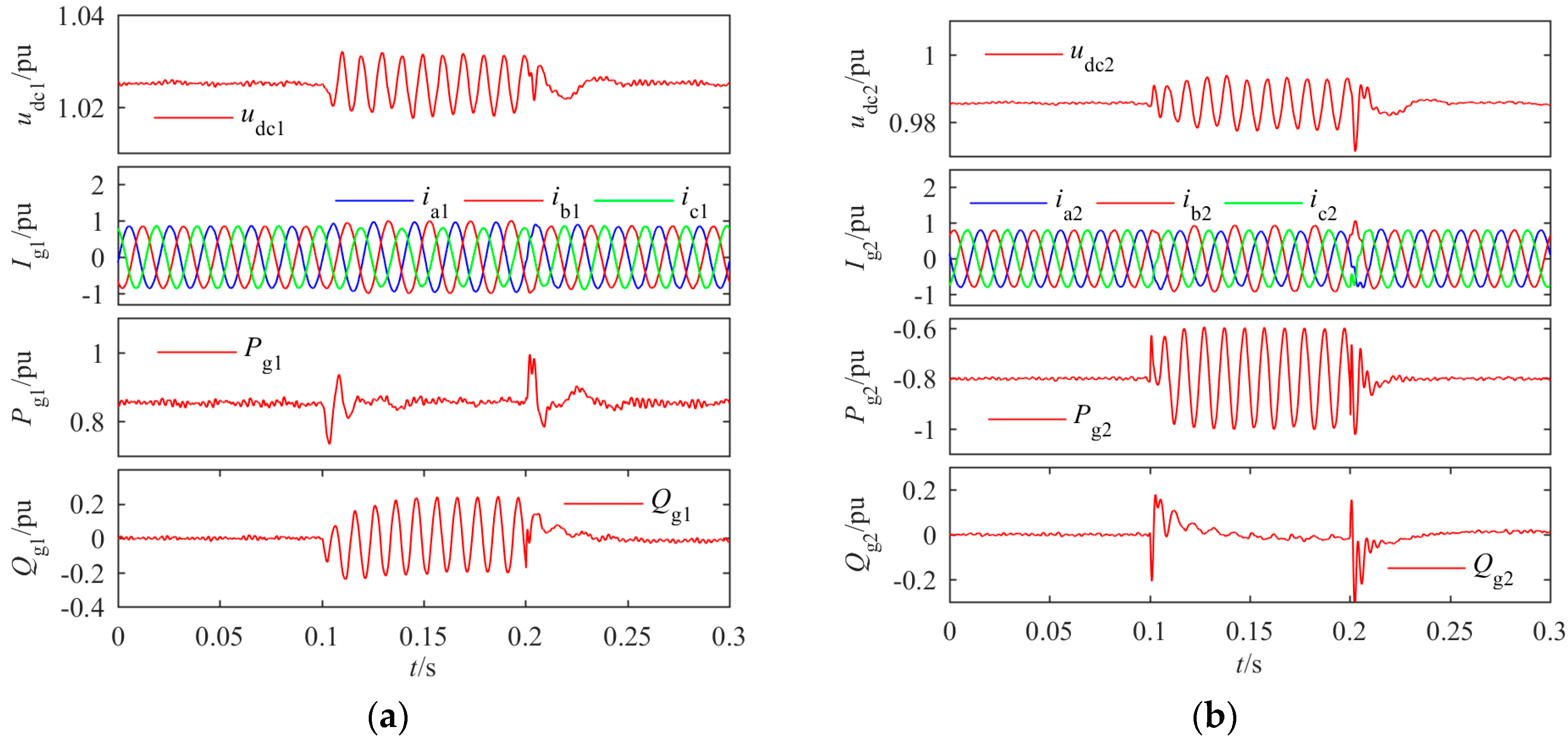
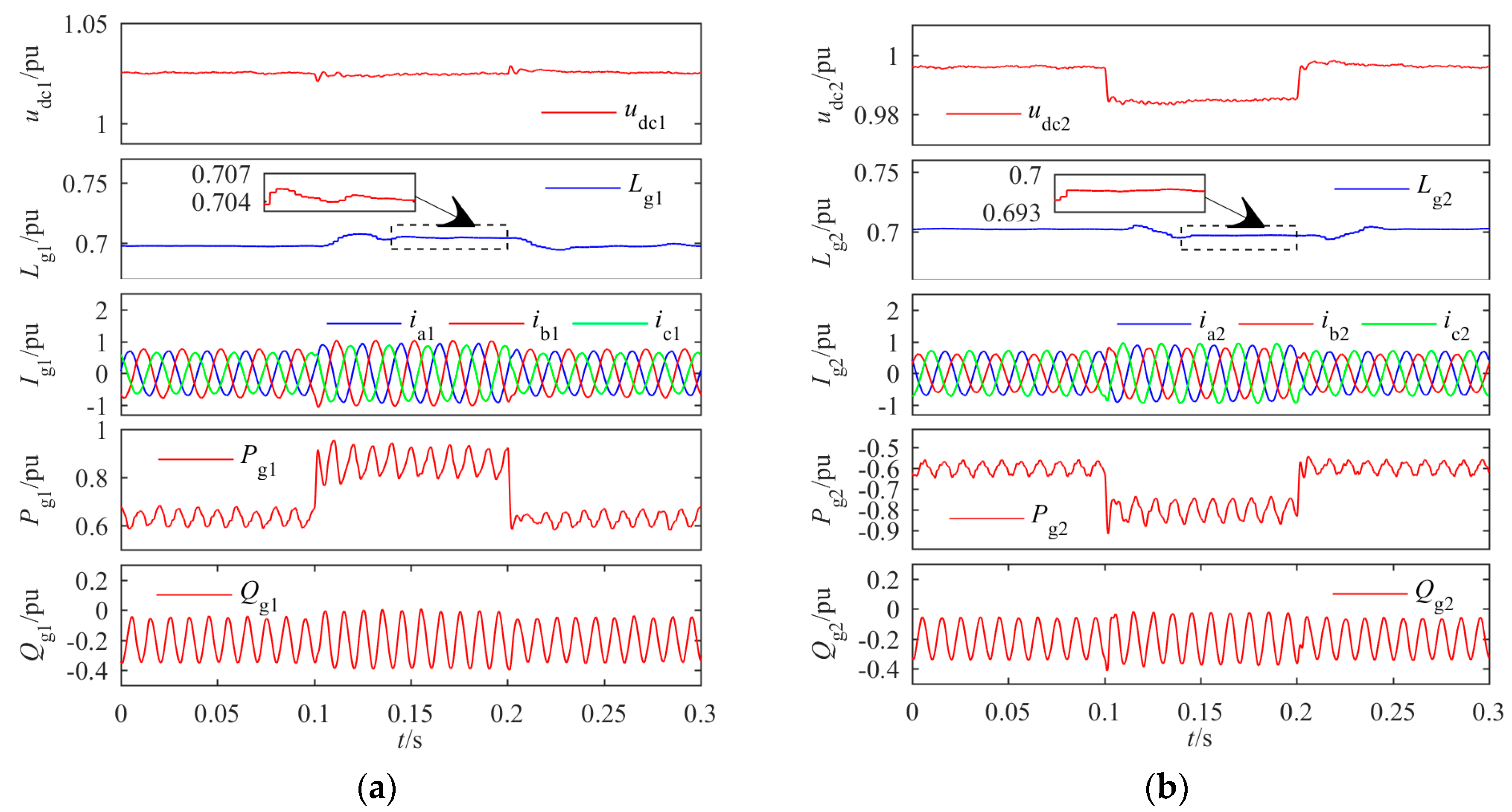
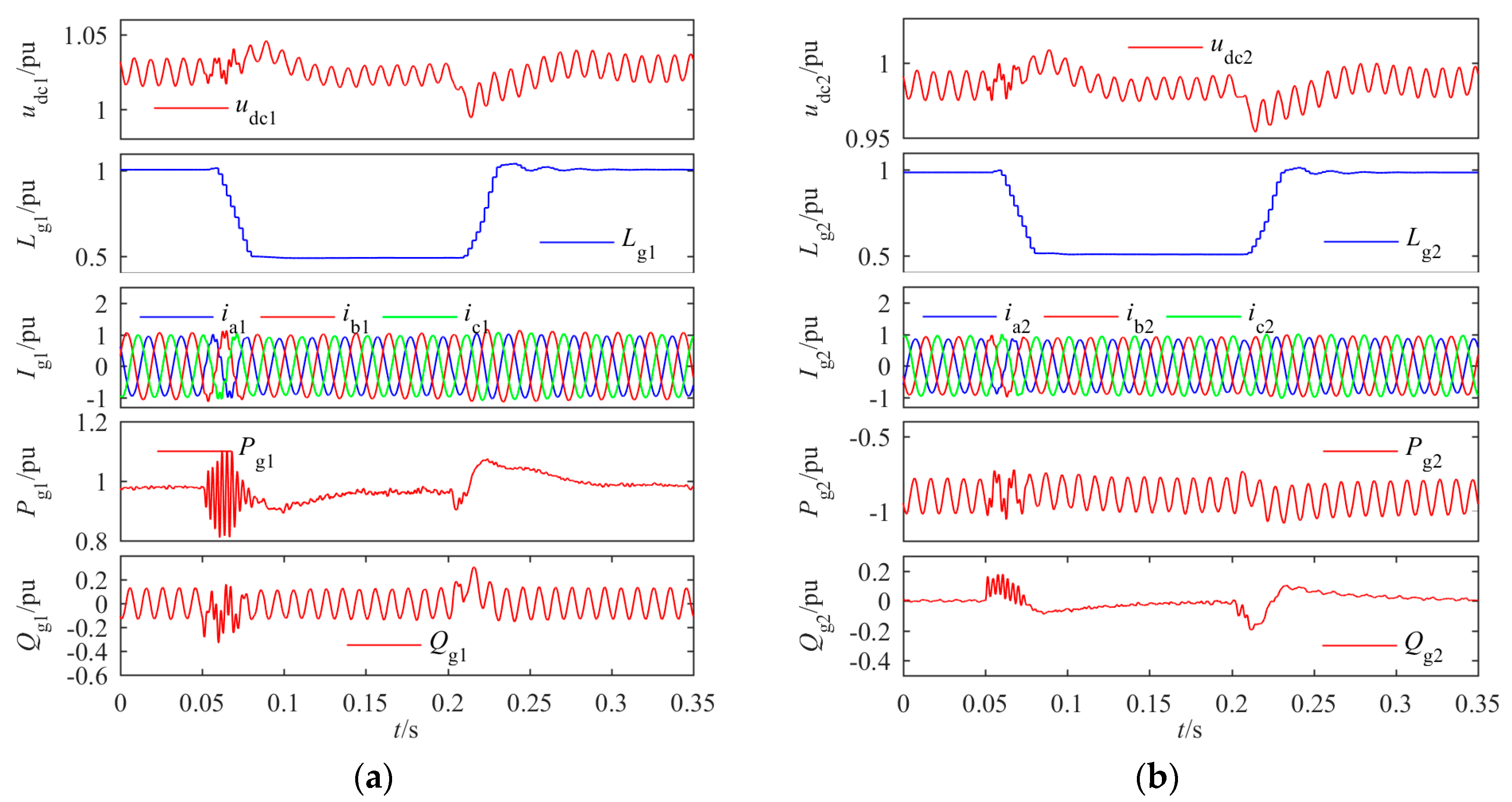
4.2. Simulation Results

For convenience, define the following specified operating condition (SOC), under which most of the simulation studies are conducted. Initially, the grid voltage is three-phase balanced. At 0.1 s, single-phase to ground faults happen to phase A of AC bus B₁ and phase C of AC bus B₂. At 0.2 s, both the faults are cleared and the grid voltages restore to the initial states. The voltage waveforms at PCC1 and PCC2 are as shown in Figure 7. Besides, the inductance of the AC inductors for both CS are set to 75% of the nominal values if not otherwise specified, to investigate robustness of the system.

In Figure 8 the responses of CS1 and CS2 to the SOC for OBJ 1 and OBJ 2 respectively are shown.

From Figure 8 we can see the active power ripples at PCC1 and the reactive power ripples at PCC2 are fully eliminated without current distortion, with the PIDR-SMCC controller. Moreover, the transient performances for both CS are satisfactory. In Figure 9, responses of CS1 and CS2 to the SOC for the control objectives of OBJ 5 are shown. For CS1, $k_{\mathrm{sk}}=0.5$; for CS2, $k_{\mathrm{sk}}=-0.5$.

From Figure 9 we can see the expected control objectives are achieved with the combined function of the GCRC method and the PIDR-SMCC controller. The OAR for CS1 is about 1/3 and that for CS2 is about 3, which is consistent with the theoretical analysis. Figure 10 shows the responses of CS1 and CS2 to the SOC with PIVR controller and PIR controller, respectively. The inductances of the AC inductors for both CS are the nominal values, the control objectives are the same as those in Figure 8. The proportional and integral gains of the two controllers are 1500 and 30,000 respectively. The resonant gains are 18,000 for the PIR controller and 40 for the PIVR controller.

We can see from Figure 10 the steady state performances of both CS are satisfactory with the PIVR and PIR controllers, respectively. However, these are obtained by high controller gains, which will reduce the stability margins. To investigate robustness of the two controllers, responses of CS1 and CS2 to the SOC with reduced AC inductances are shown in Figure 11. In this figure, the grid voltage conditions and the control objectives are the same as those for Figure 10 and the inductances of the AC inductors are set to 80% of the nominal values for both CS.

From Figure 11a we can see that the performances of both CS get worse when the inductances of the AC inductors are reduced by 20%. This is because the reduction of the inductances is equivalent to increase of the control gains. As a result, the system is approaching the stability boundary as the inductance decreases. In Figure 12, the responses of CS1 and CS2 to the SOC with the function of the PIDR-SMCC-OIE controller are shown. The inductances of the AC inductors are 0.7 p.u for both CS, and the control objectives for CS1 and CS2 are to eliminate the active power ripples at PCC1 and to obtain balanced three-phase currents, respectively.

From Figure 12 we can see both the transient and steady state performances of CS1 and CS2 are satisfactory with the PIDR-SMCC-OIE controller, and the inductance estimation results converge to the true values under both balanced and unbalanced grid voltage conditions. In Figure 13, responses of CS1 and CS2 to active power step changes and the SOC under UBGV conditions are shown. The initial average active power demand for CS2 is −0.6 p.u. At 0.1 s, this figure steps up to −0.8 p.u and then stepped back to −0.6 p.u at 0.2 s. The inductances of the AC inductors are 0.7 p.u and the control objectives are to eliminate the DC bus voltage ripples, for both CS.

From Figure 13 we can see that the DC bus voltage ripples on both sides are fully eliminated. The inductance estimation results deviate from the true values for both CS, during the power step-up. However, they are still accurate with relative errors no greater than ±1%. In Figure 14, the responses of both CS to inductance parameter step changes under UBGV conditions are shown to investigate the tracking performance of the OIE.

In this case, the grid voltages are the same as those in Figure 13 and the control objectives are the same as those in Figure 8, for both CS. Initially, the inductances of the AC inductors are 1.0 p.u; at 0.05 s, they are stepped to 0.5 p.u and then stepped back to 1.0 p.u at 0.2 s.

We can see from Figure 14 that the OIE tracks rapidly and accurately the inductance changes all through the process. As a result, the steady state performances of CS1 and CS2 are satisfactory with the PIDR-SMCC-OIE controller even in the presence of the combined effects of voltage disturbances and inductance parameter step changes, although it takes longer time for both CS to settle down.

5. Conclusions

In this paper, a PIDR law-based sliding mode current control strategy with online inductance estimator (i.e., the PIDR-SMCC-OIE strategy) is presented for VSC-MVDC system converter station, under unbalanced grid voltage conditions. The main conclusions are as the following. First, through adding a slack coefficient to the conventional current reference calculation equations, the ratio of the active power ripple amplitude to that of the reactive power ripple can be continuously controlled without current distortion. Second, adoption of the SMC method simplifies the controller design and guarantees closed-loop stability of the system in the Lyapunov sense in the presence of parameter uncertainty and disturbance. Moreover, derivatives of the current references are obtained by simple algebraic operations, which facilitate the implementation of the controller. Third, the OIE presented is easy to implement with no additional sensors needed, and it can provide accurate estimates under both balanced and unbalanced grid voltage conditions. Fourth, application of the Barbalat′s lemma and the reduction to absurdity method proves convergence of the current control errors to zero. Theoretical analysis and simulation studies in PSCAD/EMTDC verify the effectiveness and superiority of the proposed PIDR-SMCC-OIE strategy.

References

1. Wang, Y.; Song, Q.; Zhao, B.; Li, J.; Sun, Q.; Liu, W. Quasi-square-wave modulation of modular multilevel high-frequency DC converter for medium-voltage DC distribution application. IEEE Trans. Power Electron. 2017, 33, 7480–7495. [Google Scholar] [CrossRef]
2. Cairoli, P.; Dougal, R.A. Fault detection and isolation in medium-voltage DC microgrids: Coordination between supply power converters and bus contactors. IEEE Trans. Power Electron. 2018, 33, 4535–4546. [Google Scholar] [CrossRef]
3. Zeng, Y.; Zou, G.; Wei, X.; Sun, C.; Jiang, L. A novel protection and location scheme for pole-to-pole fault in MMC-MVDC distribution grid. Energies 2018, 11, 2076. [Google Scholar] [CrossRef]
4. Yang, W.; Zhang, A.; Zhang, H.; Wang, J.; Li, G. Adaptive integral sliding mode direct power control for VSC-MVDC system converter stations. Int. Trans. Electr. Energy Syst. 2018, 28, e2516. [Google Scholar] [CrossRef]
5. Che, Y.; Li, W.; Li, X.; Zhou, J.; Li, S.; Xi, X. An Improved coordinated control strategy for PV system integration with VSC-MVDC technology. Energies 2017, 10, 1670. [Google Scholar] [CrossRef]
6. Sun, D.; Wang, X.; Nian, H.; Zhu, Z.Q. A sliding-mode direct power control strategy for DFIG under both balanced and unbalanced grid conditions using extended active power. IEEE Trans. Power Electron. 2018, 33, 1313–1322. [Google Scholar] [CrossRef]
7. Jia, J.; Yang, G.; Nielsen, A. Fault analysis method considering dual-sequence current control of VSCs under unbalanced faults. Energies 2018, 11, 1660. [Google Scholar] [CrossRef]
8. Leon, A.E.; Mauricio, J.M.; Solsona, J.A.; Gomez-Exposito, A. Adaptive control strategy for VSC-based systems under unbalanced network conditions. IEEE Trans. Smart Grid 2010, 1, 311–319. [Google Scholar] [CrossRef]
9. Moharana, A.; Dash, P.K. Input-output linearization and robust sliding-mode controller for the VSC-HVDC transmission link. IEEE Trans. Power Deliv. 2010, 25, 1952–1961. [Google Scholar] [CrossRef]
10. Song, H.-S.; Nam, K. Dual current control scheme for PWM converter under unbalanced input voltage conditions. IEEE Trans. Ind. Electron. 1999, 46, 953–959. [Google Scholar] [CrossRef]
11. Hu, J.; He, Y.; Xu, L.; Williams, B.W. Improved control of DFIG systems during network unbalance using PI–R current regulators. IEEE Trans. Ind. Electron. 2009, 56, 439–451. [Google Scholar] [CrossRef]
12. Zhang, J.; Zhao, C. Control strategy of MMC-HVDC under unbalanced grid voltage conditions. J. Power Electron. 2015, 6, 1499–1507. [Google Scholar] [CrossRef]
13. Sun, L.X.; Chen, Y.; Wang, Z.; Ju, P. Optimal control strategy of voltage source converter-based high-voltage direct current under unbalanced grid voltage conditions. IET Gener. Transm. Distrib. 2016, 10, 444–451. [Google Scholar] [CrossRef]
14. Wang, Z.; Zhang, A.; Zhang, H.; Ren, Z. Control strategy for modular multilevel converters with redundant sub-modules using energy reallocation. IEEE Trans. Power Deliv. 2017, 32, 1556–1564. [Google Scholar] [CrossRef]
15. Nian, H.; Song, Y. DFIG operation control strategy under distorted grid conditions based on VPI current regulators. Proc. CSEE 2013, 33, 101–111. [Google Scholar]
16. Liang, Y.; Liu, J.; Zhang, T.; Yang, Q. Arm current control strategy for MMC-HVDC under unbalanced conditions. IEEE Trans. Power Deliv. 2017, 32, 125–134. [Google Scholar] [CrossRef]
17. Teodorescu, R.; Blaabjerg, F.; Liserre, M.; Loh, P.C. Proportional-resonant controllers and filters for grid-connected voltage-source converters. IEE Proc. Electr. Power Appl. 2006, 153, 750–762. [Google Scholar] [CrossRef]
18. Mehrasa, M.; Godina, R.; Pouresmaeil, E.; Vechiu, I.; Rodriguez, R.L.; Catalao, J.P.S. Synchronous Active Proportional Resonant-Based Control Technique for High Penetration of Distributed Generation Units into Power Grids. In Proceedings of the IEEE PES Innovative Smart Grid Technologies Conference Europe, Torino, Italy, 26–29 September 2017. [Google Scholar]
19. Jiang, W.; Ma, W.; Wang, J.; Wang, L.; Gao, Y. Deadbeat control based on current predictive calibration for grid-connected converter under unbalanced grid voltage. IEEE Trans. Ind. Electron. 2017, 64, 5479–5491. [Google Scholar] [CrossRef]
20. Vazquez, S.; Leon, J.I.; Franquelo, L.G.; Rodriguez, J. Model predictive control: A review of its applications in power electronics. IEEE Ind. Electron. Mag. 2014, 8, 16–31. [Google Scholar] [CrossRef] [Green Version]
21. Jiang, W.; Ding, X.; Ni, Y.; Wang, J.; Wang, L.; Ma, W. An improved deadbeat control for a three-phase three-line active power filter with current-tracking error compensation. IEEE Trans. Power Electron. 2018, 33, 2061–2072. [Google Scholar] [CrossRef]
22. Young, H.A.; Perez, M.A.; Rodriguez, J. Analysis of finite-control-set model predictive current control with model parameter mismatch in a three-phase inverter. IEEE Trans. Ind. Electron. 2016, 63, 3100–3107. [Google Scholar] [CrossRef]
23. Mehrasa, M.; Adabi, M.E.; Pouresmaeil, E.; Adabi, J.; Bo, N.J. Direct Lyapunov control (DLC) technique for distributed generation (DG) technology. Electr. Eng. 2014, 96, 309–321. [Google Scholar] [CrossRef]
24. Kordkheili, H.H.; Banejad, M.; Kalat, A.A.; Pouresmaeil, E.; Catalão, J.P.S.; Sciubba, E. Direct-Lyapunov-based control scheme for voltage regulation in a three-phase islanded microgrid with renewable energy sources. Energies 2018, 11, 1161. [Google Scholar] [CrossRef]
25. Pahlevaninezhad, M.; Das, P.; Drobnik, J.; Jain, P.K.; Bakhshai, A. A new control approach based on the differential flatness theory for an ac/dc converter used in electric vehicles. IEEE Trans. Power Electron. 2012, 27, 2085–2103. [Google Scholar] [CrossRef]
26. Mehrasa, M.; Pouresmaeil, E.; Taheri, S.; Vechiu, I.; Catalão, J.P.S. Novel control strategy for modular multilevel converters based on differential flatness theory. IEEE J. Emerg. Sel. Top. Power Electron. 2018, 6, 888–897. [Google Scholar] [CrossRef]
27. Fan, X.; Guan, L.; Xia, C.; Ji, T. IDA-PB control design for VSC-HVDC transmission based on PCHD model. Int. Trans. Electr. Energy Syst. 2015, 25, 2133–2143. [Google Scholar] [CrossRef]
28. Mehrasa, M.; Rezanejhad, M.; Pouresmaeil, E.; Catalão, J.P.S.; Zabihi, S. Analysis and Control of Single-Phase Converters for Integration of Small-Scaled Renewable Energy Sources into the Power Grid. In Proceedings of the 7th Power Electronics, Drive Systems & Technologies Conference (PEDSTC), Tehran, Iran, 16–18 February 2016. [Google Scholar]
29. Shang, L.; Hu, J. Sliding-mode-based direct power control of grid-connected wind-turbine- driven doubly fed induction generators under unbalanced grid voltage conditions. IEEE Trans. Energy Convers. 2012, 27, 362–373. [Google Scholar] [CrossRef]
30. Gong, H.; Wang, Y.; Li, Y.; Li, X.; Wei, L. An input-output feedback linearized sliding mode control for D-STATCOM. Autom. Electr. Power Syst. 2016, 40, 102–108. [Google Scholar]
31. Yang, W.; Zhang, A.; Li, J.; Li, G.; Zhang, H.; Wang, J. Integral plus resonant sliding mode direct power control for VSC-HVDC systems under unbalanced grid voltage conditions. Energies 2017, 10, 1528. [Google Scholar] [CrossRef]
32. Mehrasa, M.; Hosseini, S.K.; Taheri, S.; Pouresmaeil, E.; Catalão, J.P.S. Dynamic Performance Control of Modular Multilevel Converters in HVDC Transmission Systems. In Proceedings of the IEEE Electrical Power and Energy Conference, Ottawa, ON, Canada, 12–14 October 2016. [Google Scholar]
33. Mahdian-Dehkordi, N.; Namvar, M.; Karimi, H.; Piya, P.; Karimi-Ghartemani, M. Nonlinear adaptive control of grid-connected three-phase inverters for renewable energy applications. Int. J. Control 2017, 90, 53–67. [Google Scholar] [CrossRef]
34. Xia, C.; Wang, M.; Song, Z.; Liu, T. Robust model predictive current control of three-phase voltage source PWM rectifier with online disturbance observation. IEEE Trans. Ind. Inform. 2012, 8, 459–471. [Google Scholar] [CrossRef]
35. Chen, C.; Li, L.; Zhang, Q.; Tong, Q.; Liu, K.; Lyu, D.; Min, R. Online inductor parameters identification by small-signal injection for sensorless predictive current controlled boost converter. IEEE Trans. Ind. Inform. 2017, 13, 1554–1564. [Google Scholar] [CrossRef]
36. Kabiri, R.; Holmes, D.G.; McGrath, B.P. Control of active and reactive power ripple to mitigate unbalanced grid voltages. IEEE Trans. Ind. Appl. 2016, 52, 1660–1668. [Google Scholar] [CrossRef]
37. Wang, Y.; Ou, M.; Chen, Y.; Chen, Z.; Xiao, Z.; Xu, Z.; Wang, Y. Coordinate control of power fluctuation suppression and current balance under unbalanced voltage conditions. Proc. CSEE 2017, 37, 6981–6987. [Google Scholar]
38. Anderson, B. Exponential stability of linear equations arising in adaptive identification. IEEE Trans. Autom. Control 1977, 22, 83–88. [Google Scholar] [CrossRef]
39. Slotine, J.-J.E.; Li, W. Applied Nonlinear Control; China Machine Press: Beijing, China, 2006; pp. 365–366. ISBN 7-111-18379-7. [Google Scholar]
Figure 1. Single-line diagram of the two-terminal voltage source converter medium voltage direct current (VSC-MVDC) system studied.
Energies 11 02599 g001
Figure 2. Schematic of three-phase VSC for each converter station.
Energies 11 02599 g002
Figure 3. Space vector of the gird voltage in the positive sequence (PS) and negative sequence (NS) synchronous reference frame (SRF).
Energies 11 02599 g003
Figure 4. An example to show the relationships between Pgsin2, Pgcos2, Qgsin2, Qgcos2 and ksk.
Energies 11 02599 g004
Figure 5. Schematic of VSC system with ideal switch.
Energies 11 02599 g005
Figure 6. Block diagram of the proportional-integral-derivative-resonant law-based sliding mode current control strategy with online inductance estimator (PIDR-SMCC-OIE).
Energies 11 02599 g006
Figure 7. The grid voltage waveforms of the specified operating condition (SOC) for CS1 (a) and CS2 (b).
Energies 11 02599 g007
Figure 8. Responses of CS1 (a) and CS2 (b) to the SOC for OBJ 1 and OBJ 2 respectively.
Energies 11 02599 g008
Figure 9. Responses of CS1 (a) and CS2 (b) to the SOC for OBJ 5.
Energies 11 02599 g009
Figure 10. Responses of CS1 (a) and CS2 (b) to the SOC with proportional-integral plus vector resonant (PIVR) and proportional-integral plus resonant (PIR) controllers respectively.
Energies 11 02599 g010
Figure 11. Responses of CS1 (a) and CS2 (b) to the SOC by the PIVR and PIR controllers with 20% reduced inductances respectively.
Energies 11 02599 g011
Figure 12. Responses of CS1 (a) and CS2 (b) to the SOC with the function of the PIDR-SMCC-OIE controller for OBJ 1 and OBJ 3 respectively.
Energies 11 02599 g012
Figure 13. Responses of CS1 (a) and CS2 (b) to active power step changes under unbalanced grid voltage (UBGV) conditions for obtaining constant DC bus voltage.
Energies 11 02599 g013
Figure 14. Responses of CS1 (a) and CS2 (b) to inductance parameter step changes under UBGV conditions.
Energies 11 02599 g014