Article

An Improved Fuzzy C-Means Algorithm for the Implementation of Demand Side Management Measures

1
Department of Electrical Engineering, Western Macedonia University of Applied Sciences, Kozani 50100, Greece
2
Department of Electrical Engineering, Technological Educational Institute of Thessaly, Larisa 41110, Greece
3
Energy and Environmental Policy Laboratory, School of Economics, Business and International Studies, University of Piraeus, Piraeus 18532, Greece
*
Authors to whom correspondence should be addressed.
Energies 2017, 10(9), 1407; https://doi.org/10.3390/en10091407
Submission received: 6 August 2017 / Revised: 4 September 2017 / Accepted: 12 September 2017 / Published: 14 September 2017
(This article belongs to the Section F: Electrical Engineering)

Abstract

:
Load profiling refers to a procedure that leads to the formulation of daily load curves and consumer classes regarding the similarity of the curve shapes. This procedure incorporates a set of unsupervised machine learning algorithms. While many crisp clustering algorithms have been proposed for grouping load curves into clusters, only one soft clustering algorithm is utilized for the aforementioned purpose, namely the Fuzzy C-Means (FCM) algorithm. Since the benefits of soft clustering are demonstrated in a variety of applications, the potential of introducing a novel modification of the FCM in the electricity consumer clustering process is examined. Additionally, this paper proposes a novel Demand Side Management (DSM) strategy for load management of consumers that are eligible for the implementation of Real-Time Pricing (RTP) schemes. The DSM strategy is formulated as a constrained optimization problem that can be easily solved and therefore, making it a useful tool for retailers’ decision-making framework in competitive electricity markets.

1. Introduction

In order to cope with the rapidly increasing energy demand in many countries, modern electric power system planning relies on two fundamental concepts, namely Supply Side Management (SSM) and Demand Side Management (DSM) [1]. In the first case, the demand increment is dealt with by power capacity expansion. The required time period for the installation of centralized power plants that will cover the electricity needs is large. Moreover, the continuous utilization of fossil fuels in the power generation and transport sectors gives rise to environmental concerns. Many countries have set minimum requirements regarding the generation capacity expansion planning in order to meet specific environmental protection targets. In addition, many electricity generation schemes such as Renewable Energy Sources (RES) depend on unforeseen parameters like the weather conditions. The intermittent power generation of certain types of RES, though, yields problems in the reliability and balance of the grid. Also, high RES penetration in the grid results in increased needs of operational reserves, investments in transmission and distribution infrastructure, and sophisticated methods of solar and aeolic capacity forecasts. On the other hand, DSM seeks methods to modify the demand patterns for a variety of purposes such as lowering the risks that accompany high demand peaks, generation shortages and transmission network congestion [2].
DSM is a basic tool of the Smart Grid [3,4,5,6,7,8,9]. It is a fact that modern system planning focuses on the gradual transition to the Smart Grid, which is based on advanced distributed information systems. The Smart Grid coordinates the needs and the resources of utilities, grid operators, consumers and other market entities, in a way that all electricity grid components would function in the optimal manner, simultaneously minimizing the costs and influence on the environment, and maximizing the stability, reliability and adaptability of the grid. Smart Grids incorporate advanced metering infrastructure together with the accompanying communication technologies, in order to record, collect and store load data and to apply measures that will influence the demand patterns [10,11,12].
Moreover, DSM plays a significant role in the operation of energy markets. As a pillar of DSM, Demand Response (DR) aims to modify demand through incentive and price-based programs. Price-based DR includes dynamic pricing schemes such as Time-Of-Use (TOU) rates, Critical Peak Pricing (CPP), Real-Time Pricing (RTP) and others [13,14,15]. In particular RTP is considered as an efficient mechanism for transferring the actual generation costs to the end-consumers [16]. Following a RTP program, the consumer can take advantage of low prices during specific periods and lower his consumption [17].
Through DR programs, the consumer plays a more active role in the energy market. Many research efforts and pilot programs have been presented so far for the assessment of the barriers and benefits of DR programs [18]. In most studies, the DR program is investigated as a concept to increase the revenues of a load serving entity (i.e., the Retailer). The overall scope is to seek how the tariff should be formulated in order to maximize the Retailer’s benefits [19]. No emphasis on achieving a DSM target is placed. Hence, the tariff structure found in a DR program is centered on maximizing the profits of the Retailer in the market. In the present paper, a different approach is followed. The tariff structure is built upon the requirements of a DSM target that is decided prior to the day that is asked to be delivered. In order to achieve a pre-defined DSM target via price-based DR programs such as RTP, the present paper proposes an optimization model. The decision variables of the model are the hourly prices that need to be extracted in order to simultaneously satisfy the DSM target and place the Retailer within market competition. One way to achieve the latter is to set price limits. The main objective of the paper is to propose a model that relates DSM and DR in a coherent way. Overall, the objectives of the paper are:
  • The present paper aims to fully connect the DSM targets with price-based DR. The latter is widely regarded in the literature as an efficient mechanism to alter the demand patterns of the consumers. The model developed in the paper outputs tariffs that emphasize on achieving a pre-defined DSM objective. Therefore, the benefits of RTP are evident in power grid scale and not restricted to the load serving entity.
  • The flexibility of the consumer to alter the demand according to the tariff is expressed by the elasticity. This parameter is part of the model’s operation. A novel technique is proposed to derive dynamic elasticities that more accurately capture the changes in the demand according to tariffs.
  • A part of the model’s operation is the utilization of unsupervised machine learning techniques such as soft clustering for a two-fold purpose: (a) to extract the representative load curves or load profiles of the consumers and (b) to track similarities in historical loads for the purpose of drawing the dynamic elasticities curves.
The model can be applied in intra-days energy markets and there is no restriction on the number of consumers or on the type of the involved DR program.

2. Literature Review and Method

This section provides a review of the state of the art concerning DSM techniques and methodologies, DR programs, RTP schemes, and clustering methods, which illustrate the contributions of this work. This is followed by a description of the methodological approach and the assumptions used in this work.

2.1. State of the Art

The DSM term includes a variety of approaches and technologies. Whereas the benefits of DSM are discussed in many studies [20,21], the implementation of a DSM program needs to address various issues such as data collection, consumer behaviour, appropriate control strategies and others [22]. RTP has gathered the attention of many researchers that have approached it from different perspectives, such as peak capacity reduction, electricity bill savings, wholesale market price reduction, renewables utilization and others [16]. The majority of the RTP literature focuses on residential consumers. This is due to the fact that the availability of load data of this consumer category is high. There are generally two options for applying the RTP in the residential sector: (a) as price signals sent by the Retailer [23] and (b) as part of the operation of home energy management systems [24]. Although many studies have focused on the residential consumers [25], industrial DSM examples are few. According to [26], the potential of DSM in industries is high due to the facts that: (a) the individual power consumption is very high, a fact that motivates and eases participation in DSM programs; (b) the capital investment required for DSM is zero since the metering infrastructure is already installed; and (c) industrial processes are operated in isolated environments leading to low or even no requirements for human comfort. However, many issues arise in industrial environments that need to be regarded in the design steps of a DSM program [27]. Any assessment of industrial processes apart from electricity usage tasks, has to consider the use of multiple resources such as raw materials. This fact raises limitations on the simultaneous management of energy and resources. Furthermore, many industrial facilities are complex and their modeling becomes difficult. There is, also, a lack of energy management approaches for real-time DSM. In [27], the objective is to minimize the production cost while satisfying the production target. The future real-time prices are forecasted with an appropriate neural network. In [28], the goal is to minimize the operating costs of an industry according to hourly fluctuations of electricity prices in a 1 week-ahead period. The optimization problem seeks to define production levels, modes of operation, inventory levels and product sales on an hourly basis. In [29], a DR energy management scheme for industrial facilities is proposed. The scheme divides the processing tasks in industrial facilities into non-schedulable and schedulable tasks and takes advantage of distributed energy resources to implement DR. The day-ahead electricity prices are taken into account in order to optimally schedule the schedulable tasks and the distributed energy resources. The scope is to shift demand from peak to off-peak periods. In [30], the problem of determining an operations plan that minimizes the cost of running an air separation plant under RTP is discussed. The authors define the conditions under which RTP is the most attractive pricing scheme for a production facility in the industrial gas industry. In [31], a real-time decision framework for the load management of an industrial manufacturing process is proposed. The authors argue that inherent dependence between consecutive tasks in a manufacturing process are present. In the view of this fact, the proposed model takes future load management into consideration. The case study was conducted on a steel powder manufacturing process. In [32], the objective function refers to the minimization of electricity cost. The authors examine four different cases of contracts: (a) hourly volatile prices with peaks; (b) fixed prices; (c) TOU rates and (d) hourly volatile prices without peaks. The conclusions of the paper state that cost reduction is higher in the case of hourly varying prices compared with TOU rates and fixed prices. A peak load shifting DR-based strategy is examined in [33]. The developed model includes task scheduling of four processes in an industrial refinery plant. In [34], the authors propose a multi-battery optimal scheduling program subject to RTP. The objective is to minimize the production cost in terms of lowering the electricity bills.
Price-based DR programs have been approached in the literature in terms of profit maximization in deregulated energy markets. The related entity in the market for DR is the Retailer that acts as the intermediate agent between generation companies and consumers. Subject to expenses that are related to the procurement of electricity, the target of DR is to maximize the profits through efficient pricing schemes [35,36]. The price offered to consumers can be constant or variable, i.e., different prices are applied per hour. Most studies in Retailer profit problems focus on the optimal procurement mechanism, i.e., forward contracts, call options, pool market and self-production [37,38,39,40,41]. Another factor that indirectly influences profits, due to the risks of power market prices, is the prediction of these prices. In [37,38,39,40,41] market prices are forecasted using time series models such as ARIMA. However, more reliable forecasting models have been proposed in the literature [42,43].
The decisions of the Retailer are categorized as long or short-term. Dynamic pricing is considered in [19,23,41] focusing on the tariffs. Apart from the costs that are related with the procurement mechanism, a crucial parameter is the DR of the consumers. RTP is considered in [19], where different price/demand functions are examined in order to evaluate the influence of the type of the aforementioned function in the profits. In [23], the test set includes 300 consumers connected in the 20 kV distribution network in Iran. The consumers are clustered into four clusters and for each cluster a different RTP profile is applied. The procurement mechanism corresponds to the pool market. No method is used for risk modeling and management. In [35], the scope is to define the optimal procurement mechanism. The mechanisms considered are spot price, forward contracts, call option and self-production. Future market prices and consumer load are considered as stochastic variables. The exposure of the Retailer in the uncertainties of future spot prices is modeled with the conditional-value at risk parameter. The results indicate that the risk parameters affect the offered price to the consumer. More specifically, if the Retailer tends to be risky, i.e., to rely for its procurement on the spot market, the offered price is higher. In [36], the Retailer serves five different consumers. The electricity is purchased from the pool market. The authors include a wide set of scenarios in their analysis that differ in terms of price strategy (i.e., flat and TOU rates), maximum price limit, and elasticity value. The authors conclude that the optimal price strategy, i.e., the one that leads to higher profits, is TOU rates. Also, as the consumers become more elastic, the profits of the Retailer decline. The authors of [37] focus on the PJM energy market. As in [35], market prices and load are treated as stochastic variables and various scenarios are generated. These two factors influence Retailer profits and a careful simulation of them appears to be crucial in profit maximization. In [38], the scope is to address the contract design both at the supply and end-user levels. The paper provides a stochastic programming methodology that allows the Retailer to make informed contractual decisions, particularly in respect to contract prices and quantities. A stochastic-based optimization model is proposed in [39]. The Retailer’s decisions are distinguished in short- and medium-term based on the procurement mechanism involved, i.e., pool market and forward contract. The Retailer serves a residential, a commercial and an industrial consumer. The authors focus on the influences of the type of the procurement mechanism and the risk parameter value on the profits. The work in [39] is expanded in [40]. The consumers’ reaction to the offered price is modeled with a linear price/demand function. The methodology of [23] is enriched in [41]. In this paper, the approach of the Retailer towards the risks associated with the pool market is modeled with the conditional value at risk method. The response of the consumers to the offered price by the Retailer is modeled by a piece-wise acceptance function. This function relates the number of consumers that accept a specific price value.
A model between price and responsive demand requires a mathematical formula, known as price/demand function [44]. The price/demand function indicates how a change in price affects the load. The flexibility of the demand to the offered price by the Retailer is expressed by the price elasticity parameter [45]. In the majority of the related studies in the literature, the elasticity is considered constant within the 24 h period or receives different values per period, namely off-peak and peak hours. As defined in profit maximization literature, the elasticity only relates to load and price, namely it represents the price elasticity. No other factors that influence demand are taken into account. The values of price elasticities are set out by the analyst or taken by previous econometric studies [37,38]. Moreover, consumers of the same activity, i.e., residential, industrial and others are considered having the same price elasticity value. However, this approach does not always reflect the actual behavior of the consumer.
A detailed knowledge of the demand patterns influence the success of DR programs and has an influence on profits. Load profiling is tested as an approach to derive representative or typical demand patterns [46,47]. The latter refers to the formulation of typical load curves for single consumers and groups of consumers. Based on certain criteria, the consumers are grouped together in a number of clusters. Each cluster has a representative daily load curve, which is the weighted average of the diagrams that belong to the cluster. According to this approach, the consumers are not only distinguished in macro-categories (i.e., residential, commercial, etc.), but sub-categories are formed within the macro-classes. A load profiling problem is formulated as an unsupervised machine learning task and the objective is to optimally classify load with a similar pattern. The algorithms that have been proposed in the load profiling related literature can be distinguished into five general classes: (a) partitional algorithms, such as the K-means and others; (b) hierarchical agglomerative algorithms; (c) fuzzy algorithms, such as the FCM; (d) neural network-based algorithms, such as the Self-Organizing Map (SOM) and Hopfield network; and (e) algorithms that do not belong to the above classes, such as the Renyi Entropy Clustering, Competitive Leaky Algorithm (CLA) and others [46,47,48,49,50,51,52,53,54,55,56,57,58,59,60,61,62,63,64,65,66].
Crisp or hard clustering assigns each pattern to exactly one cluster. Soft clustering is a generalization of crisp clustering. The patterns are assigned to all clusters with partial membership. This leads to flexibility in the definition of the clusters’ configurations. Soft clustering is suitable when the presence of noise or the erroneous representation of the patterns is an obstacle to the clustering outcome. Also, soft clustering is beneficial in cases where the distinctions margins of the generated clusters in the feature space are vague. The advantages of soft clustering have been shown in a wide diversity of research fields [67,68].
FCM has been occupied in load profiling tasks as a sole algorithm [53,55,57,58,59,60,61] or as a part of a comparison among many algorithms [48,50,51,62,63,64,65,66]. In [48], the utilized data set includes 234 non-residential consumers. A comparison between K-means, FCM, Ward hierarchical algorithm, average distance criterion hierarchical algorithm, SOM and modified follow-the-leader algorithm was performed. The algorithm evaluation is done with four validity indicators or adequacy measures. The modified follow-the-leader algorithm wins the competition. The FCM is only superior to the SOM. In [50], the same algorithms as in [48] are used, plus the support vector clustering algorithm. The latter is more effective than the rest. In [51], three algorithms based on the Renyi entropy distance criterion are presented. The authors examine the same data as in [48,50]. In this comparison, FCM is superior to two of the three newly proposed algorithms. In [53], the data set involves 300 load curves coming from distribution feeders in Malaysia that serve domestic, commercial and small size industries consumers. The algorithm’s potency is checked by two validity indicators and the number of output clusters is set to five. The authors of [55] use seven fuzzy validity indicators. An inherent limitation of the fuzzy validity indicators is that they lead in the majority of the cases to small optimal number of clusters. The algorithm is applied to the day load of a city in China curves covering the period of 1 year. The authors argue that the fuzziness index holds an important role in the algorithms operation. The parameter is data specific and several trial-and-error executions should take place in order to calibrate it. The data used in [57] are the same as the test case of [53]. In this paper, the number of clusters is set to four. Since the data refer to aggregate loads coming from feeders, no large differences are observed. As load level increases, the daily load becomes less flexible with a rather deficient shape. After the initial clustering, the FCM is executed again separately in the daily load curves of each cluster. An additional load profile per cluster is drawn leading to the final number of load profile to be equal to eight. In [58], the data set refers to 100 daily load curves obtained from feeders in Malaysia. The FCM is used to cluster the load data. Afterwards, a probabilistic neural network is used to classify the resulting load profiles to pre-defined consumer types. The same authors in [59] focus on the fuzziness parameter. A series of simulations took place in order to define the optimal value. According to the paper’s findings, the parameter increase tends to lead to lower clustering errors. This fact is observed in all validity indicators used in the paper. Gerbec et al. [60] apply the same concept as [58]. The FCM generates the load profiles that are used as part of the training vector of the probabilistic neural network. The other part involves the load profiles of the respective activity types. With this approach, a business activity is allocated into the most probable cluster. In [61], the FCM is applied to 300 low voltage consumers. Next, a feed-forward neural network is used to assign the consumers to the clusters. The inputs of the network are indicators related with monthly energy usage. The outputs correspond to the membership functions of the FCM that refer to the level of certainty with which the assignment of a load curve to a cluster is made. Various combinations with different clusters and different neural network parameters are examined. In [62], a comparison takes place between FCM, K-means and various topologies of the SOM. The authors utilize the Intra Cluster Index (IAI) and the Inter Cluster Index (IEI) validity indicators. The data cover two years and are provided by a utility in Brazil. In [63], the FCM is tested via three validity indicators. The authors conduct an experiment with different values of the fuzziness parameter. As the parameter increases, the clustering errors decrease. Thus, while fuzziness on the formatted clusters tends to decrease, the clustering of a load data set is more robust. In [64], the FCM is compared to hierarchical clustering. No information about the type of hierarchical algorithms is given. Also, the comparison of the algorithms is based on the differences of their theoretical framework. No results are presented regarding the scores of the two algorithms in a validity indicator. The comparison of K-means, FCM and hierarchical algorithm in [65] is based on the shapes of the load profiles that each algorithm results in. The data refer to 288 consumers of the Slovenian distribution grid. The algorithms are applied to the data set and the shapes of the load profiles are discussed. In [66], the comparison includes FCM, spectral clustering and expectation maximization algorithm. The data refer to the total national load of 8 European countries collected by the ENTSO-E database. The authors conclude that spectral clustering appears as the most robust algorithm.
Based on the previous literature survey, the contributions of the present paper are summarized in the following: RTP is utilized not as a part of profit maximization for electricity retailers but as a tool for the implementation of DSM targets. A novel method is proposed to derive time variant price elasticities of consumers’ load. Finally, a novel version of the traditional FCM is proposed for load profiling but also for implementing RTP schemes to meet predefined DSM targets. More specifically:
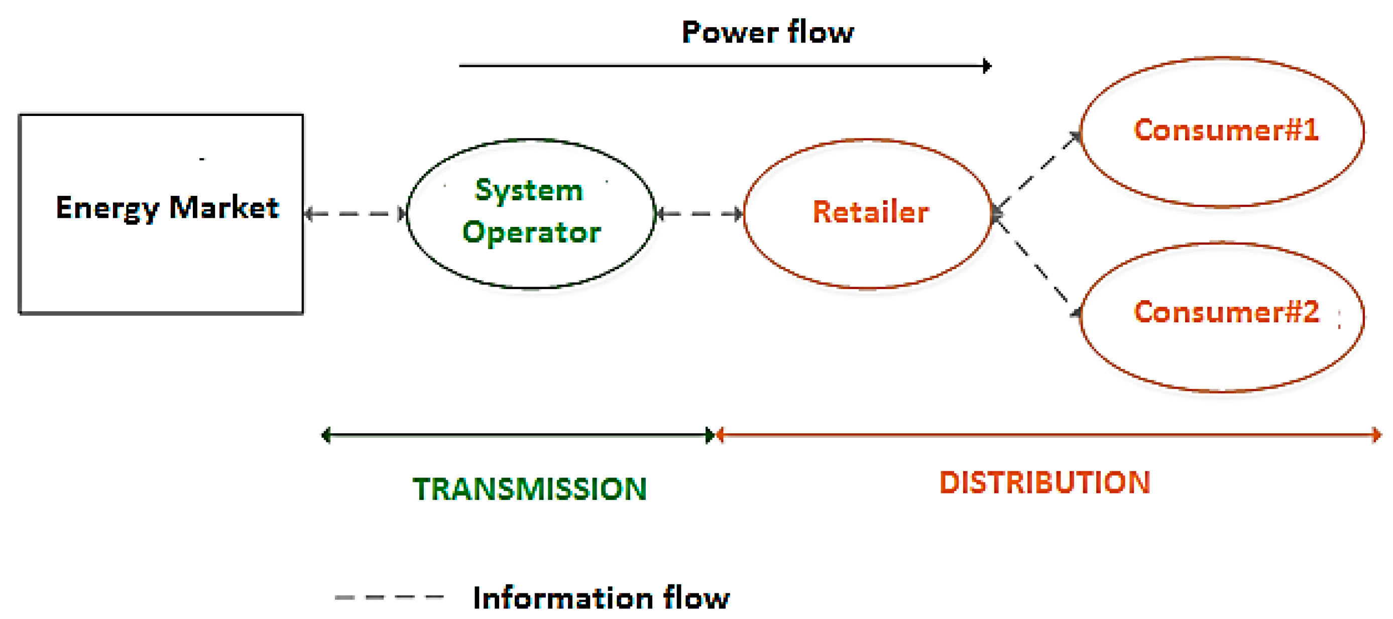
  • In profit maximization problems, no attention is placed on meeting specific goals on shaping the load curves of the consumers. In the present paper, RTP is utilized not as a part of profit maximization for electricity retailers, but as a tool for the implementation of DSM targets. Therefore, price-based DR is used to achieve a load management target. A single case study of a Retailer that interacts with the wholesale market environment and serves the consumers is investigated. For each hour period in an intra-day basis, the Retailer is asked by the System Operator (SO) to deliver specific load modifications refer to as DSM strategy goals, i.e., Peak Clipping, Valley Filling, Load Shifting, Strategic Conservation, Strategic Load Growth and Flexible Load Shape [69,70]. The Retailer implements the appropriate strategy based on the load profiles and the price elasticity of the consumers, market prices and other conditions. The strategy is interpreted as RTP schemes that are transferred to the elastic consumers. The term “elastic” characterizes the consumers that take full advantage the selling price by the Retailer and modify their demand accordingly. Hence, the consumers react to the selling price and achieve the pre-defined DSM objective. The proposed DSM strategy implementation is formed as a single linear constrained optimization task. The decision variables are the prices of the specific hour for the consumers. The price approach of the proposed strategy is consumer oriented; each consumer is offered a specific price profile based on the load profile and price elasticity. This leads to more accurate pricing, not only in terms of transferring the actual generation costs mirrored in the wholesale market, but also in designing consumer-specific tariff products based on the consumer demand patterns.
  • A novel method is proposed to derive time variant price elasticities. The term “dynamic” price elasticity is used to indicate price elasticity curves that express different values per hour. This approach not only represents the actual behavior of the consumer but consumer oriented price elasticities profiles can be drawn.
  • While many crisp algorithms have been proposed in the load profiling literature, the potential of soft clustering has not been adequately demonstrated, since only FCM has been examined. In the present paper, a detailed comparison takes place between two fuzzy algorithms, and their performance is checked by a set of adequacy measures that have been proposed in the load profiling related literature. The goal is to use soft clustering not only for load profiling aims but also to design and implement RTP schemes to meet predefined DSM targets in day-ahead electricity markets.
The analysis of the present paper is concentrated at two High Voltage (HV) industrial consumers located in Greece. The HV industry is considered as energy intensive. Currently, the consumption of HV industries in Greece accounts for 14% of the total consumption of the Greek electric sector [71]. At least theoretically, the potential of implementation of DSM measures to achieve certain DSM goals is high. An ongoing discussion between the Retailers sector and the Regulatory Authority of Energy of Greece, have been taking place regarding the modification of the existing tariffs offered to the HV [72]. This fact raises the need for a more accurate and justified pricing policy.

2.2. Methodological Approach

According to [73], in some cases industrial DSM implementation encounters difficulties due to the nature and operational characteristics of the loads. Although the per process modeling of industrial activity offers a detailed simulation of a DR-based management program, as most authors state, the modeling becomes unfeasible in the case of complex processes. In the present paper, the industrial consumer is examined as a generic block. The consumer itself is responsible for altering the consumption of the electrical or other apparatus as he wishes. It has to be clarified that in the present work the economic benefit and profitability of the Retailer are not examined. The scope is to develop and test a model that outputs the optimal RTP profiles that will fully accomplish a predefined DSM objective. Also, the contribution of each consumer to the objective is derived. The Retailer is not rewarded for delivering the DSM objective asked by the SO. The model’s operation presupposes the existence of a telecommunication infrastructure that enables two-way information flow between the Retailer and consumers. The consumers act rationally and follow the price signals on an hourly basis. No interaction between consumers takes place. The energy market conditions or other factors do not influence the response of the consumers to prices, such as rival Retailers’ contract offers, weather conditions, economic conditions and others. The Retailer’s actions do not influence market prices. The consumers follow the price profiles variations offered by the Retailer with no rights of negotiation. The model outputs automatically the shares of each consumer contributions for achieving the overall DSM target. A test case with two existing industrial consumers within the Greek electric sector is examined. The data sets used for the model refer to the consumption of the consumers and their existing tariffs as offered by their current Retailer.

3. Proposed Model

In the following Sections the model is described. Specifically, the general concept is given in Section 3.1. Next, in Section 3.2 the mathematical description of the DR of the consumers is presented. In this study, three DR models are compared in order to assess the influence of the type of DR modelling in the RTP. In Section 3.3 the DSM objectives are presented and in Section 3.4, the dynamic elasticity extraction method is presented. The mathematical background of load profiling that is described in Section 3.5 includes the pattern representation, the clustering evaluation framework and description of the algorithms.

3.1. Concept

A conceptual diagram of the proposed model is presented in Figure 1. According to market conditions and operational constrains, the SO sends a signal to the Retailer with specific DSM objective on a day-ahead basis. Thus, the DSM objective is known to the Retailer the day ahead that is asked to be manifested. The SO acts in the transmission system and connects the wholesale and retail markets. The Retailer acts in the distribution system level and transfers the commands of the SO to the consumers. Figure 2 depicts the DSM objectives. The figure shows in a simple manner how an initial load curve is affected after the successful exercise of a set of measures that aim at satisfying the objective. The task of the Retailer is to “distribute” the DSM objective to the consumers. For instance, if the SO asks the Retailer for an overall reduction of 1 MW, the Retailer sends different RTP signals to the consumers, specifically designed in order to meet overall the 1 MW target.
In order to demonstrate and assess the proposed model, a single case of a Retailer that serves a number of consumers m = 1, 2, , M with total consumption in day n, P(n, M) is regarded. For each day n the daily load curve of consumer m is expressed as a D-dimension vector x n m = [ x 1 m , , x D m ] T . The dimension of the vector refers to the recorded load time interval of metering. Originally, the two consumers are charged with the same TOUs rates tariffs designed by their current Retailer [71]. These tariffs are referred as “nominal” and indicated as p0(h) at hour h = 1, 2, , 24. Nominal price is a product of bilateral agreement among the Retailer and the consumer. The demand that corresponds to the nominal price p0(h) is referred as “nominal” demand and indicated as d0(h). Based on its load magnitude and price elasticity, every consumer contributes differently in the overall DSM objective. Therefore, it is more accurate for each consumer to be charged with a different RTP scheme. Let p1(h) and p2(h) (€/kWh) be the RTPs at hour h within the day, of the 1st and 2nd consumer, respectively. These prices are accepted by the consumers who modify their loads accordingly, and finally the DSM objective is met. While price-based DR programs such as RTP are voluntary, the consumers are considered elastic, take full advantage of the hourly RTP, and respond rationally. The DR of the consumer d(p(h)) corresponds to price p(h).

3.2. Demand Response Models

3.2.1. Linear Price/Demand Function

In the present study, three price/demand functions are considered for the purpose of examining the influence of the selection of the function on the DSM success. The simplest price/demand function is linear dlin(p(h)) = alin + blinp(h), where alin and blin are two coefficients of the linear function. Let d 0 l i n ( h ) be the nominal demand of the consumer using the linear demand function, and B 0 l i n ( h ) the nominal consumer benefit (€) that corresponds to demand d 0 l i n ( h ) . The obtained benefit Bc(dlin(p(h))) that corresponds to demand dlin(p(h)) is expressed by the following equation [44]:
B C ( d l i n ( p ( h ) ) ) = B 0 l i n ( h ) + p 0 ( h ) ( d l i n ( p ( h ) ) d 0 l i n ( h ) ) ( 1 + d l i n ( p ( h ) ) d 0 l i n ( h ) 2 E l i n ( h ) d 0 l i n ( h ) )
where Elin(h) is the hourly price elasticity using the linear model.

3.2.2. Exponential Price/Demand Function

Apart from the linear model, two nonlinear ones are considered, namely the exponential and logarithmic models, where the relationship between the two quantities is a nonlinear function. The exponential price/demand function is dexp(p(h)) = aexpebexpp(h), where aexp and bexp are two coefficients of the exponential function. Let Bc(dexp(p(h))) and B 0 e x p ( h ) be the obtained benefits (€) from consuming demand dexp(p(h)) and nominal demand d 0 e x p ( h ) , respectively, considering the exponential model. Consequently, it is:
B c ( d e x p ( p ( h ) ) ) = B 0 e x p ( h ) + p 0 ( h ) d e x p ( h ) { 1 + 1 E e x p ( h ) [ ln ( d e x p ( h ) d e x p ( p ( h ) ) ) ] 1 }
where Eexp(h) is the hourly price elasticity using the exponential model.

3.2.3. Logarithmic Price/Demand Function

The logarithmic price/demand function is dlog(p(h)) = alog + blogln(p(h)), where alog and blog are two coefficients of the logarithmic function. Let Bc(dlog(p(h))) and B 0 l o g ( h ) be the obtained benefits (€) from consuming demand dlog(p(h)) and nominal demand d 0 l o g ( h ) , respectively, considering the logarithmic model. It is:
B C ( d l o g ( p ( h ) ) ) = B 0 l o g ( h ) + p 0 ( h ) d l o g ( p ( h ) ) E l o g ( h ) ( e d l o g ( p ( ( h ) ) d 0 l o g ( h ) E l o g ( h ) d 0 l o g ( h ) 1 )
where Elog(h) is the hourly price elasticity using the logarithmic model.
The DR functions of the three models are derived using the condition of maximizing the benefit functions:
{ B C ( d l i n ( p ( h ) ) ) d l i n ( p ( h ) ) = 0 B C ( d e x p ( p ( h ) ) ) d e x p ( p ( h ) ) = 0 B C ( d l o g ( p ( h ) ) ) d l o g ( p ( h ) ) = 0 } { d l i n ( p ( h ) ) = d 0 l i n ( h ) ( 1 + E l i n ( h ) p ( h ) p 0 ( h ) p 0 ( h ) ) d e x p ( p ( h ) ) = d 0 e x p ( h ) e E e x p ( h ) p ( h ) p 0 ( h ) p 0 ( h ) d l o g ( p ( h ) ) = d 0 l o g ( h ) ( 1 + E l o g ( h ) ln ( p ( h ) p 0 ( h ) ) ) }

3.3. Demand Side Management Objectives

3.3.1. Strategic Conservation

Three DSM objectives are examined, namely Strategic Conservation (SC) or Energy Efficiency, Load Shifting (LS) and Valley Filling (VF). The DSM objectives are accomplished only with RTP schemes, i.e., the consumer is responsible for modifying its consumption by selecting the number and types of load equipment that will be used for meeting the objective. No energy efficient equipment installment is pre-assumed. In SC objective, the scope is a net reduction of the nominal demand d 0 l i n ( h ) to dlin(p(h)) at all hours of the day. For each hour h = 1, 2, …, 24, the SO asks the Retailer for R(h)% reduction of the Retailer’s serving load. Then, the Retailer has to define prices p(h), h = 1, 2, …, 24 to meet the reduction target. Let d 0 1 ( h ) and d 0 2 ( h ) be the nominal demand, d1(p1(h)) and d2(p2(h)) be the DR and p1(h) and p2(h) be the RTP prices that lead to d1(p1(h)) and d2(p2(h)) of the 1st and 2nd consumer, respectively. Due to market conditions and competition, upper hourly limits (u(h)%) to prices p1(h) and p2(h) need to be set. The SC objective problem is formulated as an optimization task formed as follows:
Maximize:
d 0 1 ( h ) d 1 ( p 1 ( h ) ) + d 0 2 ( h ) d 2 ( p 2 ( h ) ) = R ( h ) ( d 0 1 ( h ) + d 0 2 ( h ) )
Subject to:
p 0 ( h ) < p 1 ( h ) u ( h ) p 0 ( h )
p 0 ( h ) < p 2 ( h ) u ( h ) p 0 ( h )
Each consumer contributes by a different portion to the overall R(h)% reduction target.

3.3.2. Load Shifting

The LS objective aims at shifting loads from peak hours to base hours. Usually, the loads that are shifted from peak hours are equal to those that fill the base hours. Let i, i = 1, 2, ..., h − 1 be a pre-defined instance during the day that refers to a load that will be removed in order to be summed with the load of another instance i’i, i’ = 1, 2, , h − 1. The instance may refer to a single hour or a period of hours. Two base load instances i’ and i’’ ≠(i’,i), i’’ = 1, 2, ..., h − 1 are considered. The LS problem is formed as follows:
Maximize:
d 0 1 ( i ) d 1 ( p 1 ( i ) ) + d 0 2 ( i ) d 2 ( p 2 ( i ) ) = R ( i ) ( d 0 1 ( i ) + d 0 2 ( i ) )
and simultaneously, minimize:
d 0 1 ( i ) d 1 ( p 1 ( i ) ) + d 0 2 ( i ) d 2 ( p 2 ( i ) ) = ( 1 + I ( i ) ) ( d 0 1 ( i ) + d 0 2 ( i ) )
Subject to:
p 0 ( i ) < p 1 ( i ) u ( i ) p 0 ( i )
p 0 ( i ) < p 2 ( i ) u ( i ) p 0 ( i )
p 1 ( i ) u ( i ) p 0 ( i )
p 2 ( i ) u ( i ) p 0 ( i )
p 1 ( i ) u ( i ) p 0 ( i )
p 2 ( i ) u ( i ) p 0 ( i )
where R(i’) and I(i’) be the load reduction and increment of instance I’ and R(i’’) and I(i’’) be the load reduction and increment of instance I’’, respectively. The following conditions apply: I(i’) ≠ I(i’’), I(i’) + I(i’’) ≤ R(i’) + R(i’’) and R(i’) + R(i’’) = R(i). At instance i, the nominal demand and DR of the 1st consumer are denoted as d 0 1 ( i ) and d1(p1(i)), respectively, and the nominal price and real-time prices are denoted as p0(i) and p1(i). Also, the nominal demand and DR of the 2nd consumer are denoted as d 0 2 ( i ) and d2(p2(i)), respectively, and the nominal price and real-time prices are denoted as p0(i) and p2(i). The upper price limit is represented as u(i). The corresponding quantities of instances i’ and i’’ are defined accordingly.

3.3.3. Valley Filling

The VF objective aims at filling loads at base hours. The offered prices should be lower than the nominal in order to motivate the consumers to increase their consumption. The VF problem is formed as follows:
Minimize:
d 0 1 ( i ) d 1 ( p 1 ( i ) ) + d 0 2 ( i ) d 2 ( p 2 ( i ) ) = ( 1 + I ( i ) ) ( d 0 1 ( i ) + d 0 2 ( i ) )
Subject to:
p 1 ( i ) u ( i ) p 0 ( i )
p 2 ( i ) u ( i ) p 0 ( i )
p 1 ( i ) u ( i ) p 0 ( i )
p 2 ( i ) u ( i ) p 0 ( i )

3.4. Price Elasticity Extraction

The three objectives are exercised separately via a multi-step methodology, which is described in the following:
Step 1.
The SO sets the DSM objective and informs the Retailer the day before. Depending on the type of the objective, the quantities R(h), I(i’), I(i’’), R(i’) and R(i’’) are determined.
Step 2.
The Retailer selects a price/demand function to simulate the consumer behavior towards the offered prices. Also, based on the DSM objective, the Retailer sets upper prices limits u(h), u(i), u(i’) and u(i’’).
Step 3.
The Retailer calculates the price elasticity of each consumer. The price elasticity parameter is an indication of the flexibility of the demand to price signals. In the present paper, a novel method of price elasticity estimation is proposed. Let n be the day that the SO asks the Retailer to exercise a DSM objective. A clustering takes place on the available daily load curves of the consumer up to day n − 1. If the DSM is exercised at day n, all the same days of the previous years are searched in order to track the corresponding clusters. In the present paper, the available data set of each consumer covers the period of 2003–2011. For instance, if the target day refers to 15 May 2011, a search in the clusters that the days 15 May 2010, 15 May 2009, …, 15 May 2003 belong to is conducted. Next, depending on the selected demand function, a 1st order polynomial, exponential or logarithmic model to fit the hourly loads of all days that belong to the selected clusters is used and the corresponding prices p0(h). By taking into account all the days that belong to the same cluster with the selected day, for instance the 15 May 2009, the extraction of the price elasticity is held using similar days and hence, the seasonal variations and periodicities of the load are integrated. The hourly price elasticities using a linear, exponential and logarithmic model are given by the following expressions [46]:
E l i n ( h ) = b l i n p 0 ( h ) a l i n + b l i n p 0 ( h )
E e x p ( h ) = b e x p p 0 ( h )
E l o g ( h ) = b l o g a l o g + ln ( b l o g p 0 ( h ) )
The parameters alin, blin, aexp, bexp, alog and blog are derived via the fitting procedure. According to Equations (23)–(25), the price elasticities vary per hour, a concept that corresponds to a more reliable modeling of the consumer’s responsiveness on the price signals. The hourly price elasticities of day n are obtained by averaging the price elasticities of the days that belong to the same cluster with day n.
Step 4.
Depending on the DSM objective, the Retailer solves for each hour h the optimization problems of Equations (5)–(7), Equations (8)–(16) or Equations (17)–(22). In the present paper, a binary coded Genetic Algorithm (GA) is utilized [74]. The outputs of the aforementioned optimization problems are prices p1(h), p2(h), p1(i), p2(i), p1(i’), p2(i’), p1(i’’) and p2(i’’).

3.5. Improved Fuzzy C-Means Algorirthm

3.5.1. Load Profiling Fundamentals

In the present paper, a novel modified form of FCM is developed and tested. The clustering algorithm is used to calculate the price elasticity of the test day n. Clustering tracks the similarities of the daily load curves based on their shape, therefore a data scaling is necessary. The term pattern refers to the individual component of every data set, i.e., the daily load curve. The data set of consumer m is denoted as X m = { x n m ,   n = 1 , , N } , where N indicates the number of patterns of consumer. Let xmin and xmax be the minimum and maximum value of set X, respectively. Using the following expression, patterns x n m expressed in physical units (i.e., kW) are normalized in the [0, 1] range:
y n m = x n m x min x max x min
Let the set of normalized vectors be represented as Y m = { y n m ,   n = 1 , , N } . Normalization is necessary since clustering tracks the similarities of patterns shapes. The patterns’ magnitude significantly affects the results. The normalization formula of Equation (26) is applied to each year separately (i.e., N = 9). Thus, nine sets Y m are derived. A clustering algorithm provides a mapping of NK, where K is the number of clusters and 1 ≤ KN. Each generated cluster has a centroid, which is the average of all patterns of the same cluster:
c k = 1 N k n = 1 x n m C k N x n m
where Nk denotes the number of patterns of X m that belongs to cluster Ck. The set of clusters is denoted as Ck = {ck, k = 1, , K}. The clustering assessment is held through a set of validity indicators. Depending on the indicator, the superiority of an algorithm over others is demonstrated when leading to lower or higher values of the indicator for the majority of clusters. The indicators are built upon similarity metrics. The most common similarity metric is the Euclidean distance. Let x n s and x n t be two patterns x n s , x n t X m . Prior to the presentation of the indicators that were considered in this study to evaluate the improved FCM performance, the following metrics are defined:
  • The Euclidean distance between x n s and x n t :
    d e u c l ( x n s , x n t ) = 1 D d = 1 D ( x n d s x n d t ) 2
  • The subset of X m that belong to the cluster Ck is denoted as Sk. The Euclidean distance between the centroid ck of the kth cluster and the subset Sk is the geometric mean of the Euclidean distances deucl(ck, Sk) between ck and each member x n k of Sk:
    d e u c l ( c k , S k ) = n = 1 N k d e u c l 2 ( c k , x n k ) N k
  • The geometric mean of the inner-distances between the patterns x n k and x n l members of the subset Sk is:
    d e u c l ( S k ) = 1 2 N k d = 1 D d e u c l 2 ( x n d k , x n d t )
The following validity indicators are considered [56]:
  • The ratio of Within Cluster Sum of Squares to Between Cluster Variation (WCBCR), which corresponds to the ratio of the distance of each pattern from its cluster centroid and the sum of distances of the set Ck:
    WCBCR = k = 1 K n = 1 N d e u c l 2 ( c k , x n m ) 1 s < t N d e u c l 2 ( c s , c t )
  • The Intra Cluster Index (IAI), which corresponds to the overall sum of the distances between patterns and centroids:
    IAI = n = 1 N d e u c l 2 ( x n m , c k )
  • The Scatter Index (SI), which corresponds to the ratio of distances between the patterns and the arithmetic mean to the distances between the centroids and the arithmetic mean:
    SI = n = 1 N d e u c l 2 ( x n m , p ) k = 1 K d e u c l 2 ( c k , p )
    where p is the arithmetic mean of set X m .
  • The Inter Cluster Index (IEI), which corresponds to the sum of distances between the cluster centroids and the arithmetic mean:
    IEI = k = 1 K N k d e u c l ( c k , p )

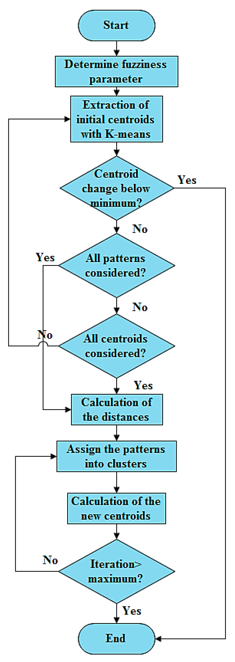
3.5.2. Description of the Algorithm

It should be noted that since data are at the core of the clustering procedure, each sample is modeled differently. Crisp clustering is disadvantageous in cases when there is no clear data structure, in cases of presence of borderline patterns, and finally when the outcome partitions are not easily separable. Soft clustering is a generalization of crisp clustering and involves partial membership over the clusters; this concept is appropriate for handling the degree of fuzziness of the original data. The most widely used soft clustering algorithm is the FCM. The aim is to minimize the following objective function [67,68]:
J ( U , c 1 , , c k ) = k = 1 K J k = k = 1 K [ n = 1 N u n k q d e u c l n k 2 ]
where q [ 1 , ) is the fuzziness parameter and U is the partition matrix. This matrix contains the membership degrees of the patterns to the k clusters. The minimization of Equation (34) is accomplished by modulating the dissimilarity metric as:
J ¯ ( U , c 1 , , c k ; λ 1 , , λ N ) = J ( U , c 1 , , c k ) + n = 1 N λ n ( k = 1 K u n k 1 ) = k = 1 K n = 1 N u n k q d e u c l n k 2 + n = 1 N λ n ( k = 1 K u n k 1 )
where λn, n = 1, …, N are the Lagrange coefficients of the N constrains. The solution of the above equation results in:
c k = n = 1 N u n k q y n m n = 1 N u n k q
u n k = 1 k = 1 K ( d e u c l j k d e u c l n k ) 2 q 1
Equation (37) gives the centroids of the k clusters. In FCM, the clusters’ centroids are obtained by Equation (37). The difference with Equation (27) is the presence of fuzziness parameter q and the element u of the partition matrix. Equation (38) implies that the patterns are assigned to all clusters with a membership degree u. The sum of the k membership degrees u is 1. The value of fuzziness membership influences the results of clustering. Equation (38) gives the membership degree of pattern y n m in cluster Ck. The operation of FCM includes the following phases:
Phase 1.
Randomly select values in the [0, 1] range for the elements of U so that the following constrains are satisfied:
k = 1 K u n k = 1 , 1 n N u n k { 0 , 1 } , 1 n N , 1 k K
where the binary variable unk indicates if the pattern y n m belongs to cluster Ck (unk = 1) or not (unk = 0).
Phase 2.
Calculate the centroids ck, k = 1, , K, with Equation (36).
Phase 3.
Calculate the cost function with Equation (35). Terminate the algorithm if the value of J is smaller than a pre-defined threshold. Else, go to Phase 4.
Phase 4.
Calculate a new matrix U with Equation (36) and go to Phase 2.
FCM is an iteration-based cost function minimization algorithm. While the convergence of the algorithm is not always guaranteed, a series of executions should take place with different initialization conditions [56]. The convergence is accomplished when the pre-defined number of maximum iterations is met or when the improvement of the objective function J between two successive iterations is smaller than a threshold value. In the FCM, unk denotes the degree of membership of the pattern y n m in cluster Ck and consists of the elements of matrix U. This matrix is randomly initialized resulting to the strong dependence of the FCM on the initialization phase. To cluster a specific data sample, FCM should be executed many times, in order to reach a satisfactory result. To overcome this drawback, this study proposes a hybrid and improved version of the FCM. The new algorithm aims at providing a solution to the random initialization problem of the conventional FCM by employing within its operation another clustering algorithm, namely the K-means. Figure 3 presents the flowchart of the improved FCM. The operational phases of the algorithm are described in the following:
Phase 1.
Conduct an initial clustering of Y m for a pre-defined number of clusters (i.e., k) using the K-means algorithm [75]. The initial ck centroids are obtained. Potentially, in this phase every clustering algorithm can be used to produce the initial centroids. K-means is used since it is a fast and efficient algorithm that has been applied to many clustering problems [76,77].
Phase 2.
For each pattern of the set Y m , calculate the Euclidean distances between the patterns and centroids ck.
Phase 3.
Divide each distance dkn with the sum of all distances sum(dkn). Build the matrix U by setting its elements as:
u n k = d e u c l n k s u m ( d e u c l n k )
All elements ukn are within the [0, 1] range.
Phase 4.
Same as Phase 3 of the FCM.
Phase 5.
Same as Phase 4 of the FCM.

4. Simulation Results

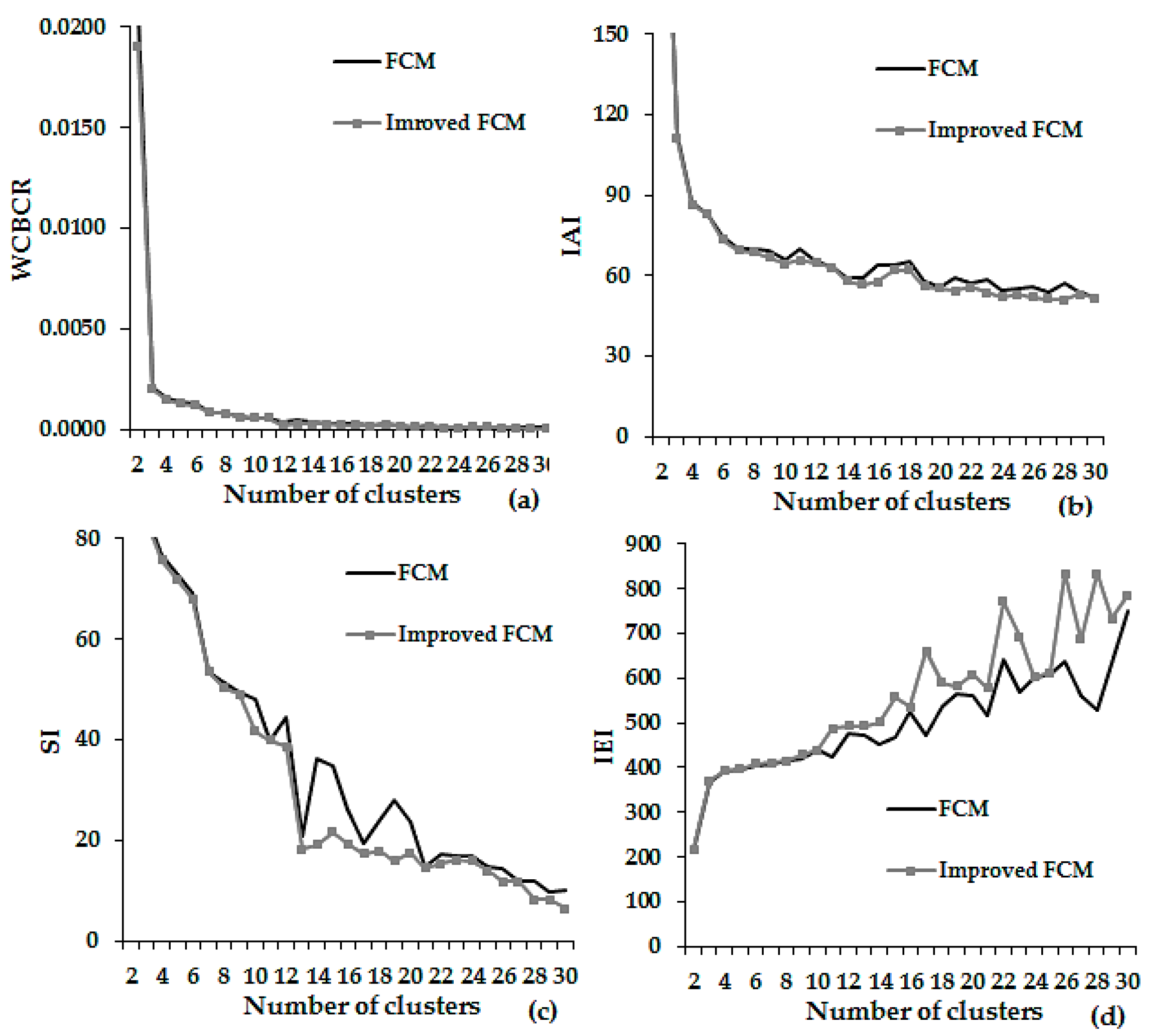
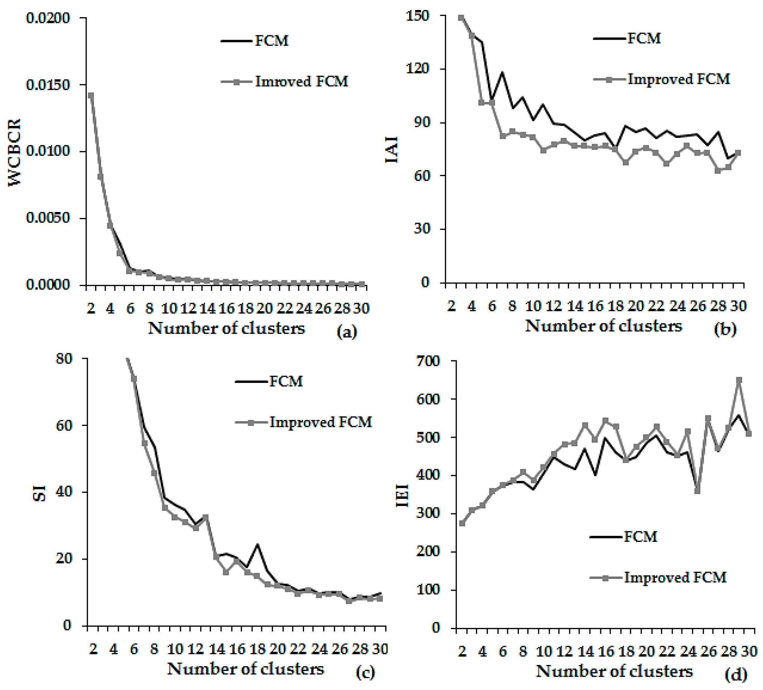
4.1. Load Profiling of HV Consumers

Two (M = 2) existing consumers of the Greek electric sector are considered, i.e., a cement and a steel manufacturing industry. For each consumer, the available data set refer to a period of nine consecutive years and 15 min recordings of the active load are available. A large number of load data strengthens the load profiling conclusions. The consumption of HV industries in Greece is 14% of the total electricity consumption of the interconnected Greek network. This means that the HV industrial sector is a potential candidate for the efficient implementation of load management measures. Such measures may include managing the load patterns in order to reduce or shift the demand from periods of high to low consumption in a beneficial way for both the industry and the distribution SO. Thus, an effective load profiling process can aid in the design and evaluation of sophisticated load management measures. Also, load profiling aids at tracking seasonal patterns, outliers and provides a generic overview of the demand patterns of the consumer. In this section the improved FCM algorithm is compared with the conventional FCM using the load data of the two consumers. No prior external experts information about the number of daily load curve clusters or the data inter-relationships and structures are available, a fact that makes the current load profiling task a purely unsupervised machine one. Also, no pre-processing technique took place such as outlier removal, smoothing, de-trending and others. The soft clustering algorithms are data driven. The number of clusters is determined by a mathematical process applied to the validity indicators shapes. Since, no expertise knowledge about the number of clusters is available, the algorithms should be executed for variable number of clusters. For each cluster number the values of the indicators are checked. The available data for each consumer set covers the period 2003–2011 and refers to hourly load data, i.e., the dimension of patterns is D = 24. Each daily load curve is expressed with a vector with D = 24. Clustering is applied separately in the data set of each year. While the quality of the data was rather acceptable; no outlier removal or missing data filling were employed. Using the maximum and minimum values per year, the normalization technique of Equation (26) is applied separately to the load data per year. The two algorithms are applied to the yearly sets Y m .
Figure 4 and Figure 5 display the comparison of the algorithms using the 2011 data set for consumer 1 (i.e., steel manufacturing industry) and for consumer 2 (i.e., cement manufacturing industry), respectively. The algorithms are executed for two to 30 clusters. A low number of clusters is not desirable, since it results in high clustering errors and therefore the segmentation of the original data set is not proper. On the other hand, a high number of clusters is not recommended since it refers to increased complexity and impose limitations on the load profiling applications, for example DSM, load forecasting and others. To keep the comparison fair, the algorithms’ parameters are kept identical (i.e., fuzziness parameter, objective function improvement threshold and maximum number of iterations). The WCBCR, SI and IAI indicators generally have lower values as the number of clusters is increasing, contrary to the values of IEI. It should be noted that a comparative analysis of clustering with many validity indicators is a common approach in the literature [56]. According to the Figures, Improved Fuzzy C-Means (IFCM) lead to lower clustering errors at all cases. This fact is pointed out by the lower values of the WCBCR, IAI and SI indicators and higher values of the IEI indicator.
The selection of the clustering validity indicator is critical to the conclusions drawn by a load profiling application. The indicators evaluate the algorithms’ performance by measuring the clustering error. The latter refers to the level of similarity of patterns within the same cluster and level dissimilarity between patterns of different clusters. The term compactness or cohesion refers to similarities of patterns of the same clusters and between the patterns and the centroids of the clusters that belong to. The term separation refers to the dissimilarity of the centroids. In the ideal case, an algorithm should result in compact and well-separated clusters. For the purpose of delivering an in-depth comparison between the algorithms, a set of indicators is required. Indicators may measure the compactness, the separation or both of them. The indicators are built upon Euclidean distance, which is a fundamental metric to measure the similarity between two vector patterns. The Euclidean distances between the patterns and the centroids or the centroids themselves of the generated clusters, are expressed by the WCBCR. WCBCR appears as a robust indicator since it assesses both compactness and separation. The distances between the patterns and the centroids tend to decrease while the number of clusters is increasing. This is due to the formation of more centroids that are closer in the feature space with specific centroids. The IAI indicator refers to the sum of the distances between the patterns and the centroids. IAI only measures the compactness of the clusters. As in the case of WCBCR, it displays a decreasing tendency but with a more unstable shape. The SI displays many fluctuations especially in the case of the FCM algorithm. Finally, IEI is a measure of distinctiveness between the centroids and the arithmetic mean of the patterns data set. This distinctiveness is a form of assessing the separation. While the number of centroids is increasing, the number of summations (i.e., between the centroid and mean) increase in number and hence, IEI receives higher values. From Figure 4 and Figure 5 it is shown that the proposed algorithm leads to better clusterings than the original version of the FCM. This is more evident using the IAI, SI and IEI indicators.
The difference between the performances of the two algorithms becomes clearer after the 5th or 6th cluster. Recall that the available data cover the period between 2003 and 2011. The algorithms are executed separately for each year. In order to evaluate the algorithms for the whole period, the mean values of the adequacy measures are used. To clarify this concept, for each year an adequacy measure curve is calculated. Then the mean curve referring to the period 2003–2011 is calculated and utilized for the algorithms comparison. The concept of using the mean values of the indicators that corresponds to subsequent years is useful when dealing with large data sets. It should be noticed that the majority of the load profiling literature presents and evaluates algorithms using sets that cover periods of a year or less [48,51,52]. It is recommended that the usage of large sets supports the reliability of the assessment of a proposed algorithm or methodology. Figure 6 and Figure 7 present the comparison of the algorithms regarding the mean values of the validity indicators.
It is observable that the fluctuations in the shapes of IAI, SI and IEI have been limited. Again in this set of experiments, the improved FCM outperforms the conventional form of the algorithm. Figure 8 is a graphical representation of the shape of a general adequacy measure that shows a monotonic decreasing behavior with the number of clusters. For illustration reasons, the maximum number of clusters is k = 40. In the ideal case, WCBCR, SI and IAI measure are continually decreasing while clustering is performed with higher number of clusters.
After a specific number of clusters, there is a slight decrease of the adequacy measure that corresponds to the “knee” of the curve. In order to derive the optimal number of clusters, i.e., the one that corresponds to the value of measure at the curve’s “knee”, a mathematical process known as the “knee” point detection method is applied, which is briefly described in the following:
Two lines from the points (x2, y2) to (x3, y3) and form the points (x39, y39) to (x40, y40) are drawn. The point of intersection (x, y) of the two tangent lines will give approximately the “knee” of the curve. The value of y (vertical axis) at that point would give the number of clusters of the x-axis. If the value of y does not coincide with the absolute number of x, an intermediate value of x should be considered with equivalent value on the y-axis less near to the derived value of y. The slope intercept of the line is:
y = a + b x
where a is the y intercept and b = Δ y Δ x is the slope of the line. From LINE1 it is:
y 1 = a 1 + b 1 x 1   and   b 1 = Δ y 1 Δ x 1
From LINE2 it is:
y 2 = a 2 + b 2 x 2   and   b 2 = Δ y 2 Δ x 2
The equation of the slopes, the value of x is derived:
a 1 + ( Δ y 1 Δ x 1 ) x = a 2 + ( Δ y 2 Δ x 2 ) x
and since Δ x 1 = Δ x 2 , it is:
x = a 1 a 2 Δ y 1 Δ y 2
The values of points (x2, y2), (x3, y3), (x39, y39) and (x40, y40) are extracted from clustering and using Equation (45) the value of x is obtained.
The output of clustering refers to the centroids expressed in the [0, 1] range of values. The inverse transformation of Equation (27) gives the centroids in physical units, i.e., the load profiles. Apart from assessing the algorithms’ performance, a robust clustering validity indicator should provide information about the optimal number of clusters. Among the validity indicators, WCBCR is more suitable to apply the “knee” point detection method. This is because WCBCR presents a less volatile shape compared to the other indicators. The application of the method to the WCBCR curve as it is extracted by the improved FCM (Figure 4) leads to k = 6 clusters for consumer 1. Also, following the same approach, k = 6 clusters are obtained for consumer 2 (Figure 5) as well. The load profiles of 2011 are illustrated in Figure 9.
Load profiling actually provides a reduction of the magnitude of the original load data set; the initial set of 365 daily load curves is represented now by a reduced set of typical load curves or load profiles. In the present cases, the daily load curves of 2011 are optimally grouped in six clusters and represented by six profiles. According to Figure 9a, a further classification of the profiles into two types can be done. Profiles c#1, c#3 and c#6 refer to a relatively stable demand. No large fluctuations and no sudden peaks are observed. All the other profiles refer to high demand during the first morning and night hours. This is due to the fact of the lower night-time tariffs charges offered by the Retailer to eligible industrial consumers. The industry’s owner takes advantage of the low electricity tariffs offer and shifts the larger portion of the industrial activity during that specific period. The lowest consumption is met during 10:00–14:00 h. Usually, this period coincides with the morning peak of the Greek power system. Afterwards, the consumption is continually increasing. This tariff structure is a basic technique to avoid load congestion in morning peak hours. The load of consumer 2 is higher. In this case, two profiles display a stable form, namely c#1 and c#3. The rest profiles correspond to low consumption during the regular working hours. The selection of a single profile to represent the consumer is a choice that is made by the analyst. A potential selection will refer to the most populated cluster profile that corresponds to the majority of the days of the original data set. Other selections would refer to the profile of the maximum daily energy consumed (i.e., the profile that refers to the larger area covered by the curve), the profile that corresponds mainly on working days, the profile with the peak load and others. It should be noted that the extracted load profiles refer to the year of 2011. In case the database of the consumer is updated with new data, these new daily load curves can be distributed in the existing clusters or a new clustering can take place that will include the new daily load curves within the existing load data set.

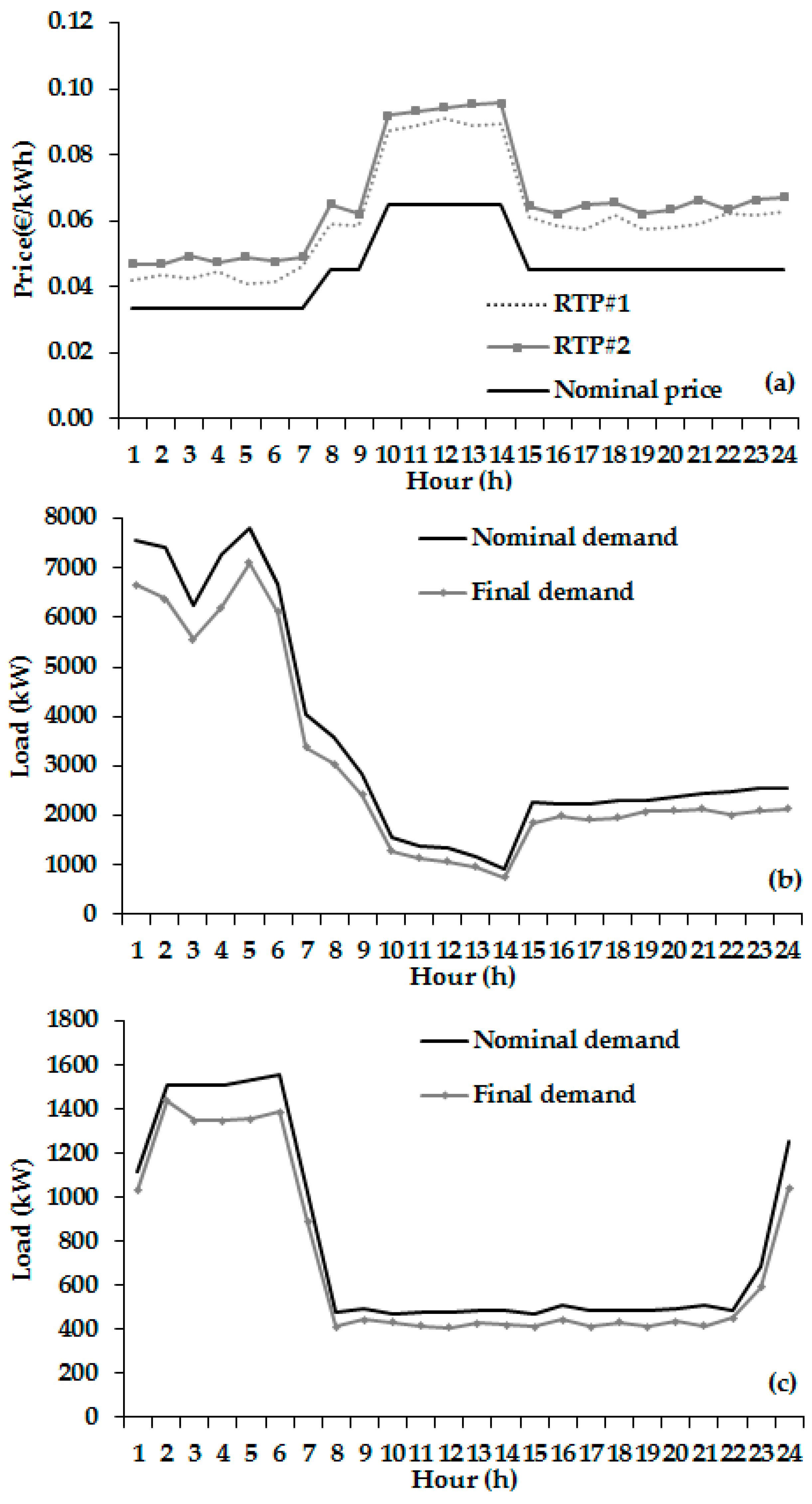
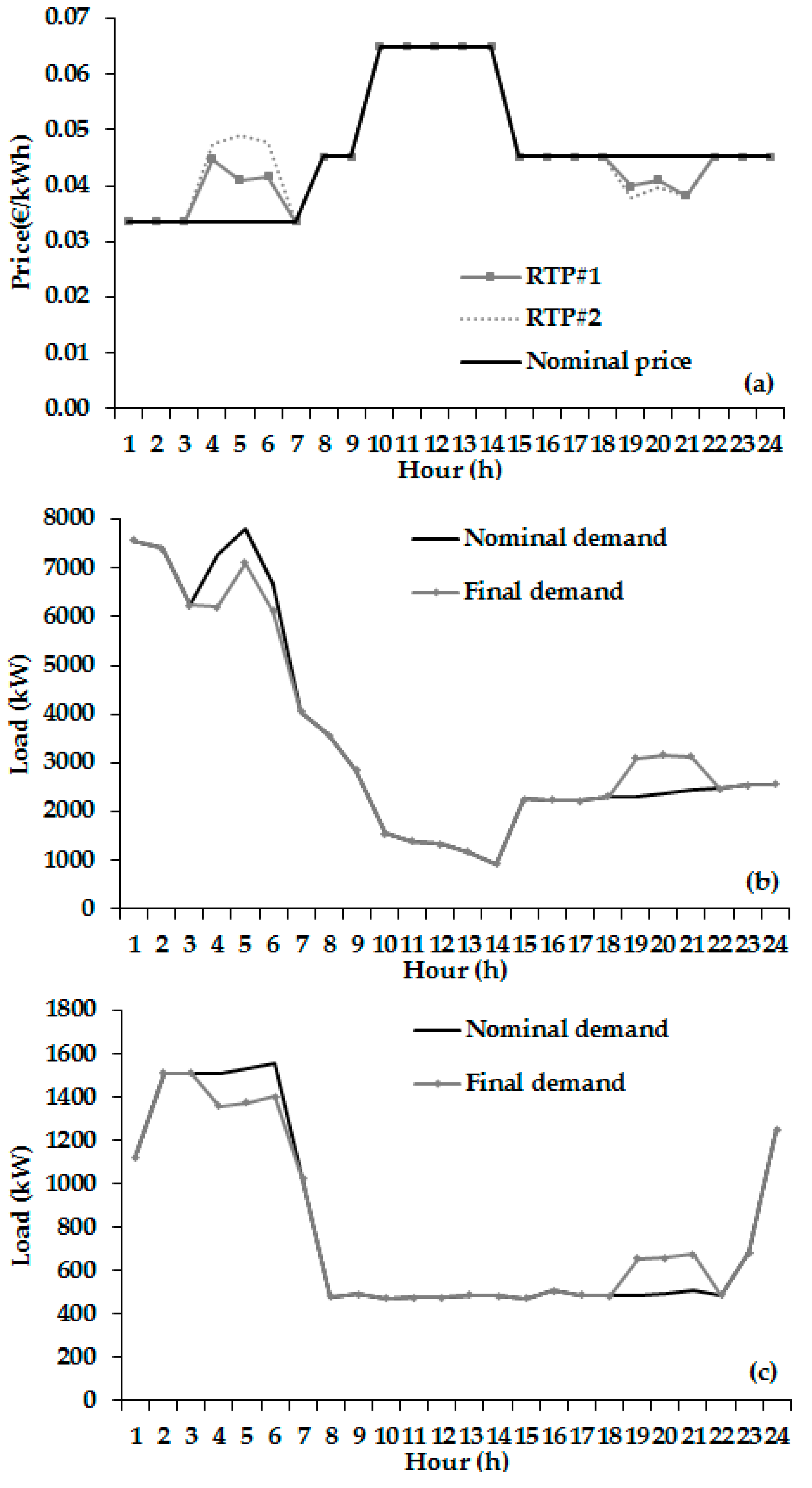
4.2. DSM Objective: SC

The proposed model is applied to a random test day, namely on 8 August 2011, which was the 2nd Monday of August. In the present paper, a novel method is proposed to derive dynamic price elasticities curves, i.e., price elasticities that vary per hour. Figure 10, Figure 11 and Figure 12 show the price elasticity curves of the test day of 2011 considering the linear, exponential and logarithmic models for both consumers, respectively. The procedure to obtain the dynamic price elasticity curves is the following: Clustering is applied to derive the price elasticity of the consumers for the test day under study, based on the similarities of the test day and others days per year. Using the improved FCM for k = 6, all the clusters that contain the 2nd Monday of August of years 2003–2010 are selected. Next, the day type distribution of the selected clusters is checked. Let L t e s t y ,   y = 2003 ,   , 2010 be the cluster labels of test days (i.e., 2nd Mondays of August) in the years 2003, …, 2010, respectively and L t e s t 2011 be the cluster label of the test day of 2011. Also, let S d a y y ,   y = 2003 , , 2010 , d a y = 1 ,   ,   364   o r   365 be the sets that contain the days that belong to the same cluster with test day (i.e., have the same cluster label L t e s t y ) of years 2003, …, 2010, respectively. The days within the sets S d a y y that are same from year to year by employing the intersection are sought, I d a y , of sets S d a y y , I d a y = { S d a y y 2003 S d a y y 2010 } . The days preceding the test day of 2011 are not taken into account in 2011 because they are not known. For instance, I d a y contains days of December of each year are not regarded in 2011. Let I d a y I d a y be the set that does not contain the days that precede the test days of each year. The corresponding days with I d a y of 2011 are gathered in a new set, namely J d a y . Then, using a curve fitting process on the daily load curves of J d a y and p0(h), the parameters alin, blin, aexp, bexp, alog and blog are calculated. The curve fitting models that are applied to estimate the above parameters are the demand functions dlinp(h) = alin + blinp(h), dexpp(h) = aexpebexpp(h) and dlogp(h) = alog + blogln(p(h)), respectively.
The next step is to calculate the hourly price elasticities using Equations (23)–(25) of each day of set J d a y . By averaging the daily price elasticities per hour that are extracted via the fitting process, the hourly price elasticities, i.e., the daily price elasticity curve of the test day of 2011 is derived. According to Figure 10, Figure 11 and Figure 12, consumer 2 is less flexible. The linear model leads to more volatile curves. The logarithmic model leads to more stable elasticity curves with lower values. Values close to zero refer to inelastic behavior. The exponential model leads to price elasticity curves with values that are generally between those of the linear and logarithmic models. It can be concluded that the selection of the DR model affects the derived elasticity curve values.
The purpose of SC is to reduce the overall net-consumption during a period. Usually, this is accomplished by motivating consumers to use energy efficient equipment. In the proposed model, the SC objective is materialized by a RTP program. Although price-based DR programs such as RTP are voluntarily, in the present study it is assumed that consumers respond to all price signals. In the SC objective, ten minutes prior to the hourly RTP signal, nominal loads d 0 1 ( h ) and d 0 2 ( h ) are known to the Retailer. For the test day under study an hourly reduction of R(h) = 10% is assumed. The upper limit of prices is set to u(h) = 150%, i.e., the offered prices derived by the optimization problem, p1(h) and p2(h), should not exceed by 50% the nominal price p0(h). Price limits can be set by the Retailer or the regulatory authority reflecting market competition and conditions. SO has no influence on the pricing policy of Retailer. Extremely high prices may lead to consumer not complying with the price signals. The parameters R(h) and u(h) can vary per hour. In the present test case, they are considered unchanged within the 24 h period of the test day. Thus, a total 10% reduction objective applies for each hour. Other potential SC objectives may refer to an average 10% reduction per day or to a 10% reduction per consumer. The scope is to derive the RTP profiles that will lead to the reduction target. Prices p1(h) and p2(h) refer only to the electricity cost. Additional expenses during the operation of the Retailer can also be included. The optimization problem is solved hourly and separately for each demand function. Prices p1(h) and p2(h) obtained by the solution are sent to consumers. The responses or final demands d1(p1(h)) and d2(p2(h)) are calculated after the termination of the DR event.
Figure 13 presents the results of the SC objective employing the linear DR model. The nominal daily price profile is depicted in Figure 13a and is common for both consumers. The RTP profiles of the two consumers refer to variant prices that are higher than the nominal ones in order to bring forth the desirable SC objective. RTP#1 corresponds to consumer 1 and includes lower charges than RTP#2 that is applied to consumer 2. The price elasticity profiles play a significant role in the determination of the RTP. As reported by Figure 10, Figure 11 and Figure 12, consumer 1 is more sensitive to prices and thus, lower electricity charges can be applied. In addition, due to its elastic behavior, at least theoretically, consumer 1 should contribute to the largest part of the 10% reduction target. The two consumers do not only differ in terms of load profiles and load magnitudes, but also in terms of price elasticity profiles. The more flexible is the demand the higher deviations from the nominal demand are expected. It can been observed from Figure 13a that both RTP profiles generally follow the pattern of the nominal profile. The latter profile aims at formulating a demand pattern to HV consumers that is poorly correlated with the one of the interconnected system of Greece. The scope is to shift HV loads to system’s low consumption periods. Contrary to the nominal price profile that is a typical TOU rate tariff, RTP profiles vary per hour presenting a more accurate and fair pricing policy to the HV consumers. RTP has the potential to deliver all the different DSM objectives. Also, by linking RTP with system marginal prices of the wholesale market, the actual generation costs can be transferred to the consumers. The nominal and final demands of the two consumers are shown in Figure 13b,c. The reduction levels are in accordance with the RPT profiles variations. Each consumer contributes to the reduction target by a different share that depends on the price elasticity and offered price. It is shown that the SC objective is successfully manifested. The first morning and the late night hours correspond to higher consumption periods. Consumption progressively decreases until 08:00 h and remains low until midnight. Afterwards, the consumption increases again. The higher share for delivering the 10% of total initial load reduction target refers to consumer 1. This share varies per hour. The daily average is 79.97%. Figure 14 and Figure 15 present the results considering the logarithmic and exponential DR models, respectively.
The comparison between the various DR models is held in order to examine whether the selection of different DR model influence the SC objective success at delivering the predefined level of reduction set out by the SO. To keep the comparison feasible, the same load reduction R(h) and price limit u(h) are kept for all DR models. The logarithmic DR model leads to different contributions to the reduction target by the consumers. The highest one is met during the peak hours. This is because of the high deviation of the RTP from the nominal price. Recall that apart from the level of the offered price, price elasticity is a critical parameter for the fulfillment of the DSM objective. Again, consumer 1 accounts for the largest share in the reduction target. In the logarithmic model, the price profiles follow more strictly the pattern of the nominal price. In the exponential DR model, the price elasticities profiles display a correlation in the shape with the nominal price profile. This model leads to prices that lie between the other models. All models lead to the fulfillment of the R(h) = 10% target.
The difference among the models lies in the price profiles and the contributions of the consumers to the target. In addition, the upper price limit u(h) = 150% is never reached. Apart from the price profiles shapes, each model leads to prices that differ in terms of magnitudes.

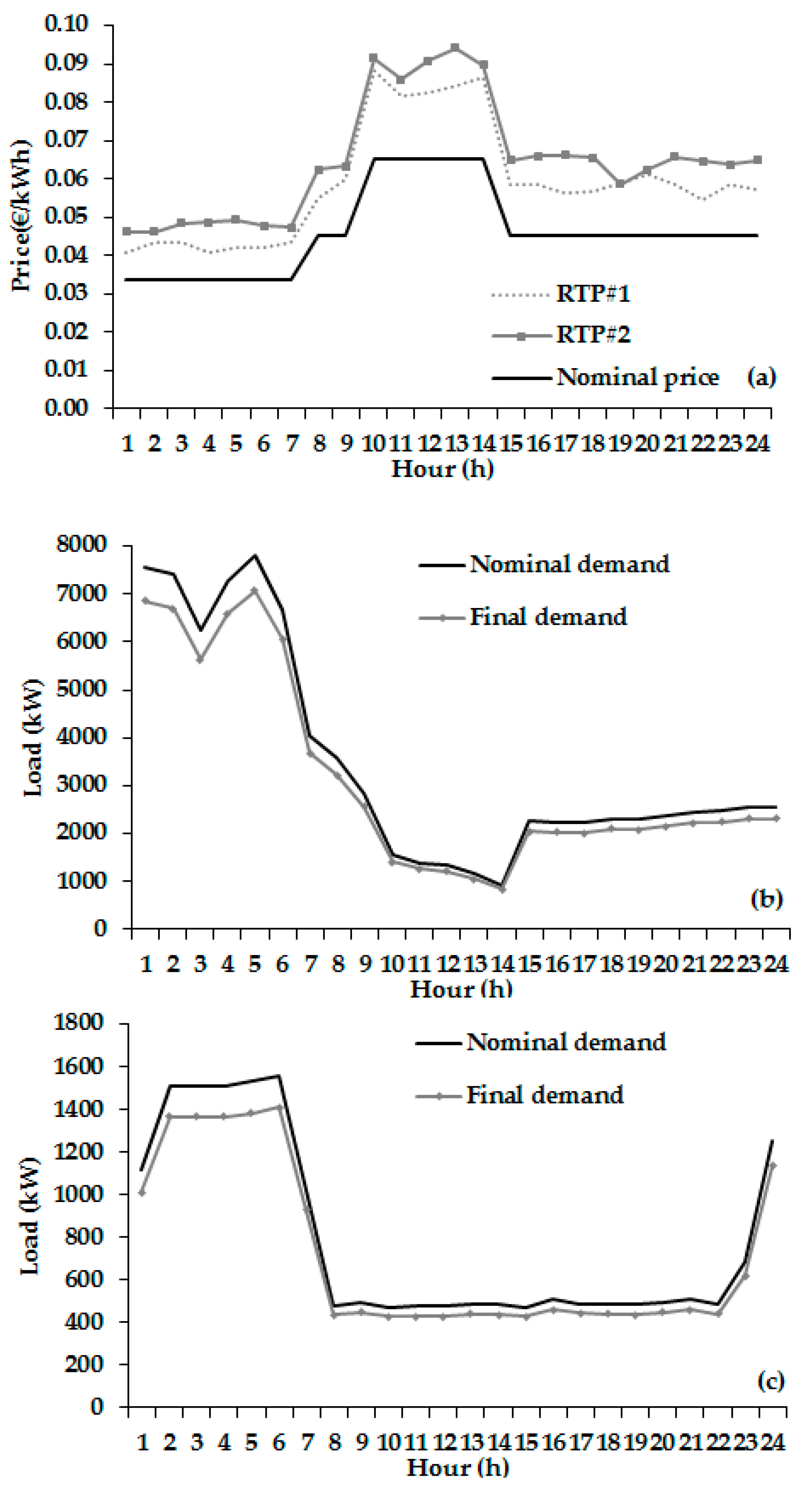
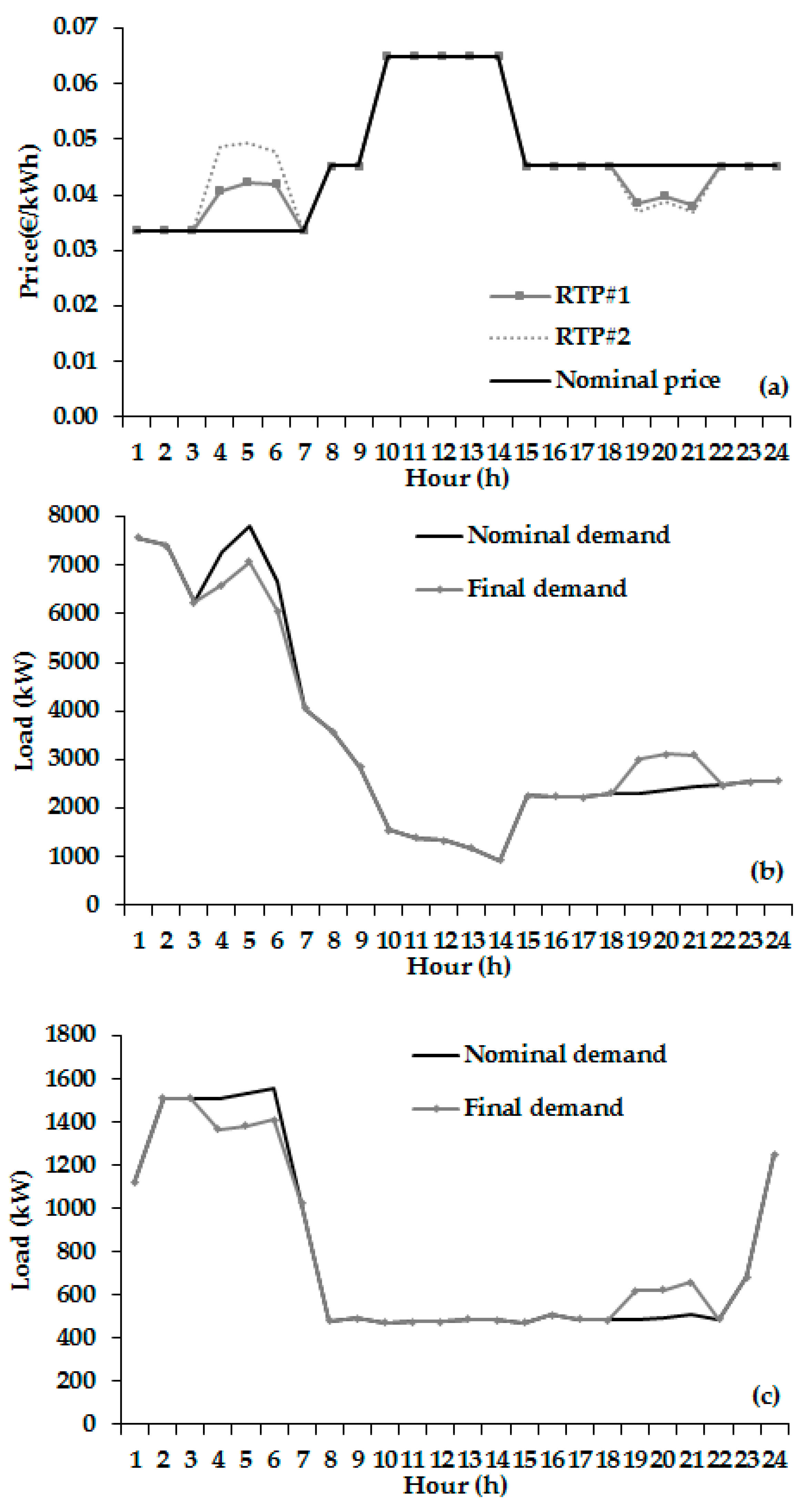
4.3. DSM Objective: LS

LS refers to the phenomenon of shifting loads from on-peak to off-peak periods. While the peak demand is increased, there is no changes in the total consumption. Peak loads that are cut are summed to loads of off-peak hours. In the present test case, the net electricity consumption remains unchanged; the amount of load that is cut from on-peak hours equals the one that is added to the off-peak hours. The LS objective can be combined with a SC option; the peak load that is shifted would not be equal to the load that is summed to the off-peak loads since a peak load reduction phase would precede the load filling event.
The LS objective is a combination of two DR events: A load reduction by 10% in hours 04:00, 05:00 and 06:00 h and a load increment in hours 19:00, 20:00 and 21:00 h. The load that is removed from the morning hours is aggregated to the existing loads of 19:00, 20:00 and 21:00 h. While hours 19:00, 20:00 and 21:00 h refer to off-peak hours, they do not refer to the lowest daily consumption. The two consumers present the lowest consumptions in different periods, the above hours since they refer to low consumption for both consumer are selected. However, it is feasible for the proposed model’s operation to regard different load filling periods per consumers and more than one peak load shaving and load filling periods per consumer. In the LS objective, the duration of the two DR events is the same, each one lasts 3 h.
Figure 16 present the results of the LS considering the linear DR model. The price profiles of the LS objective using the logarithmic demand function are displayed in Figure 17a, while the nominal and final loads of the consumers are shown in Figure 17b,c, respectively. Figure 18 presents the results of the LS objective using the exponential model. In the present test case, an hour per hour shifting is employed, i.e., the load from 04:00 h is aggregated to the load of 19:00 h, the load from 05:00 h is aggregated to the load of 20:00 h and the load from 06:00 h is aggregated to the load of 21:00 h. This per hour load matching concept is held per consumer.
Also, the LS is held consumer-wise, i.e., the load of 04:00 h of consumer 1 is aggregated to the load of 19:00 h of consumer 1, etc. However, different combinations can also be applied. It is not obligatory for instances i, i’ and i’’ to have equal duration as long as the condition I(i’) + I(i’’) ≤ R(i’) + R(i’’) is satisfied. The load reduction amount can be distributed in various periods of the day.
In order to achieve the LS objective, prices at 04:00, 05:00 and 06:00 h should be higher than the nominal ones and prices at 19:00, 20:00 and 21:00 h should be lower, so that the consumers increase their consumption. Price limits are set to u(i) = 150%, u(i’) = 90% and u(i’’) = 90%.
RTP profiles differ from the nominal only during the instances of load reduction and load increment. This is also the case for the final loads. Since consumer 1 is more sensitive to prices, it is offered a lower price. The GA utilized for solving the optimization problem results in slightly different outputs, i.e., prices p1(h) and p2(h), if executed a few times. This is an inherent characteristic of the GA. The initialization of the chromosome populations is done randomly and therefore, different executions of the algorithm lead to different outputs. To keep the comparison with the SC objective practical, prices of the peak shaving event, p1(i) and p2(i), are kept equal to the corresponding hours of the SC objective p1(h) and p2(h). As in the case of SC objective, the upper price limit u(i) = 150% is never met by the solution of the optimization problem.
Also, the upper price limits during the load filling events, u(i’) = 90% and u(i’’) = 90%, are not met. Consumer 2 is offered higher price during the peak shaving event and lower price during the load filling event. As in the case of the SC objective, the exponential model results in prices that lie between those of the other models.

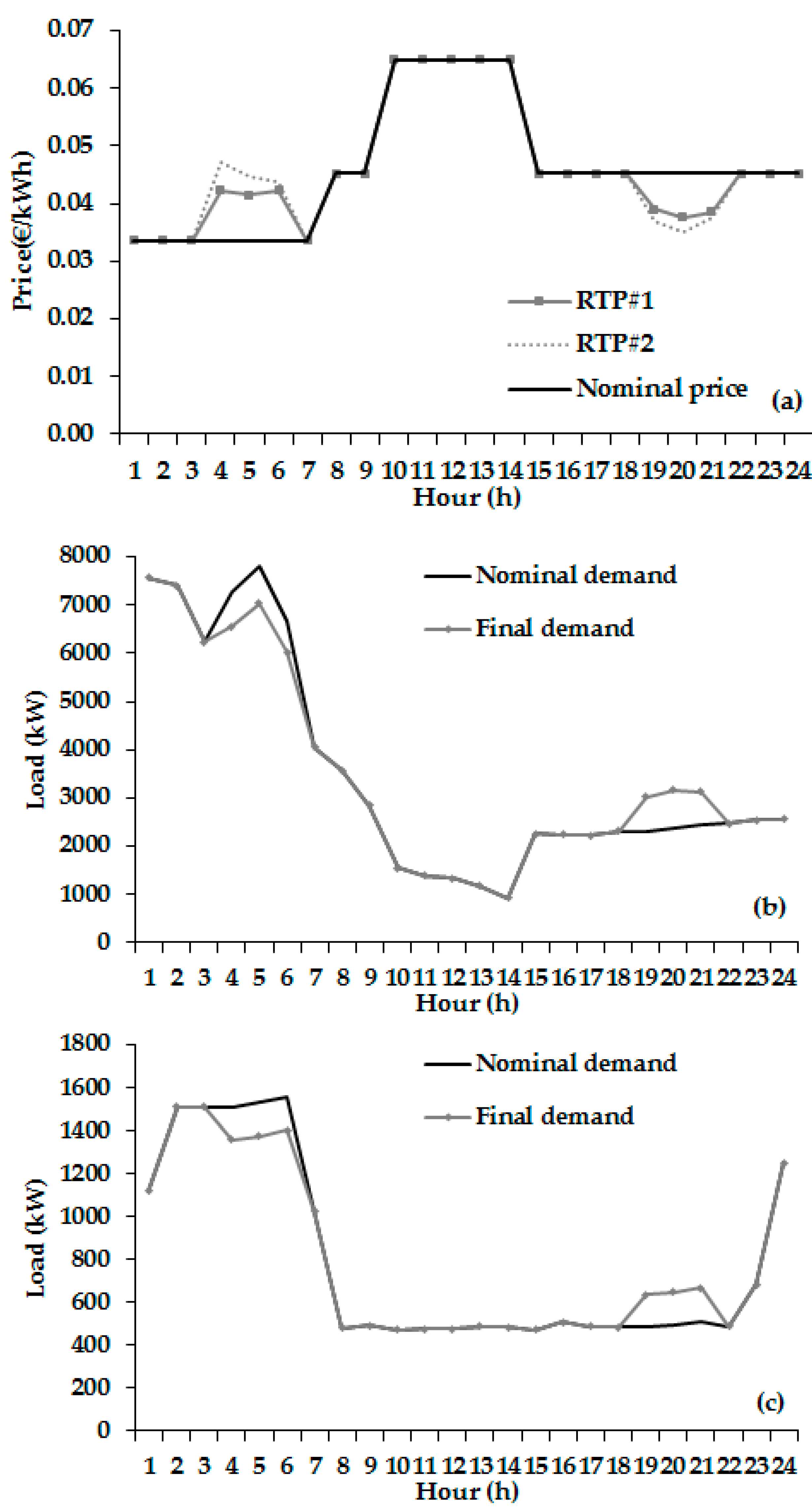
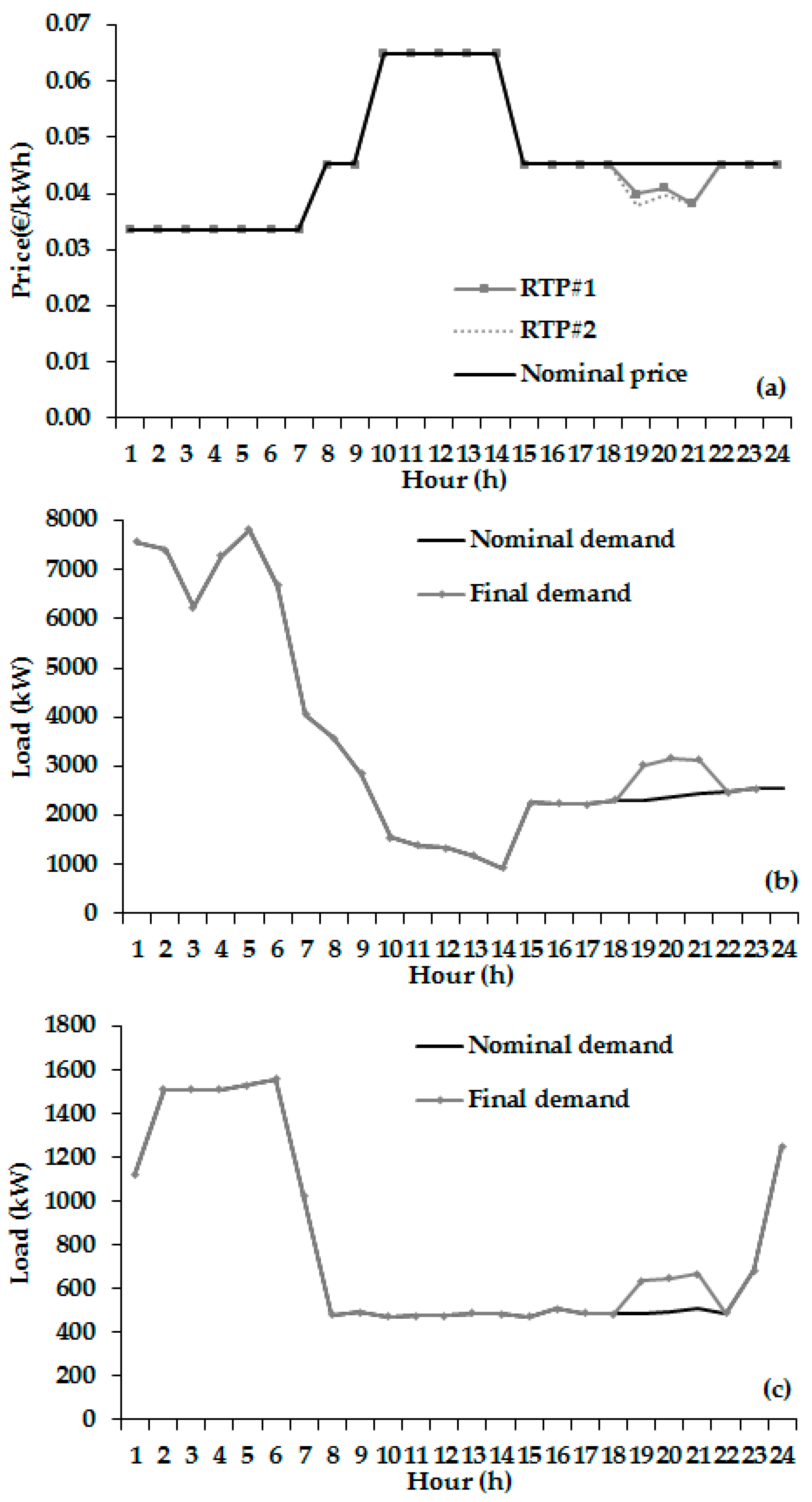
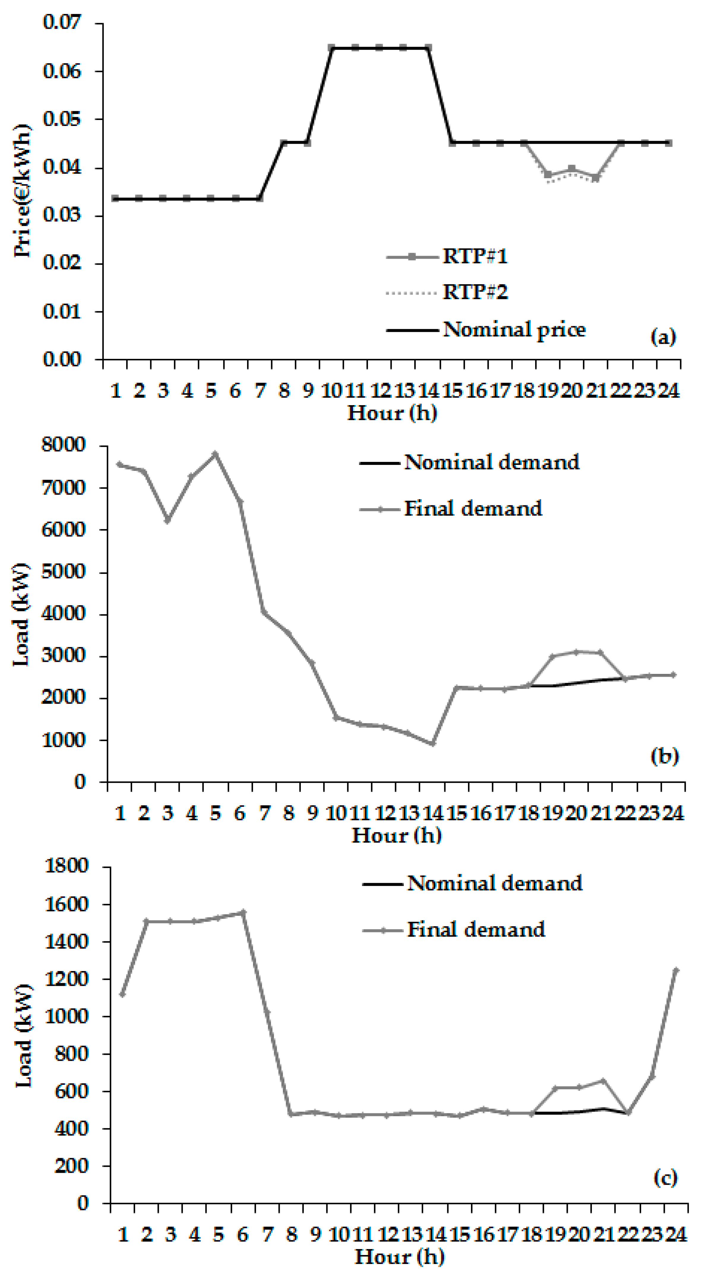
4.4. DSM Objective: VF

Figure 19, Figure 20 and Figure 21 present the results corresponding to the linear, logarithmic and exponential models, respectively. A VF objective can be combined with other DSM objectives or exercised solely. During the VF event, consumers are encouraged to increase consumption during low system’s demand. The goal of the VF objective is to build up off-peak loads in order to smooth out the load and achieve higher load factor ratios. To achieve a VF objective, the Retailer sends lower price signals to consumers. The VF event is employed at 19:00, 20:00 and 21:00 h for both consumers, thus the event includes three consecutive hours. All models achieve the 10% load increment target. In the linear model, the offered prices are reduced by 13.77%, 16.64% and 14.87% with respect to the nominal price at hours 19:00, 20:00 and 21:00 h for consumer 1, respectively and by 18.19%, 22.61% and 16.73% for the same hours for consumer 2, respectively. While in the formulation of the proposed model, prices can be reduced to zero, extremely low prices may lead to poor profits for the Retailer and are not a good practice within the retail energy market competition. Hence, a lower limit should also be placed.

5. Conclusions

Due to the various benefits of DSM in the operation of electric power systems, many utilities and system operators focus on the application of DSM programs for lowering the risks of generation shortage and network congestion. In the present paper, the DSM is regarded as a resource in day-ahead energy market. A novel model has been proposed for achieving predefined DSM targets by using RTP schemes. Apart from the prices that lead to the achievement of the target, the model derives the contribution of the DSM target to the consumers based on their price elasticity.
Another contribution of the paper is the development of a novel soft clustering algorithm that leads to more robust clusters compared with the most commonly used soft clustering algorithm of the machine learning literature, i.e., the FCM. The new algorithm does not increase the complexity of the load profiling problem in terms of input parameter requirement prior to its execution. The new algorithm is a part of the new method for extraction dynamic price elasticities curves. Time variant price elasticities offer a more representative technique to simulate the consumer’s response to RTP programs. Regarding the load profiling analysis, the major findings of the article can be summarized in the following points:
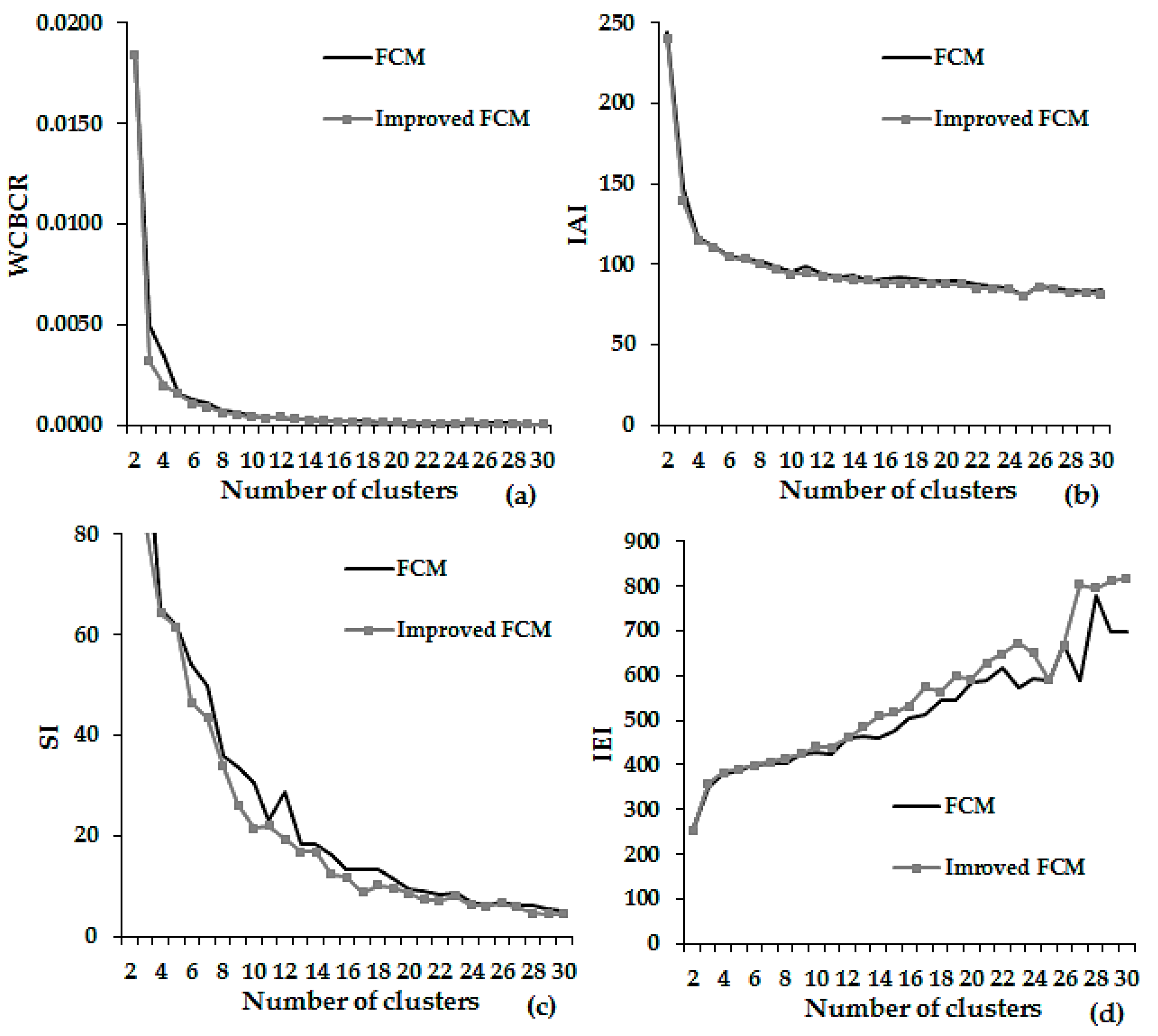
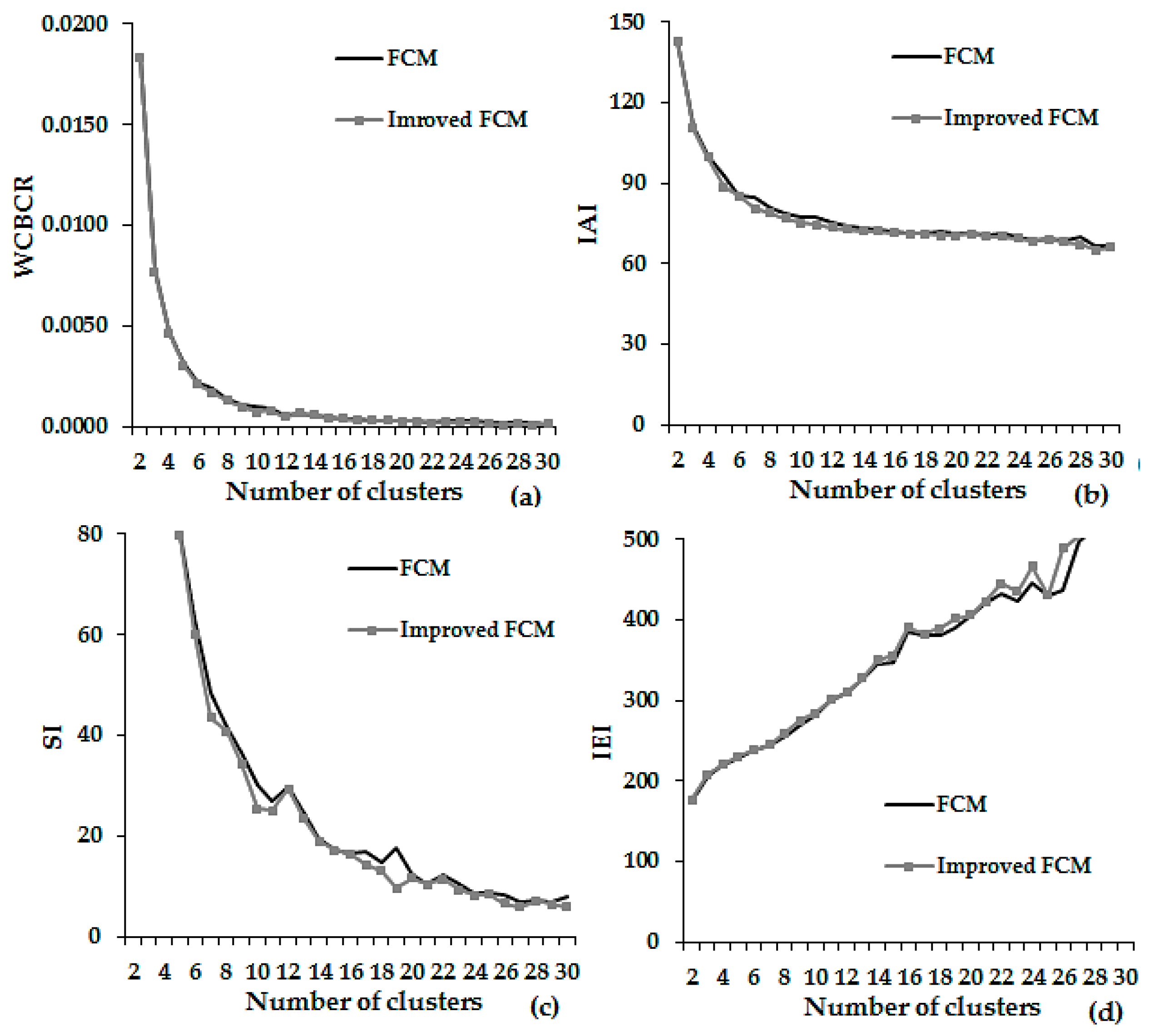
  • In all cases examined, the proposed FCM algorithm leads to lower clustering errors. Therefore, a specific initialization formula of the partition matrix is favorable over the random one as it is the case in the conventional form of the algorithm. The K-means algorithm was used for the initialization due to its proven efficiency in many clustering problems. However, virtually every clustering algorithm can be used.
  • It is necessary to include a variety of assessment criteria to reach safe conclusions regarding the superiority of the algorithm. The criteria can be categorized into two types: (a) mathematical indicators that measure the Euclidean distances; and (b) parameters that are related with complexity. The term complexity may refer to a wide range of definitions. If complexity is related with required execution time, the time elapsed to run the algorithm for variable number of clusters expresses the suitability of an algorithm. The two algorithms compared in the paper, lead to comparable execution times. The conventional form of the algorithm is slightly faster since the proposed FCM includes an initial clustering with the K-means. If it is required to decrease the execution time of the proposed algorithm, it is recommended to use hierarchical agglomerative clustering algorithms instead of the K-means. Also, if the complexity is expressed as input parameters requirements to be defined prior to the execution of the algorithm, the proposed algorithm needs two additional parameters to be set by the user: (a) The objective function improvement threshold of the K-means and (b) the number of iterations of the K-means.
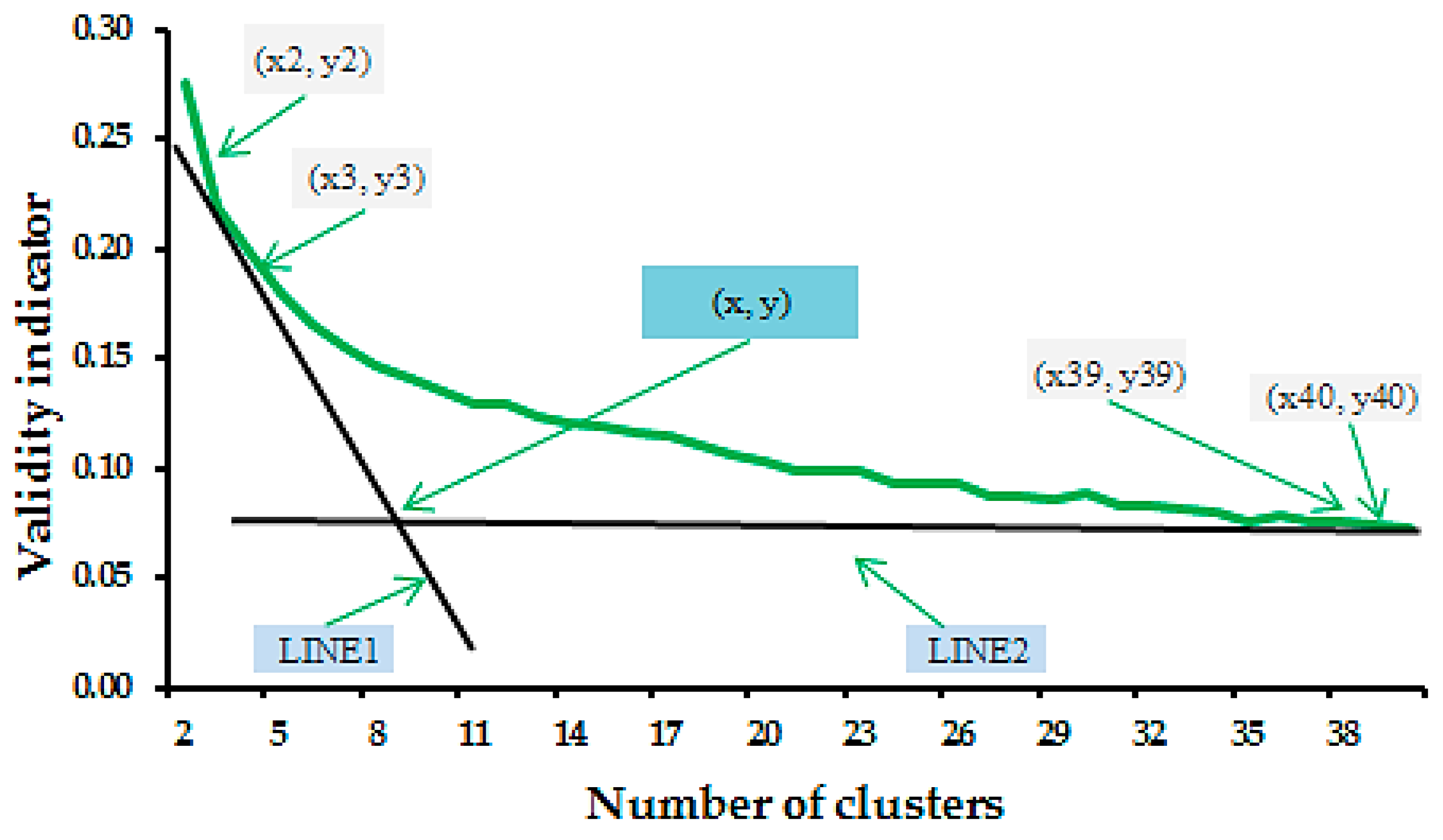
  • A variety of indicators have been used for the algorithm comparison. These indicators can be found in the load profiling-related literature. A reliable indicator should provide information about the optimal number of clusters. Theoretically, the optimal number of clusters is the largest possible. But in practical terms the number of optimal number should satisfy two contradictory conditions: (a) low clustering error and (b) number of clusters with considerable number of patterns. A large number of clusters are generally not recommended as it increases the difficulty of the exploitation of the clustering results. Among the indicators used in the study, the WCBCR measure is suggested. This is due to the following reasons: (a) it exhibits a decreasing tendency that it some cases it becomes monotonic and therefore, it is suitable for the application of the “knee” point detection method and (b) it measures both the compactness and the separation of the generated clusters. The IEI measure is the least suitable due its volatile shape. Both SI and IAI are preferred if the WCBCR is not considered.
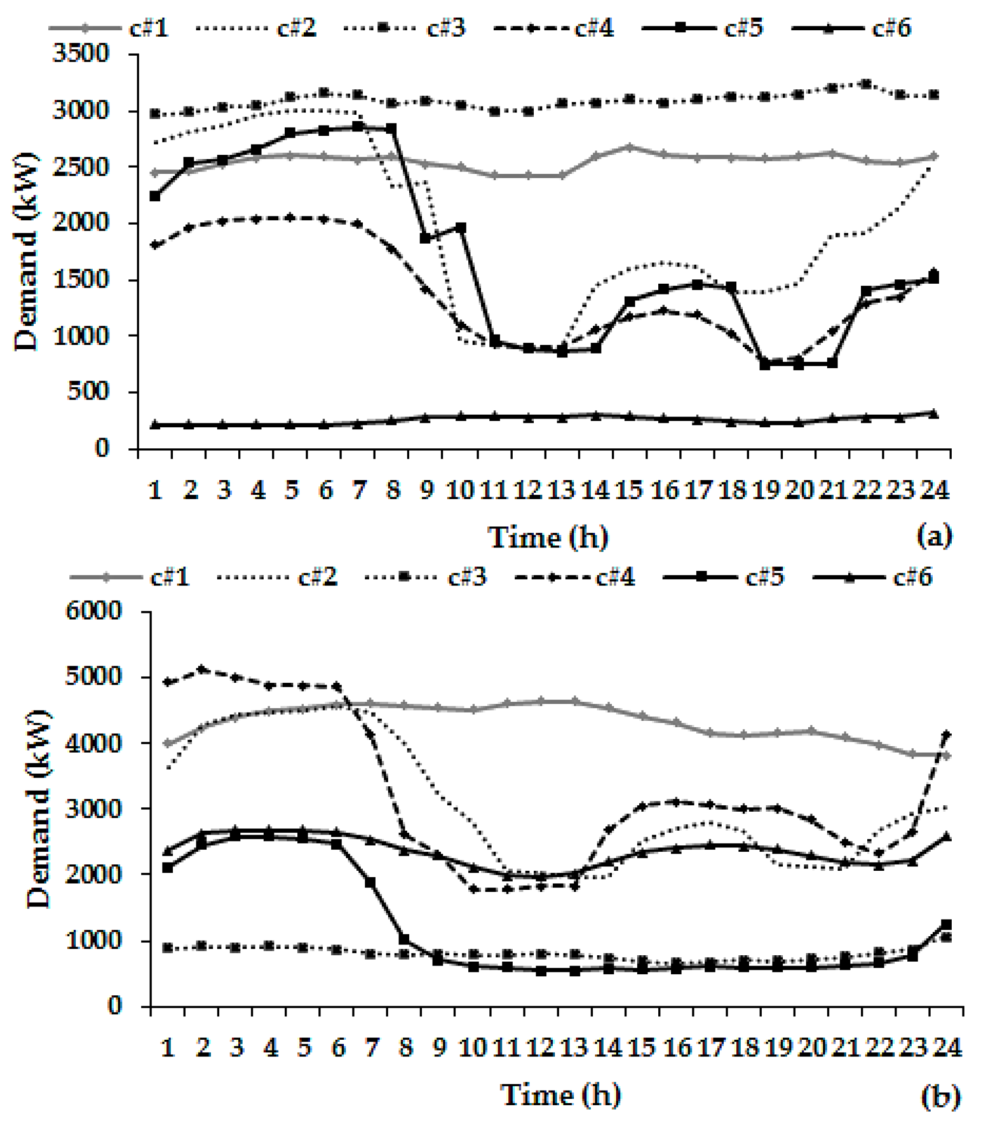
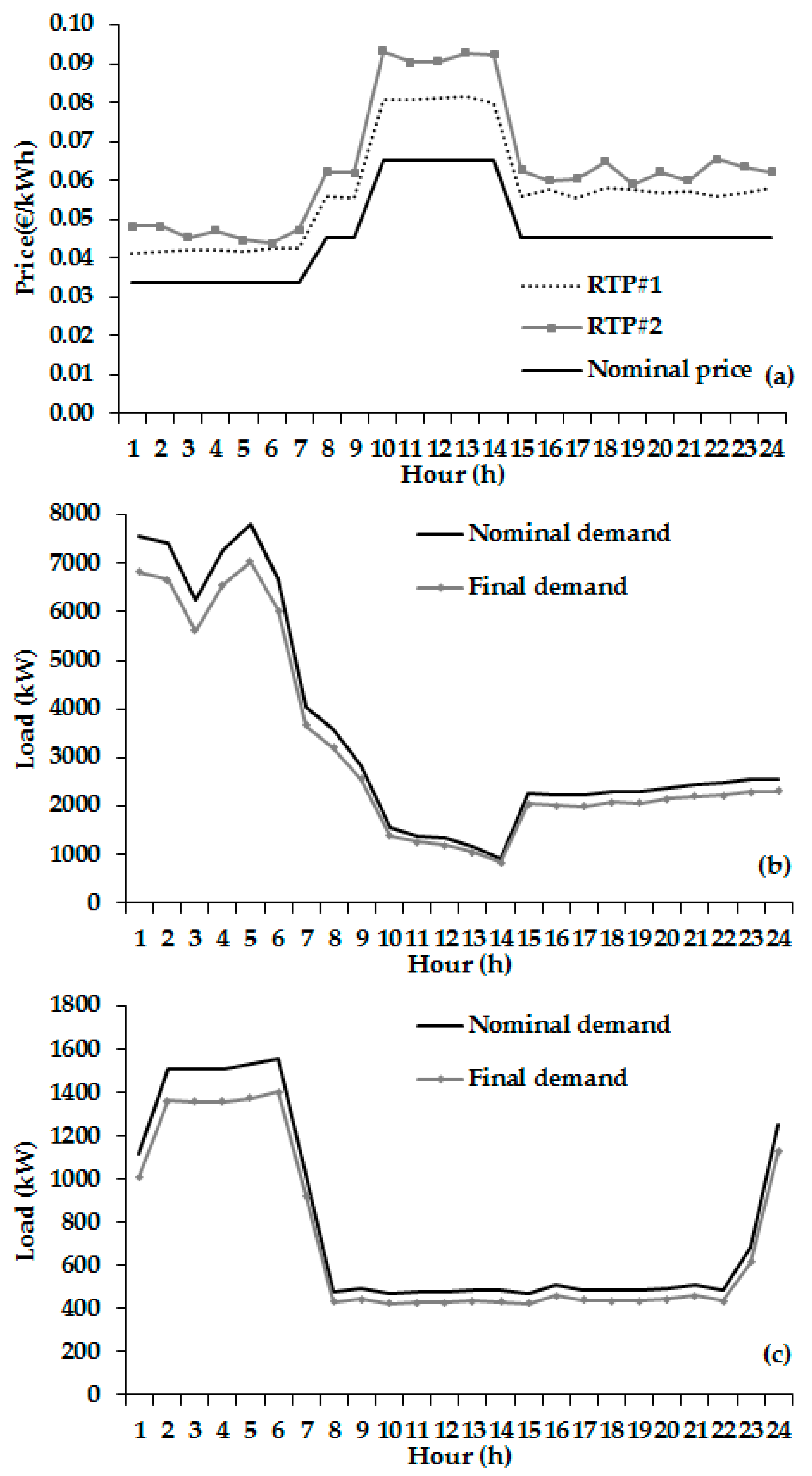
  • The optimal number of clusters for both consumers is below 10. According to the shapes of the load profiles, the demand is high during night hours, again due to the nominal tariff structures. The load profiles do not display sudden peaks.
Regarding the proposed method for deriving the dynamic elasticity curves, the findings of the paper are gathered in the following statements:
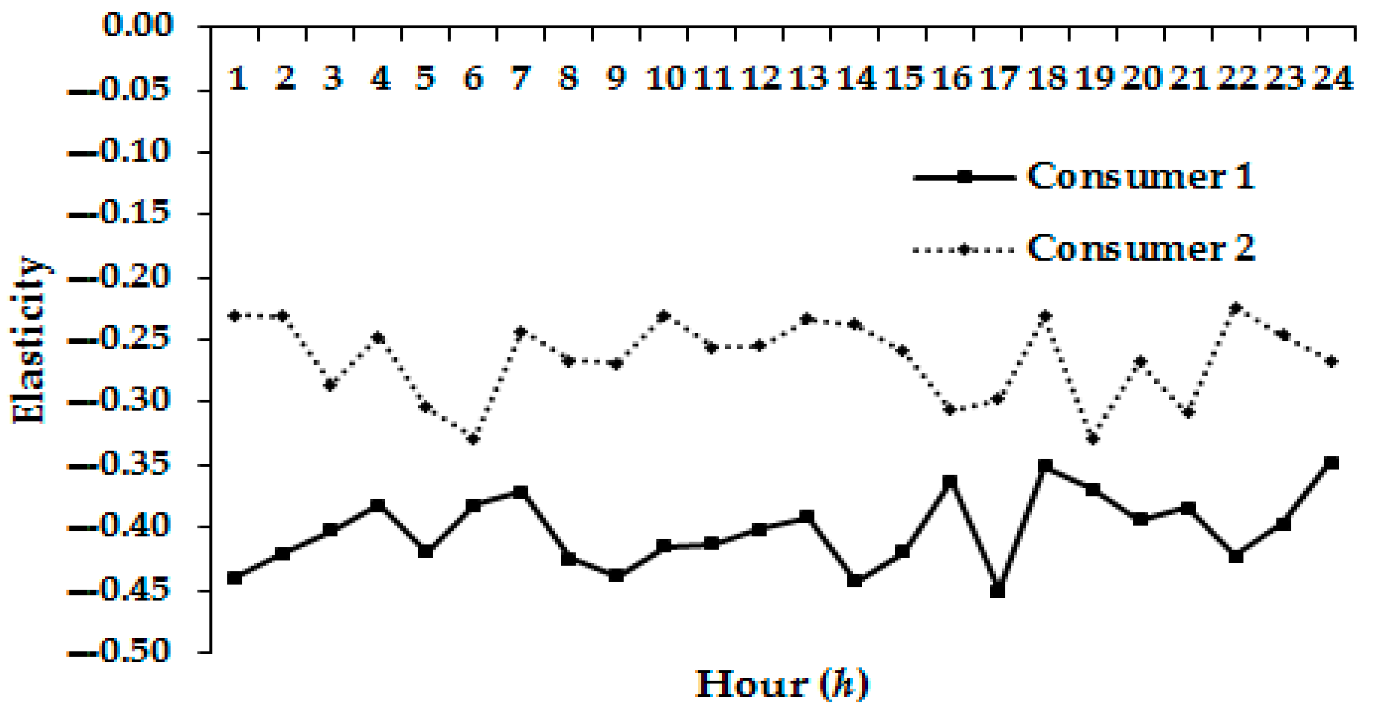
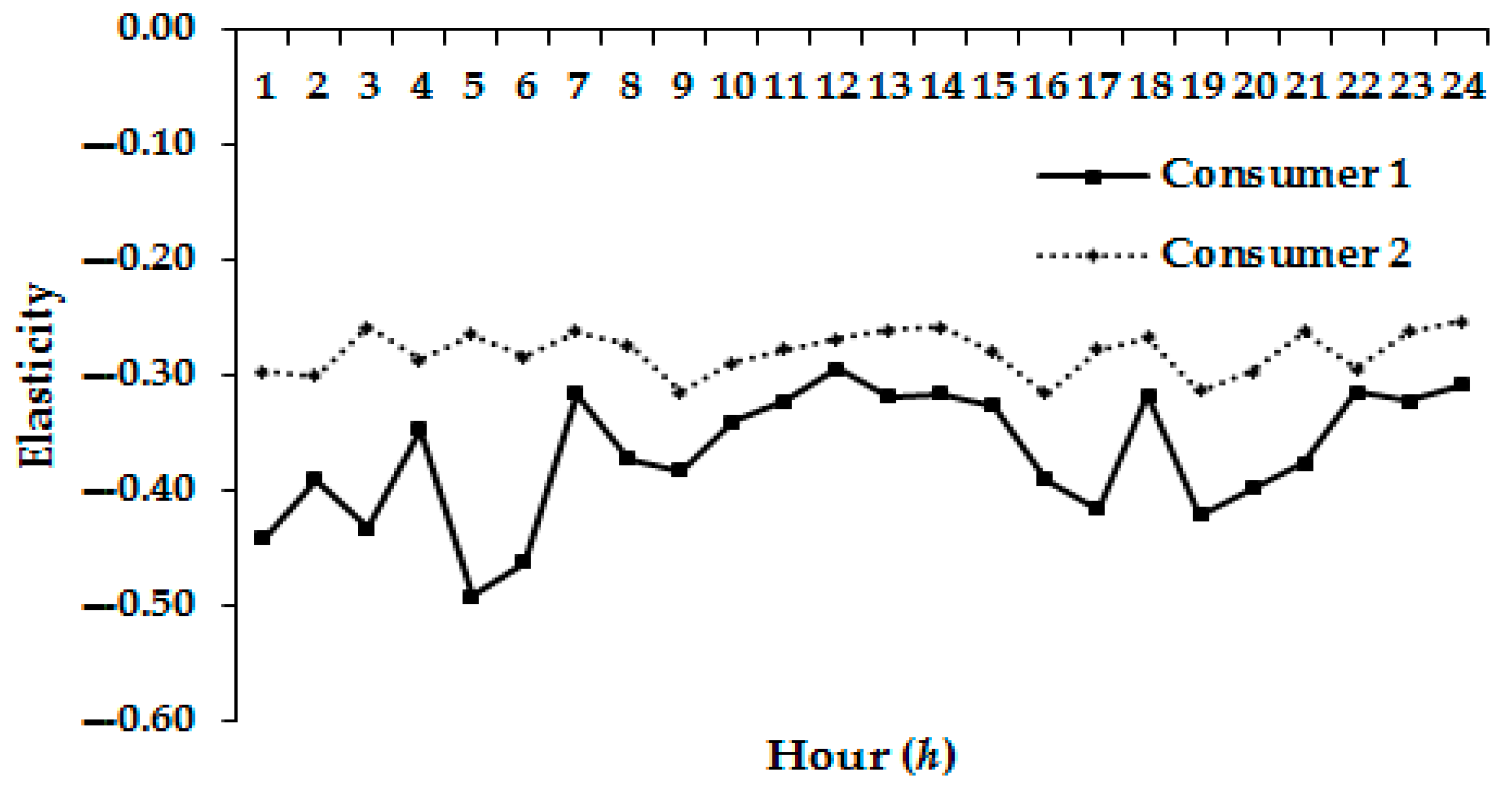
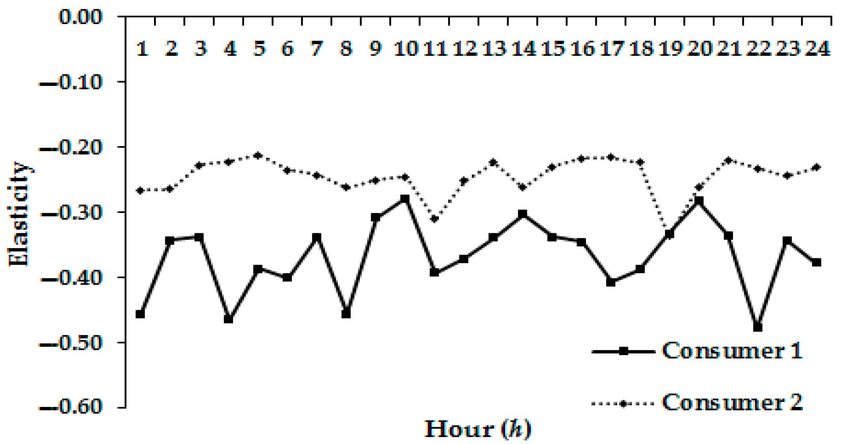
  • In order to derive the price elasticity curves, it is recommended to use data that cover all seasons within the year. The weekly and seasonal variations of the demand changes with respect to prices are included if the calculation covers all seasons.
  • The type of the DR model affects the price elasticity curves. The linear DR model results in lower values of price elasticities. It can be noticed that there are large differences between the hourly values. This is more evident in Consumer#1. Therefore, it is recommended to form consumer specific curves instead of using pre-defined constant values.
  • To provide a robust modelling of the demand behavior, it is recommended to update the price elasticity curves periodically or in special cases of demand changes. For instance if large demand variations are observed or expected due to various reason, prior to the implementation of a DSM objective, a re-calculation of the hourly elasticities is advised.
The concluding remarks after the examination of the experiments held by the proposed model are gathered in the following paragraphs:
  • The formulation of the optimization problem is robust; in all cases examined reaches into feasible solution that satisfy the limitations imposed by the user.
  • All the DSM objectives presented in Figure 2 can be implemented in the model. Three cases have been examined. The prices offered by the Retailer depend on the price limits, the type of the price/demand function and the type of model used to derive the price elasticity curves. The elasticity is the most significant factor that determines the level of success of the DSM objective. A careful selection of price limits makes a Retailer competitive within the retail market competition.
  • The proposed model makes it feasible to achieve a DSM goal with no intervention in the apparatus of the consumers. It is up to the consumer to decide which loads will be cut off or shifted within the daily period. Therefore, the industrial consumer has more control upon its equipment and production processes.
  • The proposed model is highly flexible and can be applied to various types of consumers (e.g., buildings, residential consumer clusters and others). Also, different pricing schemes can be included, such as TOU rates as long as result in the satisfaction of the DSM target.
The present research can be expanded into the following areas:
  • In the case of the load profiling, dimensionality reduction techniques can be examined such as principal component analysis, for the purpose of lowering the clustering execution time. The patterns can be represented with a reduced set of features and this concept, at least theoretically, should reduce the clustering duration. This would be more noticeable in cases with large amounts of data gathered by smart meters.
  • To modify the proposed model in order to simulate the Retailer’s economic benefit. For instance, the demand reduction level in the SC objective can be negotiable among the System Operator and the Retailer. If the SC objective is partially fulfilled a penalty can be applied in the Retailer.
  • Another expansion of the model should take into account cases where self-production units, such as biomass or photovoltaics in the part of the consumer are present.
The model developed in this study is characterized by simplicity. The execution time lasts few seconds in a common computer configuration. Thus, it has the potential to be included in the Retailer’s decision making portfolio.

Acknowledgments

This work was supported by the State Scholarships Foundation of Greece in the context of the IKY FELLOWSHIPS OF EXCELLENCE FOR POSTGRADUATE STUDIES IN GREECE—SIEMENS PROGRAM.

Author Contributions

Ioannis Panapakidis performed the research and wrote the paper. Nikolaos Asimopoulos provided guidance for the research. Athanasios Dagoumas revised the paper. Georgios C. Christoforidis revised the paper and set the objectives.

Conflicts of Interest

The authors declare no conflict of interest.

Nomenclature

SymbolDescription
mConsumer index
MTotal number of consumers
nDay index
P(n,M)Total consumption in day n
DDimension of vector
x n m Daily load curve vector in physical units of consumer m
hHour index
p0(h)Nominal price in hour h
d0(h)Nominal demand in hour h
p1(h)Price in hour h of the 1st consumer
p2(h)Price in hour h of the 2nd consumer
d(p(h))Demand in hour h
p(h)Price in hour h
dlin(p(h)Demand in hour h according to linear demand function
alinCoefficient of the linear demand function
blinCoefficient of the linear demand function
d 0 l i n ( h ) Nominal demand in hour h according to the linear demand function
B 0 l i n ( h ) Nominal consumer benefit in hour h according to the linear demand function
dlin(p(h))Demand in hour h according to the linear demand function
Bc(dlin(p(h)))Consumer benefit in hour h according to the linear demand function
Elin(h)Hourly price elasticity according to the linear demand response model
dexp(p(h))Demand in hour h according to the exponential demand function
aexpCoefficient of the exponential demand function
bexpCoefficient of the exponential demand function
d 0 e x p ( h ) Nominal demand in hour h according to the exponential demand function
B 0 e x p ( h ) Nominal consumer benefit in hour h according to the exponential demand function
dexp(p(h))Demand in hour h according to the exponential demand function
Bc(dexp(p(h)))Consumer benefit in hour h according to the exponential demand function
Eexp(h)Hourly price elasticity according to the exponential demand response model
dlog(p(h))Demand in hour h according to the logarithmic demand function
alogCoefficient of the logarithmic demand function
blogCoefficient of the logarithmic demand function
d 0 l o g ( h ) Nominal demand in hour h according to the logarithmic demand function
B 0 l o g ( h ) Nominal consumer benefit in hour h according to the logarithmic demand function
dlog(p(h))Demand in hour h according to the logarithmic demand function
Bc(dlog(p(h)))Consumer benefit in hour h according to the logarithmic demand function
Elog(h)Hourly price elasticity using the logarithmic model.
R(h)Percentage reduction of the nominal demand in hour h
d 0 1 ( h ) Nominal demand in hour h of the 1st consumer
d 0 2 ( h ) Nominal demand in hour h of the 2nd consumer
d1(p1(h))Demand in hour h of the 1st consumer
d2(p2(h))Demand in hour h of the 2nd consumer
u(h)Upper price limit in hour h
iInstance within day n
i’Instance within day n
i’’Instance within day n
R(i)Percentage reduction of the nominal demand in instance i
R(i’)Percentage reduction of the nominal demand in instance i’
R(i’’)Percentage reduction of the nominal demand in instance i’’
I(i’)Load increment of the nominal demand in instance i’
I(i’’)Load increment of the nominal demand in instance i’’
d 0 1 ( i ) Nominal demand in instance i of the 1st consumer
d 0 1 ( i ) Nominal demand in instance i’ of the 1st consumer
d 0 1 ( i ) Nominal demand in instance i’’ of the 1st consumer
d 0 2 ( i ) Nominal demand in instance i of the 2nd consumer
d 0 2 ( i ) Nominal demand in instance i’ of the 2nd consumer
d 0 2 ( i ) Nominal demand in instance i’’ of the 2nd consumer
d1(p1(i))Demand in instance i of the 1st consumer
d1(p1(i’))Demand in instance i’ of the 1st consumer
d1(p1(i’’))Demand in instance i’’ of the 1st consumer
d2(p2(i))Demand in instance i of the 2nd consumer
d2(p2(i’))Demand in instance i’ of the 2nd consumer
d2(p2(i’’))Demand in instance i’’ of the 2nd consumer
p0(i)Nominal price in instance i
p0(i’)Nominal price in instance i
p0(i’’)Nominal price in instance i’’
p1(i)Price in instance i of the 1st consumer
p1(i’)Price in instance i’ of the 1st consumer
p1(i’’)Price in instance i’’ of the 1st consumer
p2(i)Price in instance i of the 2nd consumer
p2(i’)Price in instance i’ of the 2nd consumer
p2(i’’)Price in instance i’’ of the 2nd consumer
u(i)Upper price limit in instance i
u(i’)Upper price limit in instance i’
u(i’’)Upper price limit in instance i’’
X m Load data set of consumer m in physical units
NNumber of patterns of consumer m
xminMinimum value of set X m
xmaxMaximum value of set X m
y n m Daily load curve vector in the [0, 1] range of consumer m
Y m Load data set of consumer m in the [0, 1] range
kNumber of clusters
KTotal number of clusters
ckCentroid of cluster k
CkSet of k centroids
x n s Random pattern of set X m
x n t Random pattern of set X m
NkNumber of patterns of cluster Ck
dDimension index
d e u c l Euclidean distance
x n d s Element of pattern x n s
x n d t Element of pattern x n t
SkSubset of X m   with   population Nk
pArithmetic mean of subset X m
x n k Random pattern of set Sk
x n l Random pattern of set Sk
x n d k Element of pattern x n k
x n d t Element of pattern x n l
J Objective function of the Fuzzy C-Means
J k Objective function of the Fuzzy C-Means corresponding to cluster k
qFuziness parameter
UPartition matrix
u n k q Element of matrix U
xCoordinate of the x-axis
yCoordinate of the y-axis
aIntercept on y-axis
bSlope of the line
L t e s t y Set of cluster labels of test days
S d a y y Set of days that belong to the same cluster with test day
dayDay index
I d a y Intersection of sets

List of Acronyms

AcronymDescription
FCMFuzzy C-Means
IFCMImproved Fuzzy C-Means
DSMDemand Side Management
RTPReal-Time Pricing
SSMSupply Side Management
RESRenewable Energy Sources
DRDemand Response
TOUTime-Of-Use
CPPCritical Peak Pricing
SOMSelf-Organizing Map
CLACompetitive Leaky Algorithm
SOSystem Operator
SCStrategic Conservation
LSLoad Shifting
VFValley Filling
WCBCRWithin Cluster Sum of Squares to Between Cluster Variation
IAIIntra Cluster Index
SIScatter Index
IEIInter Cluster Index
HVHigh Voltage

References

  1. Karunanithi, K.; Saravanan, S.; Prabakar, B.R.; Kannan, S.; Thangaraj, C. Integration of demand and supply side management strategies in generation expansion planning. Renew. Energy 2017, 73, 966–982. [Google Scholar] [CrossRef]
  2. Hu, Z.; Han, X.; Wen, Q. Integrated Resource Strategic Planning and Power Demand-Side Management, 1st ed.; Springer: Berlin, Germany, 2013; pp. 63–133. [Google Scholar]
  3. Srinivasan, D.; Rajgarhia, S.; Radhakrishnan, B.M.; Sharma, A.; Khinch, H.P. Game-theory based dynamic pricing strategies for demand side management in smart grids. Energy 2017, 126, 132–143. [Google Scholar] [CrossRef]
  4. Gelazanskas, L.; Gamage, K.A.A. Demand side management in smart grid: A review and proposals for future direction. Sustain. Cities Soc. 2014, 11, 22–30. [Google Scholar] [CrossRef]
  5. Shaaban, M.F.; Osman, A.H.; Hassan, M.S. Day-ahead Optimal Scheduling for Demand Side Management in Smart Grids. In Proceedings of the 2016 European Modelling Symposium, Pisa, Italy, 24–26 October 2016; pp. 124–129. [Google Scholar]
  6. Soumya, P.; Swarup, K.S. Reliability Improvement Considering Reactive Power Aspects in a Smart Grid with Demand Side Management. In Proceedings of the 2016 National Power Systems Conference, Bhubaneswar, India, 19–21 December 2016; pp. 1–6. [Google Scholar]
  7. Muralitharan, K.; Sakthivel, R.; Shi, Y. Multiobjective optimization technique for demand side management with load balancing approach in smart grid. Neurocompting 2016, 177, 110–119. [Google Scholar] [CrossRef]
  8. Derakhshan, G.; Shayanfar, H.A.; Kazemi, A. The optimization of demand response programs in smart grids. Energy Policy 2016, 94, 295–306. [Google Scholar] [CrossRef]
  9. Haider, H.T.; See, O.H.; Elmenreich, W. A review of residential demand response of smart grid. Renew. Sustain. Energy Rev. 2016, 59, 166–178. [Google Scholar] [CrossRef]
  10. Mohasse, R.R.; Fung, A.; Mohammadi, F.; Raahemifar, K. A survey on Advanced Metering Infrastructure. Int. J. Electr. Power Energy Syst. 2014, 63, 473–484. [Google Scholar] [CrossRef]
  11. Ghasempour, A. Optimized Advanced Metering Infrastructure Architecture of Smart Grid based on Total Cost, Energy, and Delay. In Proceedings of the 2016 IEEE Power & Energy Society Innovative Smart Grid Technologies Conference, Mineapolis, MN, USA, 6–9 September 2016; pp. 1–6. [Google Scholar]
  12. Parvez, I.; Abdul, F.; Sarwat, A.I. A Location Based Key Management System for Advanced Metering Infrastructure of Smart Grid. In Proceedings of the 2016 IEEE Green Technologies Conference, Kansas City, MO, USA, 6–8 April 2016; pp. 62–67. [Google Scholar]
  13. Albadi, M.H.; El-Saadany, E.F. A summary of demand response in electricity markets. Electr. Power Syst. Res. 2008, 78, 1989–1996. [Google Scholar] [CrossRef]
  14. Qadrdan, M.; Cheng, M.; Wu, J.; Jenkins, N. Benefits of demand-side response in combined gas and electricity networks. Appl. Energy 2017, 192, 360–369. [Google Scholar] [CrossRef]
  15. O’Connell, N.; Pinson, P.; Madsen, H.; O’Malley, M. Benefits and challenges of electrical demand response: A critical review. Renew. Sustain. Energy Rev. 2014, 39, 686–699. [Google Scholar] [CrossRef]
  16. Nezamoddini, N.; Wang, Y. Real-time electricity pricing for industrial customers: Survey and case studies in the United States. Appl. Energy 2017, 195, 1023–1037. [Google Scholar] [CrossRef]
  17. Yang, J.; Zhang, G.; Ma, K. Matching supply with demand: A power control and real time pricing approach. Appl. Energy 2014, 61, 111–117. [Google Scholar] [CrossRef]
  18. Brown, T.; Newell, S.A.; Oates, D.L.; Spees, K. International Review of Demand Response Mechanisms; Australian Energy Market Commission: Sydney, Australia, 2015; pp. 1–83. [Google Scholar]
  19. Yusta, J.M.; Khodr, H.M.; Urdaneta, A.J. Optimal pricing of default customers in electrical distribution systems: Effect behavior performance of demand response models. Electr. Power Syst. Res. 2007, 77, 548–558. [Google Scholar] [CrossRef]
  20. Miara, A.; Tarr, C.; Spellman, R.; Vörösmarty, C.J.; Macknick, J.E. The power of efficiency: Optimizing environmental and social benefits through demand-side-management. Energy 2014, 74, 502–512. [Google Scholar] [CrossRef]
  21. Viola, F.; Romano, P.; Miceli, R.; Cascia, D.L.; Longo, M.; Sauba, G. Economical evaluation of ecological benefits of the demand side management. In Proceedings of the 2014 International Conference on Renewable Energy Research and Application, Madrid, Spain, 19–22 October 2014; pp. 995–1000. [Google Scholar]
  22. Sharifi, R.; Fathia, S.H.; Vahidinasab, V. A review on Demand-side tools in electricity market. Renew. Sustain. Energy Rev. 2017, 72, 565–572. [Google Scholar] [CrossRef]
  23. Mahmoudi-Kohan, N.; Parsa Moghaddam, M.; Sheikh-El-Eslami, M.K.; Shayesteh, E. A three-stage strategy for optimal price offering by a retailer based on clustering techniques. Int. J. Electr. Power Energy Syst. 2010, 32, 1135–1142. [Google Scholar] [CrossRef]
  24. Yang, X.; Zhang, Y.; Zhao, B.; Huang, F.; Chen, Y.; Shuaijie, R. Optimal energy flow control strategy for a residential energy local network combined with demand-side management and real-time pricing. Energy Build. 2017, 150, 177–188. [Google Scholar] [CrossRef]
  25. Campillo, J.; Dahlquist, E.; Wallin, F.; Vassileva, I. Is real-time electricity pricing suitable for residential users without demand-side management? Energy 2016, 109, 310–325. [Google Scholar] [CrossRef]
  26. Zhang, Q.; Grossmann, I.E. Enterprise-wide optimization for industrial demand side management: Fundamentals, advances, and perspectives. Chem. Eng. Res. Des. 2016, 116, 114–131. [Google Scholar] [CrossRef]
  27. Huang, X.; Hong, S.H.; Li, Y. Hour-ahead price based energy management scheme for industrial facilities. IEEE Trans. Ind. Inf. 2017, in press. [Google Scholar] [CrossRef]
  28. Mitra, S.; Grossmann, I.E.; Pinto, J.M.; Arora, N. Optimal production planning under time-sensitive electricity prices for continuous power-intensive processes. Comput. Chem. Eng. 2012, 38, 171–184. [Google Scholar] [CrossRef]
  29. Ding, Y.M.; Hong, S.H.; Li, X.H. A Demand response energy management scheme for industrial facilities in smart grid. IEEE Trans. Ind. Inf. 2014, 10, 2257–2269. [Google Scholar] [CrossRef]
  30. Karwana, M.H.; Keblis, M.F. Operations planning with real time pricing of a primary input. Comput. Oper. Res. 2007, 34, 848–867. [Google Scholar] [CrossRef]
  31. Yu, M.; Lu, R.; Hong, S.H. A real-time decision model for industrial load management in a smart grid. Appl. Energy 2016, 183, 1488–1497. [Google Scholar] [CrossRef]
  32. Xenos, D.P.; Noor, I.M.; Matloubi, M.; Cicciotti, M.; Haugen, T.; Thornhill, N.F. Demand-side management and optimal operation of industrial electricity consumers: An example of an energy-intensive chemical plant. Appl. Energy 2016, 182, 418–433. [Google Scholar] [CrossRef]
  33. Reka, S.S.; Ramesh, V. Industrial demand side response modelling in smart grid using stochastic optimisation considering refinery process. Energy Build. 2016, 127, 84–94. [Google Scholar] [CrossRef]
  34. Carpinelli, G.; Mottola, F.; Perrotta, L. Energy management of storage systems for industrial applications under real time pricing. In Proceedings of the International Conference on Renewable Energy Research and Applications, Madrid, Spain, 20–23 October 2013; pp. 884–889. [Google Scholar]
  35. Hatami, R.A.; Seifi, H.; Sheikh-El-Eslami, M.K. Optimal selling price and energy procurement strategies for a retailer in an electricity market. Electr. Power Syst. Res. 2009, 79, 246–254. [Google Scholar] [CrossRef]
  36. Yusta, J.M.; Rosado, I.J.R.; Navarro, J.A.D.; Vidal, J.M.P. Optimal electricity price calculation model for retailers in a deregulated market. Int. J. Electr. Power Energy Syst. 2005, 27, 437–447. [Google Scholar] [CrossRef]
  37. Gabriel, S.A.; Genc, M.F.; Balakrishnan, S. A simulation approach to balancing annual risk and reward in retail electrical power markets. IEEE Trans. Power Syst. 2002, 17, 1050–1057. [Google Scholar] [CrossRef]
  38. Gabriel, S.A.; Conejo, A.J.; Plazas, M.A.; Balakrishnan, S. Optimal price and quantity determination for retail electric power contracts. IEEE Trans. Power Syst. 2006, 21, 180–187. [Google Scholar] [CrossRef]
  39. Carrión, M.; Conejo, A.J.; Arroyo, J.M. Forward contracting and selling price determination for a retailer. IEEE Trans. Power Syst. 2007, 22, 2105–2114. [Google Scholar] [CrossRef]
  40. Carrión, M.; Arroyo, J.M.; Conejo, A.J. A bilevel stochastic programming approach for retailer futures market trading. IEEE Trans. Power Syst. 2009, 24, 1446–1456. [Google Scholar] [CrossRef]
  41. Mahmoudi-Kohan, N.; Parsa Moghaddam, M.; Sheikh-El-Eslami, M.K. An annual framework for clustering-based pricing for an electricity retailer. Electr. Power Syst. Res. 2010, 80, 1042–1048. [Google Scholar] [CrossRef]
  42. Panapakidis, I.; Dagoumas, A. Day-ahead electricity price forecasting via the application of artificial neural network based models. Appl. Energy 2016, 172, 132–151. [Google Scholar] [CrossRef]
  43. Dagoumas, A.; Koltsaklis, N.; Panapakidis, I. An integrated model for risk management in electricity trade. Energy 2017, 124, 350–363. [Google Scholar] [CrossRef]
  44. Yousefi, S.; Moghaddam, M.P.; Majd, V.J. Optimal real time pricing in an agent-based retail market using a comprehensive demand response model. Energy 2011, 36, 5716–5727. [Google Scholar] [CrossRef]
  45. Dagoumas, A.; Polemis, M. An integrated model for assessing electricity retailer’s profitability with demand response. Appl. Energy 2017, 198, 49–64. [Google Scholar] [CrossRef]
  46. Wang, Y.; Chen, Q.; Kang, C.; Zhang, M.; Wang, K.; Zhao, Y. Load profiling and its application to demand response: A review. Tsinghua Sci. Technol. 2015, 20, 117–129. [Google Scholar] [CrossRef]
  47. Panapakidis, I.P.; Christoforidis, G.C.; Papagiannis, G.K. Modifications of the clustering validity indicators for the assessment of the load profiling procedure. In Proceedings of the 4th International Conference on Power Engineering, Energy and Electrical Drives (POWERENG2013), Istanbul, Turkey, 13–17 May 2013; pp. 1–6. [Google Scholar]
  48. Chicco, G.; Napoli, R.; Piglione, F. Comparisons among clustering techniques for electricity customer classification. IEEE Trans Power Syst. 2006, 21, 933–940. [Google Scholar] [CrossRef]
  49. Mori, H.; Yuihara, A. Deterministic annealing clustering for ANN-based short-term load forecasting. IEEE Trans. Power Syst. 2011, 16, 545–551. [Google Scholar] [CrossRef]
  50. Chicco, G.; Ilie, I.S. Support vector clustering of electrical load pattern data. IEEE Trans. Power Syst. 2009, 24, 1619–1628. [Google Scholar] [CrossRef]
  51. Chicco, G.; Akilimali, J.S. Renyi entropy-based classification of daily electrical load patterns. IET Gener. Trans. Distrib. 2010, 4, 736–745. [Google Scholar] [CrossRef]
  52. López, J.J.; Aguado, J.A.; Martín, F.; Munoz, F.; Rodríguez, A.; Ruiz, J.E. Hopfield–K-means clustering algorithm: A proposal for the segmentation of electricity customers. Electr. Power Syst. Res. 2011, 81, 716–722. [Google Scholar] [CrossRef]
  53. Zakaria, Z.; Lo, K.L.; Sohod, M.H. Application of fuzzy clustering to determine electricity consumers’ load profiles. In Proceedings of the First International Power and Energy Conference 2006, Putrajaya, Malaysia, 28–29 November 2006; pp. 99–103. [Google Scholar]
  54. Benabbas, F.; Khadir, M.T.; Fay, D.; Boughrira, A. Kohonen map combined to the K-means algorithm for the identification of day types of Algerian electricity load. In Proceedings of the 7th Computer Information Systems and Industrial Management Applications, Ostrava, Czech Republic, 26–28 June 2008; pp. 78–83. [Google Scholar]
  55. Binh, P.T.T.; Ha, N.H.; Tuan, T.C.; Khoa, L.D. Determination of representative load curve based on fuzzy K-means. In Proceedings of the 4th International Power Engineering and Optimization Conference, Shah Alam, Selangor, Malaysia, 23–24 June 2010; pp. 281–286. [Google Scholar]
  56. Panapakidis, I.P.; Alexiadis, M.C.; Papagiannis, G.K. Enhancing the clustering process in the category model load profiling. IET Gener. Trans. Distrib. 2015, 9, 655–665. [Google Scholar] [CrossRef]
  57. Lo, K.L.; Zakaria, Z.; Sohod, M.H. Determination of consumers’ load profiles based on two-stage fuzzy C-means. In Proceedings of the 5th WSEAS International Conference on Power Systems and Electromagnetic Compatibility, Corfu, Greece, 23–25 August 2005; pp. 212–217. [Google Scholar]
  58. Anuar, N.; Zakaria, Z. Electricity load profile determination by using Fuzzy C-Means and Probability Neural Network. Energy Procedia 2012, 14, 1861–1869. [Google Scholar] [CrossRef]
  59. Anuar, N.; Zakaria, Z. Determination of fuzziness parameter in load profiling via Fuzzy C-Means. In Proceedings of the 2011 IEEE Control and System Graduate Research Colloquium, Shah Alam, Malaysia, 27–28 June 2011; pp. 139–142. [Google Scholar]
  60. Gerbec, D.; Gasperic, S.; Smon, I.; Gubina, F. Allocation of the load profiles to consumers using probabilistic neural networks. IEEE Trans. Power Syst. 2005, 20, 548–555. [Google Scholar] [CrossRef]
  61. Chang, R.F.; Lu, C.N. Load profile assignment of low voltage customers for power retail market applications. IEE Gener. Trans. Distrib. 2003, 150, 263–267. [Google Scholar] [CrossRef]
  62. Marques, D.Z.; de Almeida, K.A.; de Deus, A.M.; da Silva Paulo, A.R.G.; da Silva Lima, W. A comparative analysis of neural and fuzzy cluster techniques applied to the characterization of electric load in substations. In Proceedings of the 2004 IEEE/PES Transmission and Distribution Conference and Exposition Latin America, Sao Paolo, Brazil, 8–11 November 2004; pp. 908–913. [Google Scholar]
  63. Prahastono, I.; King, D.J.; Ozveren, C.S.; Bradley, D. Electricity load profile classification using fuzzy C-means method. In Proceedings of the 43rd International Universities Power Engineering Conference, Padova, Italy, 1–4 September 2008; pp. 1–5. [Google Scholar]
  64. Gerbec, D.; Gasperic, S.; Smon, I.; Gubina, F. Determination and allocation of typical load profiles to the eligible consumers. In Proceedings of the 2003 IEEE PowerTech, Bologna, Italy, 21–26 June 2003; pp. 1–5. [Google Scholar]
  65. Gerbec, D.; Gasperic, S.; Smon, I.; Gubina, F. Consumers’ load profile determination based on different classification methods. In Proceedings of the 2003 IEEE Power Engineering Society General Meeting, Toronto, ON, Canada, 13–17 July 2003; pp. 990–995. [Google Scholar]
  66. Ferraro, P.; Crisostomi, E.; Tucci, M.; Raugi, M. Comparison and clustering analysis of the daily electrical load in eight European countries. Electr. Power Syst. Res. 2016, 14, 114–123. [Google Scholar] [CrossRef]
  67. De Oliveria, J.V.; Pedrycz, W. Advances in Fuzzy Clustering and Its Applications, 1st ed.; John Wiley & Sons: Chichester, UK, 2007; pp. 373–424. [Google Scholar]
  68. Sato-Ilic, M.; Jain, L.C. Innovations in Fuzzy Clustering: Theory and Applications, 1st ed.; Springer: Dordrecht, The Netherlands, 2006; pp. 105–117. [Google Scholar]
  69. Chuang, A.S.; Gellings, C.W. Demand-Side Integration in a Restructured Electric Power Industry; Electric Power Research Institute: Palo Alto, CA, USA, 2008. [Google Scholar]
  70. Kailas, A.; Cecchi, V.; Mukherjee, A. A Survey of communications and networking technologies for energy management in buildings and home automation. J. Comput. Netw. Commun. 2012, 2012, 932181. [Google Scholar] [CrossRef]
  71. Public Power Corporation SA. Available online: http://www.dei.gr (accessed on 13 September 2017).
  72. Regulatory Authority for Energy (RAE). 2012 National Report to the European Commission; Regulatory Authority for Energy (RAE): Athens, Greece, 2012. [Google Scholar]
  73. Lindberg, C.F.; Zahediana, K.; Solgia, M.; Lindkvist, R. Potential and limitations for industrial demand side management. Energy Procedia 2014, 61, 415–418. [Google Scholar] [CrossRef]
  74. Kramer, O. Genetic Algorithm Essentials, 1st ed.; Springer: Berlin, Germany, 2017; pp. 11–19. [Google Scholar]
  75. Khan, S.S.; Ahmad, A. Cluster center initialization algorithm for K-means clustering. Pattern Recogn. Lett. 2004, 25, 1293–1302. [Google Scholar] [CrossRef]
  76. Steinley, D. K-means clustering: A half-century synthesis. Br. J. Math. Stat. Psychol. 2006, 59, 1–34. [Google Scholar] [CrossRef] [PubMed]
  77. Xu, R.; Wunsch, D. Clustering, 1st ed.; John Wiley & Sons Inc.: Hoboken, NJ, USA, 2006; pp. 63–109. [Google Scholar]
Figure 1. Concept of the proposed model.
Energies 10 01407 g001
Figure 2. Illustrations of the DSM objectives [69].
Energies 10 01407 g002
Figure 3. Flowchart of the improved FCM algorithm.
Energies 10 01407 g003
Figure 4. Comparison of the algorithms considering: (a) WCBCR; (b) IAI; (c) SI and (d) IEI indicators on the 2011 data set of consumer 1.
Energies 10 01407 g004
Figure 5. Comparison of the algorithms considering: (a) WCBCR; (b) IAI; (c) SI and (d) IEI indicators on the 2011 data set of consumer 2.
Energies 10 01407 g005
Figure 6. Comparison of the algorithms considering: (a) WCBCR; (b) IAI; (c) SI and (d) IEI indicators on the average data set of consumer 1.
Energies 10 01407 g006
Figure 7. Comparison of the algorithms considering: (a) WCBCR; (b) IAI; (c) SI and (d) IEI indicators on the average data set of consumer 2.
Energies 10 01407 g007
Figure 8. Schematic representation of the “knee” point detection method.
Energies 10 01407 g008
Figure 9. Load profiles of (a) consumer 1 and (b) consumer 2.
Energies 10 01407 g009
Figure 10. Daily price elasticity curves using the linear model.
Energies 10 01407 g010
Figure 11. Daily price elasticity curves using the logarithmic model.
Energies 10 01407 g011
Figure 12. Daily price elasticity curves using the exponential model.
Energies 10 01407 g012
Figure 13. SC objective results with linear DR model: (a) Nominal price and RTP; (b) nominal and final demand of consumer 1 and (c) nominal and final demand of consumer 2.
Energies 10 01407 g013
Figure 14. SC objective results with logarithmic DR model: (a) Nominal price and RTP; (b) nominal and final demand of consumer 1 and (c) nominal and final demand of consumer 2.
Energies 10 01407 g014
Figure 15. SC objective results with exponential DR model: (a) Nominal price and RTP; (b) nominal and final demand of consumer 1 and (c) nominal and final demand of consumer 2.
Energies 10 01407 g015
Figure 16. LS objective results with linear DR model: (a) Nominal price and RTP; (b) nominal and final demand of consumer 1 and (c) nominal and final demand of consumer 2.
Energies 10 01407 g016
Figure 17. LS objective results with logarithmic DR model: (a) Nominal price and RTP; (b) nominal and final demand of consumer 1 and (c) nominal and final demand of consumer 2.
Energies 10 01407 g017
Figure 18. LS objective results with exponential DR model: (a) Nominal price and RTP; (b) nominal and final demand of consumer 1 and (c) nominal and final demand of consumer 2.
Energies 10 01407 g018
Figure 19. VF objective results with linear DR model: (a) Nominal price and RTP; (b) nominal and final demand of consumer 1 and (c) nominal and final demand of consumer 2.
Energies 10 01407 g019
Figure 20. VF objective results with logarithmic DR model: (a) Nominal price and RTP; (b) nominal and final demand of consumer 1 and (c) nominal and final demand of consumer 2.
Energies 10 01407 g020
Figure 21. VF objective results with exponential DR model: (a) Nominal price and RTP; (b) nominal and final demand of consumer 1 and (c) nominal and final demand of consumer 2.
Energies 10 01407 g021

